人壽保險人之資產負債管理：有效存續期間/有效凸性之分析與模擬最佳化 - 政大學術集成

全文

(1)國立政治大學風險管理與保險學系博士論文. 指導教授：蔡政憲博士. 治政人壽保險人之資產負債管理：有效存續期間/有大立效凸性之分析與模擬最佳化. ‧ 國. 學 ‧. Asset and Liability Management for Life Insurers: Effective Duration and Effective Convexity Analysis and Simulation Optimization n. er. io. sit. y. Nat. al. Ch. engchi. i Un. v. 研究生：詹芳書撰. 中華民國九十九年四月.

(2) 中文摘要本研究的第一部份是利用有效存續期間與有效凸性來衡量人壽保險人的利率風險。我們發現 Tsai (2009)指出的壽險保單準備金之有效存續期間結構並非一般化的結果。當長期利率水準高於保單預定利率及保單解約率敏感於利差時，準備金之有效存續期間會呈現與 Tsai (2009)相反的結構。我們進一步發現準備金之有效凸性會亦有可能呈現負值，且不易依照保單到期期限歸納出一般化的結構。負值的有效凸性起因於準備金並非利率的單調函數，且準備金與利率的函數關係隨保單到期期限而不同。我們的研究結果可以幫助人壽保險人執行更為精確的資產負債管理。本研究的第二部分是利用模擬最佳化的方法，幫助銷售傳統壽險保單的保險人求解出適切的業務槓桿與資產配置策略。我們假設保險人在考量破產機率與報酬率的波動之下，將資本與淨保費收入投資於資本市場中，以追求較高的業主權益報酬率。以業務槓桿與資產配置相互影響為前提，我們求解出適切的業務槓桿與多期資產配置策略，並分析在不同的業務槓桿之下，保險人多期資產配置的差異。. 立. 政治大. ‧. ‧ 國. 學. 關鍵字：有效存續期間、有效凸性、保單準備金、資產配置、業務槓桿、模擬最佳化、人壽保險人. n. er. io. sit. y. Nat. al. Ch. engchi. 1. i Un. v.

(3) ABSTRACT In the first part of this doctoral dissertation, we focus on a proper measurement on interest rate risk of life insurer’s liabilities, policy reserves, by incorporating the general effective duration and effective convexity measures. Tsai (2009) identified a term structure of the effective durations of life insurance reserves. We find that his results are not general. When the long-run mean of interest rates is higher than the policy crediting rate and the surrender rate is sensitive to the spread, the term structure would exhibit an opposite pattern to the one in Tsai (2009). We further find that the effective convexities might be negative and the term structure of the effective convexities exhibits no general pattern. The irregularities originate from negative effective convexities result from the relationship between mean reserves and initial short rate for different years to maturity. Our results can help life insurers to implement more accurate asset-liability management. In the second part, we analyze asset allocation and leverage strategies for a life insurer selling traditional insurance products by using a simulation optimization method. We assume that an insurer invests equity capital (from its shareholders) and premiums it receives from policyholders by choosing a portfolio intended to maximize the annual return of equity minus the penalty of insolvencies and risks. We regard the leverage as an internal factor in asset allocation. Based on these assumptions, we get a promising multiple-periods asset allocation and leverage, besides analyzing how leverage affects asset allocation strategies.. 立. 政治大. ‧. ‧ 國. 學. Keywords: effective duration, effective convexity, policy reserve, asset allocation, leverage, simulation optimization, life insurer. n. er. io. sit. y. Nat. al. Ch. engchi. 2. i Un. v.

(4) CONTENT Part One: Characteristics of the Effective Durations and Effective Convexities of Life Insurance Reserves.........................................................................................................5 INTRODUCTION .........................................................................................................5 POLICY SPECIFICATIONS AND MEASURES OF THE INTEREST RATE RISK .7 Cash Flows of a Twenty-Year Endowment Policy................................................7 Policy Reserves.....................................................................................................8 Measures of Interest Rate Sensitivity ...................................................................9 SURRENDER RATE AND INTEREST RATE MODELS ...........................................9 Interest Rate Model...............................................................................................9 Surrender Rate Model .........................................................................................10 TERM STRUCTURE OF EFFECTIVE DURATION ................................................11 TERM STRUCTURE OF EFFECTIVE CONVEXITY..............................................13 CONCLUSIONS..........................................................................................................15 REFERENCES ............................................................................................................17 TABLES AND FIGURES...................................................................................19 Table 1: Effective Durations of Mean Reserves .................................................19 Table 2: Mean Reserves under Different Long-Run Interest Rates ....................19 Table 3: Effective Convexities of Mean Reserves ..............................................20 Figure 1: Effective Durations of Mean Reserves................................................20 Figure 2: The General Pattern(s) of the Term Structure of Effective Durations.21 Figure 3: Arctangent Functions of Surrender Rate to Interest Rate Spread........21 Figure 4: Effective Durations of Mean Reserves for More-Sensitive Surrenders .............................................................................................................................22 Figure 5: Effective Durations of Mean Reserves for Less-Sensitive Surrenders22 Figure 6: Effective Convexities of Mean Reserves ............................................23 Figure 7: Mean Reserve Curve ...........................................................................24 Figure 8: Effective Convexities of Mean Reserves for More-Sensitive Surrenders ...........................................................................................................24 Figure 10: Convexities of Mean Reserves ..........................................................25 APPENDICES .............................................................................................................26 Table A1: Actuarial Assumptions of the Twenty-Year Endowment Policy ........26 Table A2: Effective Durations for Less-Sensitive Surrenders ............................27 Table A3: Effective Durations for More-Sensitive Surrenders...........................27 Table A4: Effective Convexities for More-Sensitive Surrenders........................28 Table A5: Effective Convexities for Less-Sensitive Surrenders.........................28 Figure A1: Illustrative Time Line .......................................................................29. 立. 政治大. ‧. ‧ 國. 學. n. er. io. sit. y. Nat. al. Ch. engchi. 3. i Un. v.

(5) Part Two: A Promising Asset Allocation and Leverage Strategy for a Life Insurer by Simulation Optimization..............................................................................................30 INTRODUCTION .......................................................................................................30 COMPANY-WIDE SIMULATION MODEL..............................................................33 The Investment Markets .....................................................................................33 Cash Flow Specification of Insurance Products .................................................34 Policy Reserves...................................................................................................36 Aggregate Reserves ............................................................................................36 ASSET ALLOCATION PROBLEM ...........................................................................37 The Dynamics of the Insurer’s Financial Status .................................................37 The Problem........................................................................................................38 Simulation Optimization for the Problem...........................................................38 RESULTS ....................................................................................................................39 Promising Asset Allocation and Leverage..........................................................39 Comparison of Leverage.....................................................................................39 REFERENCES ............................................................................................................41 TABLES AND FIGURES............................................................................................44 Table 1: Promising Asset Allocation and Leverage ............................................44 Table 2: Asset Allocation; Given Leverage = 16 ................................................44 Table 3: Asset Allocation; Given Leverage = 12 ................................................44 Figure 1: Composition of Promising Assets after Each Re-allocation under Optimal Leverage................................................................................................45 Figure 2: Assets Composition after Each Re-allocation under Leverage = 16 ...45 Figure 3: Assets Composition after Each Re-allocation under Leverage = 12 ...46 APPENDICES .............................................................................................................47 Particle Swarm Optimization..............................................................................47 Formulation.........................................................................................................47 Algorithm............................................................................................................48 Effectiveness of PSO ..........................................................................................48 Table A1: High Dimension Complex Functions.................................................49 Table A2: Notations and Values of Asset Models’ Parameters ...........................49 Table A3: Actuarial Assumption of Twenty-Year Term Life Insurance..............50 Table A4: Actuarial Assumption of Twenty-Year Endowment...........................51 Table A5: Actuarial Assumption of Twenty-Year Pure Endowment...................52 Table A6: Promising Asset Allocation and Leverage Ratio before PSO Converges ...........................................................................................................52. 立. 政治大. ‧. ‧ 國. 學. n. er. io. sit. y. Nat. al. Ch. engchi. 4. i Un. v.

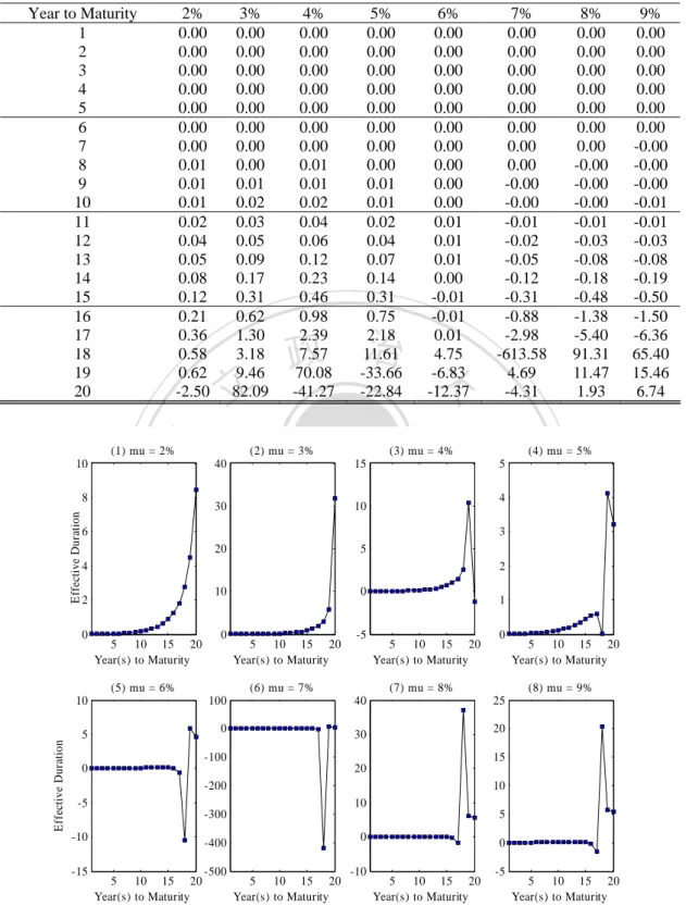
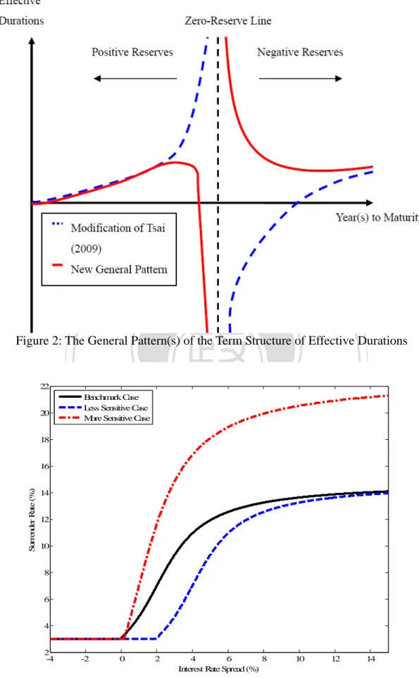
(6) Part One: Characteristics of the Effective Durations and Effective Convexities of Life Insurance Reserves. INTRODUCTION Life insurance reserves are significantly exposed to interest rate risk because the policies usually last for long time and have minimal crediting rates. The high leverage ratios of life insurers aggravate the impact of interest rate variations on solvency. Life insurers therefore should manage the interest rate risk associated with policy reserves in a prudent way, and this starts with measuring the risk correctly. One way to evaluate the interest rate risk of a life insurer’s policy reserves is to calculate the effective duration. Unlike Macaulay duration and the modified duration,1 the effective duration considers the interest sensitivity of cash flows as well as the term structure of interest rates. The dynamics of interest rates being complex stochastic process are well documented in the literatures (e.g., Chan et al., 1992; Chen, 1996; Dahlquist, 1996; Norman, 1997; Ahlgrim, D’Arcy and Gorvett, 1999). Tsai, Kuo, and Chen ( 2002) and Kuo, Tsai, and Chen (2003) further showed that interest rates are a significant determining factor of surrender rates and the cash flows of life insurance policies are sensitive to interest rates as a result. Using Macaulay duration or the modified duration rather than the effective duration would thus result in erroneous measurement on the interest rate risk of policy reserves (Li and Panjer, 1994; Babble, 1995; Santomero and Babbel, 1997; Briys and Varenne, 1997; 2001).. 立. 政治大. ‧. ‧ 國. 學. y. Nat. sit. n. al. er. io. Tsai (2009) recently identified a term structure of the effective durations of policy reserves. Using a cointegrated vector auto-regression (VAR) model for the relation between the surrender rate and the interest rate, he calculated the effective durations of reserves for policies with different maturities. The calculations brought out some negative and/or extreme values. He then plotted the duration values against the policy maturities and identified a term structure consisting of a pair of curves separated by the so-called zero-reserve line. One curve is in the positive domain and the duration increases with the maturity to infinity; the other is in the negative domain and the duration increases from negative infinity with the maturity. The rationale behind such a term structure is that policy reserves are an increasing function of policy year but start from negative values for non-single-premium policies that have positive net present values (NPVs) to life insurers. The effective durations will be negative when policy reserves are negative and be huge when policy reserves are close to zero.. Ch. engchi. i Un. v. The findings of Tsai (2009), albeit insightful and reasonable, may not be general. The VAR model specifies the one-year interest rate as an AR(2) (auto-regression of order two) process with little mean reversion. It also specifies a particular interest sensitivity of surrender rates. The difference between the policy 1. Macaulay duration and the modified duration assume that the yield curve is flat, the curve moves in a parallel fashion, and the cash flows of assets or liabilities are independent of interest rates (discount factors). Unless specified, the durations in this paper are effective durations. 5.

(7) crediting rate and the long-run mean of interest rates assumed in the interest rate model is, apparently, a determining factor to policy reserves and thus the effective durations. So is the interest sensitivity of surrender rates. Tsai (2009) however was not able to conduct the sensitivity analysis on the parameters of the interest rate model and robustness tests across alternative interest rate – surrender rate relations due to the use of an empirical VAR model. In this paper we choose common and flexible interest rate and surrender rate models to scrutinize the generality of the findings in Tsai (2009). We employ the Cox, Ingersoll, and Ross (1985; CIR) model as the interest rate model and follow Babbel et al. (2002) and Kim (2005) in using arctangent functions to model how the surrender rate reacts to the spreads between market interest rates and the policy crediting rate.2 The use of the CIR model enables us to investigate how the long-run mean, volatility, and mean reversion of interest rates may affect the term structure of reserve durations.3 Employing the arctangent function grants us the flexibility in assigning the sensitivity of surrender rates to the spreads and allows us to investigate the impact of thw sensitivity on the reserve duration.. 政治大. Another contribution of this paper to the literature is analyzing the effective convexities of policy reserves. The importance of convexity in managing the interest rate risk is well known in the finance literature (see Choudhry (2005) and the references therein). In the insurance literature, Babbel and Stricker (1987) were the first to point out how the mismatch of asset convexity and liability convexity could adversely affect a life insurer’s surplus. Santomero and Babbel (1997) reported the effective convexities of the reserves for some products. They however disclosed only the final results without the policy specification, interest rate model, surrender behavior, or any other assumptions. The only paper documenting the calculation of the effective convexities for insurance products was Ahlgrim, D’Arcy, and Gorvett (2004), but that was about the property-casualty insurance. The characteristics of the effective convexities of life insurance reserves, despite of their importance in risk management, remain obscure in the present literature.. 立. ‧. ‧ 國. 學. er. io. sit. y. Nat. al. n. iv n C We find that the results of Tsai about reserve U durations are not general. h (2009) g c hthei long-run His results are valid only for the caseseinnwhich mean of interest rates is. lower than or equal to the policy crediting rate. When the long-run mean is higher than the policy crediting rate, the term structure of the effective durations may exhibit a different pattern to the one in Tsai (2009). A reverse pattern would even emerge when surrenders are sensitive to the spread and the long-run mean is higher than the policy crediting rate. Contrary to Tsai (2009), we find that the effective duration can be positive even for the policies with negative reserves (i.e., positive NPVs) and can be negative for positive reserves. The rationale behind our findings is that the interest-sensitive surrender behaviors coupled with persisting positive spreads will make policy reserves become increasing functions of interest rate shocks. Tsai’s results are therefore more suitable under the expectation of no 2. Kim (2005) stated that insurers often fitted surrender rates with an arctangent function of the spreads. Doll et al. (1998) also argued for the arctangent function to depict the interest sensitivities of surrender behaviors. 3 We also tried other popular interest rate models such as Vasicek and Hull-White models. Our findings are robust across these models. 6.

(8) significant and persisting interest rate rises, and our findings are more applicable when insurers expect significant long-run rises of interest rates. Our findings are particularly relevant to the conventional savings-oriented products including annuities and endowment that have low policy crediting rates and interest-sensitive surrender rates. The results of this paper have significant implications to the asset-liability management of life insurers, especially to the insurers that issued policies with low policy crediting rates during the past low-interest-rate era. With regard to convexity, we find that the effective convexities of life insurance reserves may be negative. The effective convexities and effective durations may have opposite signs, and the effective convexities are more volatile than the effective durations. Furthermore, we cannot identify any general pattern for the term structure of effective convexities. The effective convexities exhibit irregular patterns because the relation between the initial short rate and reserves changes with policy maturity considerably. The changes in the relation originate from the interest sensitivity of surrender rates. The relation is also affected by long-run mean level of interest rates. Life insurers should pay attention to the irregularities of effective convexities for accurate asset-liability management and the management should be conducted dynamically as a result.. 立. 政治大. ‧. ‧ 國. 學. The remainder of this article is organized as follows. Section 2 describes the specifications of the analyzed policies. It also explains how we measure the interest risk of policy reserves by calculating the effective durations and effective convexities. Section 3 describes the term structure model of interest rates and the arctangent function used to model the relation between the surrender rate and the spread between the market interest rate and policy crediting rate. It also specifies the model parameters. Section 4 and Section 5 present the results about the effective durations and effective convexities, respectively. Section 6 summaries our findings and concludes the paper.. er. io. sit. y. Nat. al. v. n. POLICY SPECIFICATIONS AND MEASURES OF THE INTEREST RATE RISK. Ch. engchi. i Un. Cash Flows of a Twenty-Year Endowment Policy. We analyze the same twenty-year endowment policies as in Tsai (2009) to facilitate comparisons between his and our results. The policies were issued to 30-year-old males in different years. Death benefits and surrender values are assumed to be paid at the end of the year while premiums and expenses are received and paid at the beginning of the year. The expected net cash flow at time t ( t ∈ N ) for the policy that is at the beginning of policy year k (i.e., sold k-1 years ago; 1 ≤ k < 20 and 1 ≤ t < 20 − k + 1 ) but after the k-th net premium being collected can then be represented as:4. 4. Note that the insured is at age 30+k-1 when the policy is at the beginning of policy year k. 7.

(9) E ( NCFt | k ) = d s (τ ) (d ) (τ ) (s) [( t −1 p30 + k −1 × q30+ k −1+ t −1 × B ) + ( t −1 p30+ k −1 × qt × Bk −1+ t ) ]. (1). cm vcost (τ ) - t p30 ) − λk −1+t ], + k −1 × [π × (1 − Lk −1+ t − L. where. t. (τ ) p30 + k −1 is the probability that the policy for an insured with the age of. (d ) 30 + k − 1 remains valid for t years,5 q30 + k −1+ t −1 is the probability of the insured with. the age of 30 + k − 1 + t − 1 dying within one year, B d denotes the death benefit paid at the end of the year in which the insured dies, qt( s ) is the probability that the policy is surrendered in year t ,6 Bks−1+t denotes the cash surrender value paid at the end of policy year k − 1 + t ,7 π denotes the level premium received at the beginning of each surviving year, Lcm k −1+t represents the commission rate for the commissions paid at the beginning of policy year k − 1 + t , Lvcost stands for the variable cost rate, and λk −1+t represents the fixed cost paid at the beginning of policy year k − 1 + t .8. 政治大. At the policy due date (i.e., t = 20 − k + 1 and 1 ≤ k ≤ 20 ), no premiums are paid by the insured. We further assume that neither commissions nor variable and fixed costs are incurred at maturity. Thus, the second term of Equation (1) vanishes and is replaced by the term denoting the expected surviving benefit: (τ ) (d ) d E ( NCF20−k +1 | k ) = ( 20−k p30 + k −1 × q49 × B ) (2) s suvr (τ ) (s) (τ ) + ( 20−k p30 . + k −1 × q20− k +1 × B20 ) + 20− k p30+ k −1 × B. 立. ‧. ‧ 國. 學. The actuarial assumptions about some of the above variables are shown in Table A1.. er. io. sit. y. Nat. Policy Reserves. The present value of the expected net cash flows associated with the policy right after the k-th net premium is received, Rk , can then be expressed as:. n. al. Ch. Rk = ∑ t =1. 20 − k +1. engchi. i Un. [ E ( NCFt | k ) × vt ] ,. v. (3). where vt denotes the discount factor for the expected net cash flow at time t . Rk represents the present value of the expected liability associated with the policy that just collected the k-th net premiums, given an interest rate path and the corresponding surrender rate path.9 Since interest rates are random and cause surrender rates to be random as well, we follow the framework of Wilmott (1998) to simulate the random Note that 0 p30(τ +) k −1 =1. The upper script (τ) indicate a function referring to all causes or total force of decrement. Two causes of decrement, death and surrender, are considered in this paper and are denoted by the upper scripts (d) and (s) respectively. 6 Note that 1 - q30( d +) k −1+ t −1 - qt( s ) = 1 p30(τ +) k −1+ t −1 . A policy not terminated in a year by death or surrender means that the policy remains valid for a year. Furthermore, (τ ) (τ ) (τ ) , i.e., the probability of a policy with an insured age 30+k-1 being valid t −1 p30 + k −1 × 1 p 30 + k −1 + t −1 = t p30 + k −1 for t years equals the probability of the policy being valid for t-1 years times the probability of the policy with the insured age 30+k-1+t-1 remaining valid for one more year. 7 This is equivalent to saying that the cash surrender value is paid at the end of year t. 8 The time line regarding the above cash flows is plotted in Figure A1 for further clarification. 9 The expectation is taken over the probabilities of decrement. 5. 8.

(10) variable Rk . Measures of Interest Rate Sensitivity We follow Fabozzi (1998) and Hayre and Chang (1997) in calculating the effective duration (ED) and effective convexity (EC) of a financial product. The ED and EC of the policy reserve are thus defined as follows: 10 E ( Rk r0 − ∆r0 ) − E ( Rk r0 + ∆r0 ) , and (4) ED = 2∆r0 ⋅ E ( Rk r0 ) EC =. E ( Rk r0 − ∆r0 ) + E ( Rk r0 + ∆r0 ) − 2 × E ( Rk r0 ) (2∆r0 ) 2 × E ( Rk r0 ) ⋅. ,. (5). where r0 denotes the initial short rate of interest and ∆r0 denotes the change of the initial short rate which is specified as 25 basis points in later calculations. SURRENDER RATE AND INTEREST RATE MODELS Interest Rate Model. 立. 政治大. ‧. ‧ 國. 學. We choose the famous CIR model to simulate interest rates. The CIR model is a mean-reverting process in which the volatility of the short rate is proportional to the square root of the short rate. The discrete-time version of the model is: rs +∆s − rs = κ ⋅ [ µ − rs ]∆s + σ s rs Z s ∆s , (6). n. al. er. io. sit. y. Nat. where rs is the short rate at time s (s ≥ 0), κ reflects the speed of the mean reversion, µ represents the long-term mean to which rs tends to revert to over time, ∆s denotes the time interval, σ s indicates the volatility of rs , and Z s denotes a random number generated from the standard normal distribution.. i Un. v. Although the continuous-time version of the CIR model guarantees positive short rate, the discrete-time version may generate some negative values due to discretization errors. We resort to Euler discretization (Glasserman, 2003) for the exact transition of the short rate so that our simulated rs +∆s are all positive. More specifically, if rs +∆s follows the CIR process, then rs +∆s is distributed as. Ch. engchi. σ s 2 {1 − exp(−κ∆s)}/ 4κ times a non-central chi-square random variable with degrees of freedom d = 4µκ / σ s 2 and a non-centrality parameter λ = [4κ exp( −κ∆s ) / σ s 2 {1 − exp( −κ∆s )}]rs . This transition allows us to simulate the values of rs directly from their exact distribution and maintain one the of major appealing feature of the CIR model. We adopt the parameter values and simulation set up used in Ahlgrim et al. (2004) to simulate paths of annual interest rates and discount factors. They set. 10. The expectation here is taken over random interest rates and surrender rates. E ( Rk | r0 ) can be regarded as the policy reserve marked to the market using the current term structure. 9.

(11) κ = 0.25 , σ s = 0.08 , and the time interval as a quarter.11 To see how the long-term mean of interest rates may affect policy reserves and the effective durations, we experiment with different values of µ within the range of 2% to 9%.12 The initial short rate is assumed to be the same as the policy crediting rate, 4%.13 Since cash flows are incurred annually, we follow Ahlgrim et al. (2004) to compound the quarterly rates into annual rates of interest, denoted as rta. The discount factor is then calculated as: vt = [(1 + r1a )(1 + r2a )L(1 + rt a )]−1 . Surrender Rate Model For a policy with saving property, Doll et al. (1995), Babbel et al. (2002) and Kim (2005) proposed to model the surrender rate as an arctangent function of the spread between a market interest rate and the policy crediting rate.14 They argued that two characteristics of surrender behaviors should be captured by the model.15 Firstly, policyholders have higher incentives to surrender their policies when the spread gets larger. Secondly, the surrender rate should have a lower bound and an upper bound as implied by the historical data. For instance, Tsai, Kuo, and Chen (2002) and Kuo, Tsai, and Chen (2003) observed the possible existence of a “natural” surrender rate similar to the existence of the natural unemployment rate. They also observed that the surrender rate in the US never exceed 21.1%. We therefore model the surrender rate as a monotonically increasing function of the spread with a lower bound as the following arctangent function:16 qt( s ) = max{lb, p1 + p2 × tan −1 ( p3 ⋅ ( rt a − rp ) − p4 )} , (7). 立. 政治大. ‧. ‧ 國. 學. where qt( s ) denotes surrender rate at time t, p1, p2, p3, and p4 are model parameters,. sit. y. Nat. and rp is the policy crediting rate.17. n. al. er. io. As a benchmark, the parameters (p1, p2, p3, p4) are set as (0.07, 0.05, 50, 1) with the lower bound of 3%. The arctangent function specified by these parameters has the saddle point at rt − rp = 2% , qt( s ) = 7% , and the resulted probability of. Ch. i Un. v. receiving surviving benefits is about 17% when µ is set at 6%. The parameters are chosen so that the probability of receiving surviving benefits is close to that implied by the historical surrender rates from 1969 to 1988 (American Council of Life. engchi. 11. Their values are indeed taken from Chen et al. (1992). We also experimented with different values of κ and σ s but found that they do not affect the findings about the characteristics of the term structures of ED and EC. 13 We also tried other values for the initial short rate. The impacts of such changes are immaterial in almost all cases and leave the term structures of ED and EC intact. 14 Be compared with the econometric model, complementary log-log model, in Kim (2005), surrender rates are also fit in with an arctangent model soundly. 15 Doll et al. also proposed that surrender should be tempered by a surrender charge. We regard the surrender charge as nil to simplify the arctangent function. Also, the results of effective duration and effective convexities are indifferent from the presence of a surrender charge. 16 Although we do not have an explicit upper bound in the formula, the surrender rate is capped as Figure 3 will show later. 17 By the first-order and second-order differentiation of qt( s ) at rt a − rp on the differentiable interval, 12. we get the saddle point of the arctangent surrender function which is at rt − rp = p4 / p3 , qt( s ) = p1 . the saddle point, the marginal surrender rate is p2 p3 . 10. At.

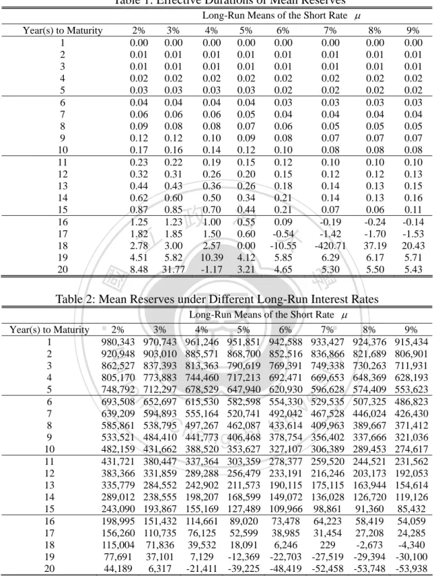
(12) Insurers, 1999) and the 1980 CSO male mortality table.18 TERM STRUCTURE OF EFFECTIVE DURATION The effective durations of mean reserves calculated under different levels of µ are reported in Table 1.19 We see that some EDs are negative, and this is consistent with Tsai (2009). He argued that EDs are negative because the corresponding mean reserves are negative. Policies with negative mean reserves are indeed assets to the insurance company, and designating these “assets” as liabilities on the balance sheet results in these “negative liabilities” having negative durations. The property that mean reserves decrease with a rise/shock in the interest rate holds whether these policies with negative mean reserves are treated as assets or liabilities. [Insert Table 1 Here] We however found counter examples to the above Tsai’s argument. The effective durations can be positive while the corresponding mean reserves are negative, and positive mean reserves may have negative EDs. The mean reserves corresponding to the EDs in Table 1 are shown in Table 2. We can see that the mean reserves maturing twenty years later are -$39,225, -$48,419, and -$52,458 when µ = 5%, 6%, and 7% respectively. This sold policy is an asset to the insurer because the long-run mean of the short rate is higher than the policy crediting rate. Its mean reserves however have positive EDs of 3.21, 4.65, and 5.30. On the other hand, the mean reserves maturing eighteen years later are $6,246 and $229 when µ = 6% and 7%, but their EDs are -10.55 and -420.71. Similar cases can be found for the reserves maturing seventeen years later when µ = 7% and 8%.. 立. 政治大. y. ‧. ‧ 國. 學. Nat. er. io. sit. [Insert Table 2 Here]. When we plot the results of Table 1 as in Figure 1, we spot the patterns opposite to that of Tsai (2009). In the cases of µ = 6%, 7%, and 8%, the EDs increase from zero first but then decrease until becoming negative as the policy’s maturity increases from one year to eighteen or nineteen years. The EDs jump to the positive domain for longer maturities and then start decreasing. We speculate the general pattern of the term structure of the EDs for these cases are as the red curves in Figure 2.. n. al. Ch. engchi. i Un. v. [Insert Figure 1 and Figure 2 Here] 18. This twenty-year period is chosen to be within the sampling period used in estimating the parameters of the interest rate model. 19 The values of many EDs in Table 1 are rather small mainly due to the mean-reverting property of the CIR model. A shock to the initial interest rate fades away as (simulation) time goes by and leaves mid-run and long-run interest rate levels almost intact. Mean reserves hence do not change much and have small EDs. Experimenting with alternative mean-reverting speeds, we confirmed that the values of most EDs decreased with the speeds. The interest sensitivity of surrenders also contributes to the small values of the EDs. When we remove the mean-reverting property of the interest rate model as well as the interest sensitivity of surrenders and calculate the modified durations, the values become close the years to maturity. For instance, the modified durations of the policy reserves maturing 1 year and 5 years later are 0.96 and 4.86 respectively when the interest rate and surrender rate are set at 4%. 11.

(13) The three key conditions resulting in the above pattern are: the long-run mean of interest rates being higher than the policy crediting rate, the surrender rate being sensitive to the spread between the market interest rate and policy crediting rate, and the policy being issued few years ago with small mean reserves. When the first two conditions emerge, a positive interest rate shock will induce more policyholders to surrender their policies. Furthermore, the pre-determined cash values paid to these policyholders are larger than the “fair” mean reserves since the cash values are determined under the assumption that µ = 4% while the mean reserves are marked-to-market by a higher µ . These surrenders therefore will increase the reserves. Since these policies have small mean reserves (the third condition), the impact of these surrenders may outweigh the effect of the present value decreasing with the increased initial short rate and thus cause mean reserves to increase. We illustrate the above reasoning using some examples. At µ = 6%, the mean reserves maturating twenty, nineteen, and eighteen years later are -$48,419, -$22,703, and $6,246 respectively as shown in Table 2. The corresponding surrender values are $0, $8,160.77, and $39,789.39 from Table A1. A 0.25% interest rate shock will increase the surrender probability and causes the mean reserves to increase by $641, $508, and $393 respectively if we hold rt a unchanged. On the other hand, a 0.25% interest rate shock will cause the present values of the mean reserves to decline by $70, $174, and $228 when we assume that the surrender probability does not increase. The net changes are $571, $334, and $165 and thus results in the effective durations of 4.72, 5.88, and -10.55 in Table 1, respectively.20. 立. 政治大. ‧. ‧ 國. 學. n. al. er. io. sit. y. Nat. Our findings and the above reasoning demonstrate the importance of the long-run mean of interest rates, the interest sensitivity of the surrender rate, and the policy’s time to maturity in determining the effective durations of mean reserves.21 Comparing the EDs across the columns in Table 1 and/or examining the graphs in Figure 1, we see clearly the importance of µ in determining the EDs. This implies that life insurers should pay special attention to their estimates on the long-run interest rate level when implementing asset-liability management strategies. The importance of the long-run mean is obscure in Tsai (2009).22. Ch. engchi. i Un. v. The importance of the interest-sensitive surrender rate in determining the effective durations of mean reserves was not explored in Tsai (2009) either. We illustrate the importance by setting alternative parameter sets of the arctangent function and examining the resulting term structures of the EDs. The parameters (p1, p2, p3, p4) are set as (0.1, 0.05, 50, 0.5) to indicate the more sensitive behavior and are chosen to be (0.05, 0.05, 50, 2) to represent the less sensitive surrender behavior.23 20. The duration figures are slightly different from those in Table 2 because we use only the positive interest rate shock to calculate EDs here but Table 2 employs Equation (4) that takes into account of both positive and negative shocks. 21 The importance of time to maturity in determining Macaulay and modified durations is well known and self-evident. Tsai (2009) documented its importance in determining the effective durations of mean reserves. We confirm this importance again in this paper but decide not to elaborate it further for the sake of paper length. 22 An interesting characteristic of the VAR model in Tsai (2009) is that changes in the initial interest rate cause similar changes in the mean of the simulated interest rates. Their effects on the EDs therefore mingle together and are difficult to distinguish from each other. 23 The lower bound of the surrender rate is kept as 3% for these two types of surrender behaviors. 12.

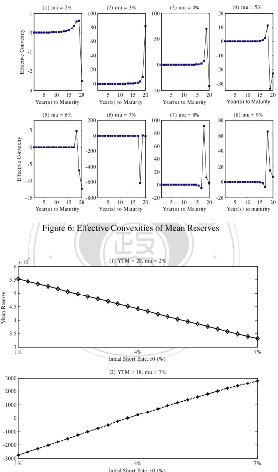
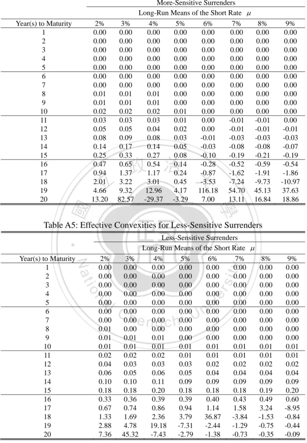
(14) The arctangent functions associated with these two parameter sets along with the benchmark set are plotted in Figure 3, and the resultant term structures of the EDs are shown in Figure 4 and Figure 5.24 [Insert Figures 3, 4, and 5 Here] The patterns of the term structures in Figure 4 are consistent with Figure 1 and conform to the general pattern depicted by the red curves in Figure 2. Figure 5 contains patterns similar to those in Tsai (2009) with a distinction: some recently issued policies have negative mean reserves but positive effective durations. This phenomenon emerges when the long-run mean µ is significantly larger than the policy crediting rate (e.g., µ = 8% or 9%). The large spread induce the surrenders that have cash values much larger than the “fair” policy values and cause mean reserves to increase, even when the surrender rate is sensitive to the spread with a minor degree only. We plot this modified pattern of Tsai (2009) as the blue curves in Figure 2. The above findings and reasoning are robust across values of κ and σ r . We experimented with κ = 0.1, κ = 0.18, and σ s = 0.03. All stories remain intact. We thus can conclude that the pattern identified in Tsai (2009) represent the cases in which the long-run mean of interest rates is not above the policy crediting rate to a certain extent. If the long-run mean is significantly higher than the policy crediting rate, his pattern has to be modified (as the blue curves in Figure 2) even when the surrender rate exhibits low sensitivity to the spread. Higher sensitivities of surrender rates will result in a pattern opposite to the pattern of Tsai (2009) as the red curves in Figure 2 when the long-run means of interest rates are higher than the policy crediting rate. The newly found pattern reflected by some graphs of Figure 1 and Figure 5 results from high sensitivity of surrender rates (and the long-run means of interest rates being higher than the policy crediting rate). In short, the interest sensitivity of the surrender rate and the long-run interest rate level are critical in determining the term structure of the effective durations.. 立. 政治大. ‧. ‧ 國. 學. n. er. io. sit. y. Nat. al. Ch. i Un. TERM STRUCTURE OF EFFECTIVE CONVEXITY. engchi. v. In addition to identifying new term structure patterns of reserve durations, we further calculating the effective convexities of mean reserves for policies maturing in different years. The results are reported in Table 3 and plotted in Figure 6. They are new to the literature. [Insert Table 3 and Figure 6 Here] In Table 3 and Figure 6, we find three features of effective convexities. Firstly, many ECs are negative that were not seen in the insurance literatures. Secondly, the sign of ECs may not be the same as that of EDs. It may not be the same as that of mean reserves either. Thirdly, the term structure of ECs does not exhibit a general pattern and thus does not have the same pattern as that of EDs. The negative ECs emerge when mean reserves are concave functions of initial short rate. For different years to maturity, the mean reserves function of initial short 24. The corresponding values of these EDs are displayed in Table A2 and Table A3. 13.

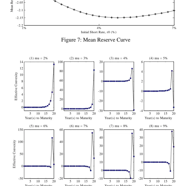
(15) rate might be concave upward/downward or even U-shaped. For example, at µ = 2%, the mean reserves function maturing twenty years is concave downward in the positive range. Then we have a negative EC (-2.50) accompanied with a positive ED (8.48). At µ = 7%, the mean reserves function maturing eighteen years is concave downward from negative to positive range. At this case, we have a negative EC (-613.58) as well as a negative ED (-420.71). At µ = 4%, the mean reserves function maturing twenty years is U-shaped with negative range. At this case, we derive a negative EC (-41.27) as well as a negative ED (-1.17). The mean reserves function in the above three cases are shown in Figure 7. [Insert Figures 7 Here] Comparing Table 1 and 3, we find the sign of EDs and ECs are not consistent. For example, at µ = 5%, we have negative ECs (-33.66 and -22.84) accompanied with positive EDs (4.12 and 3.21) when policy maturing nineteen and twenty years. At µ = 6%, we have positive ECs (4.75) accompanied with negative EDs (-10.55) when policy maturing eighteen years. At µ = 7%, 8% and 9%, we have more examples that negative ECs are accompanied with positive EDs when policy maturing from seven and fifteen years. The inconsistency of the sign of ECs and EDs results from interest-sensitive surrenders and long-run mean of interest rates. Both factors lead the mean reserves function being increasing/decreasing or even not monotonic with initial short rate. Then sign of EDs and of ECs are not consistent.. 立. 政治大. ‧ 國. 學. ‧. The negative ECs are new to insurance literatures but not to finance literatures. Corporate bonds with callable option are accompanied with negative ECs. Douglas (1990) founded that the callable bonds have both positive and negative ECs. The call features, expected trend in interest rates, and market yield volatility would determine whether the EC is positive or negative. Douglas’ conclusions can be evidences for our explanations of negative ECs of mean reserves of endowment policies. Meanwhile, the surrender feature of endowment and the long-run mean of interest rates determine the positive or negative ECs of mean reserves of policy.. n. er. io. sit. y. Nat. al. Ch. engchi. i Un. v. We are not able to spot a general pattern of ECs across different long-run mean of interest rates and years to maturity. In the cases of µ = 2% to 5%, the ECs increase from zero for early maturities and increase from negative range when mean reserves turn to be negative. In the cases of µ = 6%, the ECs increase from zero for early maturities but jump to negative range. Meanwhile, when mean reserves turn to be negative, the ECs become decreasing. In the cases of µ = 7% to 9%, the ECs decrease from zero to negative range for early maturities. When mean reserves turn to be negative, the ECs of mean reserves then decrease from positive range. Under these cases, the term structure of ECs exhibits an irregularity. Thus, due to the negative ECs and the inconsistency of the sign of ECs and EDs, we are unable to generalize the term structure of ECs across different long-run mean of interest rates and years to maturity. The irregularities of the term structures of ECs originate from the interest sensitivity of surrender rates as well as the long-run mean of interest rates and the former dominates the irregularities. In the case of more-sensitive surrenders, the irregularity of term structures of ECs become more severe. The term structures of 14.

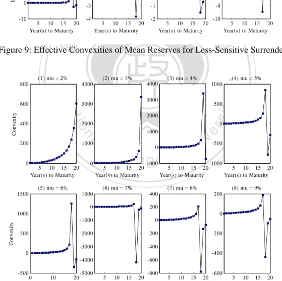
(16) ECs for more-sensitive surrenders are shown in Figure 8. Higher sensitivities of surrender rates will result in an irregular pattern. In the case of less-sensitive surrenders, the term structures of ECs turn to be regular and are similar to the term structures of convexities of mean reserves. The term structures of ECs for less-sensitive surrenders are shown in Figure 9 and the term structures of convexities of mean reserves are shown in Figure 10.25 Under fixed interest rates and surrender rates, the term structures of convexities are similar to the term structures of modified duration addressed in Tsai (2009). This is because fixed interest rates and no interest-sensitive surrenders lead the mean reserves function to be monotonic and simplified. CONCLUSIONS The policy reserves of life insurance are exposed to significant interest rate risk due to the long-run protection nature of life insurance. The insurance literatures pinpointed the significance of interest-sensitive cash flows in determining the interest rate risk of policy reserves and argued strongly for the usage of effective duration and effective convexity rather than the simpler Macaulay and modified measures. Recently, Tsai (2009) identified a term structure of the effective duration of policy reserves using a specific VAR model of interest rates and surrender rates.. 立. 政治大. ‧. ‧ 國. 學. We extend the literature by two ways. Firstly, we re-examine the term structure pattern identified by Tsai (2009) through utilizing more general and flexible models. The use of the popular CIR model enables us to examine how the characteristics of interest rates such as the long-run mean, mean-reverting speed, and volatility may affect the pattern. Using the arctangent function to model how the surrender rate reacts to the spread between the policy crediting rate and market interest rates renders us the flexibility in specifying the interest sensitivity of the surrender rate. Secondly, we illustrate the term structure of the effective convexity of policy reserves. The importance of convexity in managing fixed-income security investments is well known, and our illustration is new to the insurance literature.. er. io. sit. y. Nat. al. n. iv n C We found that the term structure of reserve durations identified by Tsai h pattern n gwhen c h itheUlong-run mean of short rates is (2009) is not universal. His pattern isevalid. not above the policy crediting rate and/or the surrender rate is not sensitive to the interest spread. The term structure pattern changes radically, as demonstrated in Figure 2, when the long-run mean is higher than the policy crediting rate and the surrender rate exhibits certain degree of sensitivity to the interest spread. Tsai’s result needs to be revised even when the surrender rate is not sensitive to the spread if the long-run mean is significantly higher than the policy crediting rate. The reason why Tsai (2009) did not detect our newly identified patterns is because his VAR model consists of an AR(2) process of the one-year interest rate with little mean reverting and a surrender rate process featuring only moderate interest sensitivity. Such an interest rate model obscures the distinction between a short-term interest rate shock and the change in the long-run mean. Being stuck with the surrender rate model specified by the vector-autoregression structure, Tsai (2009) was 25. The ECs under more-sensitive surrenders and less-sensitive surrenders are listed in Appendix Table 4 and 5. 15.

(17) not able to explore alternative sensitivities of surrender rates to interest rates. findings, therefore, do not represent universal cases.. His. Our findings signify the critical roles played by the long-run mean of interest rates and the interest sensitivity of surrender rates in determining the term structure pattern of reserve durations. They have material implications to the life insurers that sell savings-oriented products with fixed crediting rates that are popular in annuity markets and in Asia life insurance markets during low interest rate eras. These life insurers will suffer severely from the disintermediation happened in high interest periods, if they do not have correct estimates on the effective durations of their products and implement appropriate asset-liability management. The damages may be brought by the awaiting recoveries from the recent economic downturns that accompany interest rate rises. Our findings about the effective convexities of policy reserves have practical implications as well, in addition to the contribution to the literature. We find that the effective convexities of mean reserves might be negative for some years to maturity and term structure of effective convexities can not be generalized. Life insurers hence should pay attention to effective convexities when implementing asset-liability management. The irregular term structure patterns of the effective convexities further call for a dynamic management.. 立. 政治大. ‧. ‧ 國. 學. n. er. io. sit. y. Nat. al. Ch. engchi. 16. i Un. v.

(18) REFERENCES Ahlgrim, K. C., S. P. D’Arcy, and R. W. Gorvett, 1999, Parameterizing Interest Rate Models, Casualty Actuarial Society Forum Summer, 1-50. Ahlgrim, K. C., S. P. D’Arcy, and R. W. Gorvett, 2004, The Effective Duration and Convexity of Liabilities of Property-Liability Insurers under Stochastic Interest Rates, Geneva Papers on Risk and Insurance Theory 29, 75-108. American Council of Life Insurance, 1999, Life Insurance Fact Book (Washington DC: American Council of Life Insurance). Babbel, D. F., 1995, Asset-Liability Matching in the Life Insurance Industry, in: The Financial Dynamics of the Insurance Industry, Edward. I. Altman and Irwin. T. Vanderhoof, eds. (New York: IRWIN Professional Publishing). Babble, D. F., J. Gold and C. B. Merrill, 2002, Fair Value of Liabilities: The Financial Economics Perspective, North American Actuarial Journal 6, 12-27.. 立. 政治大 1987, Asset/Liability Management. Babbel, D. F. and R. Stricker, Insurance Perspectives, Goldman Sachs, 1-26.. for Insurers,. ‧ 國. 學. Bowers, N. L., H. U. Gerber, and J. C. Hickman, D. A. Jones, and C. J. Nesbitt, 1997, Actuarial Mathematics, 2nd ed. (Schaumburg, Illinois: Society of Actuaries).. ‧. Briys, E. and F. de Varenne, 1997, On the Risk of Insurance Liabilities: Debunking Some Common Pitfalls, Journal of Risk and Insurance 64, 673-694.. sit. y. Nat. er. io. Briys, E. and F. de Varenne, 2001, Insurance from Underwriting to Derivatives: Asset Liability Management in Insurance Companies (New York: John Wiley & Sons).. al. n. iv n C Chan, K. C., G. A. Karolyi, F. A. Longstaff, and A. B. h e nofgthe i USanders, 1992, An Empirical ch Comparison of Alternative Models Short-Term Interest Rate, Journal of Finance 47, 1209-1227.. Chen, L., 1996, Stochastic Mean and Stochastic Volatility Three-Factor Model of the Term Structure of Interest Rates and Its Applications in Derivatives Pricing and Risk Management, Financial Markets, Institutions and Instruments 5, 1-18. Choudhry, M., 2005, Fixed-Income Securities and Derivatives Handbook: Analysis and Valuation, (Princeton, New Jersey: Bloomberg Press). Cox, J. C., J. E. Ingersoll, Jr., and S. A. Ross, 1985, A Theory of the Term Structure of Interest Rates, Econometrica 53, 385-408. Dahlquist, M., 1996, On Alternative Interest Rate Processes, Journal of Banking and Finance 20, 1093-1119. Doll, D. C., P. C. Elam, J. E. Hohmann, J. M. Keating, D. S. Kolsrud, K. O. 17.

(19) MacDonald, M. S. McLaughlin, T. J. Merfeld, S. D. Reddy, R. R. Reitano, R. S. Robertson, E. L. Robbins, D. Y. Rogers, and H. W. Siegel, 1998, Fair Valuation of Life Insurance Company Liabilities, in: The Fair Value of Insurance Liabilities, Irwin T. Vanderhoof, and Edward I. Altman eds. (New York: Kluwer Academic Publishers). Douglas, L. G., 1990, Bond Risk Analysis: A Guide to Duration and Convexity. (New York: New York Institute of Finance). Fabozzi, F. J., 1998, Valuation of Fixed Income Securities and Derivatives, 3rd ed. (New Hope, Pennsylvania: Frank J. Fabozzi Associates). Glasserman, P., 2003, Monte Carlo Methods in Financial Engineering. (New York: Springer-Verlag). Hayre, L. and H. Chang, 1997, Effective and Empirical Durations of Mortgage Securities, Journal of Fixed Income 6, 17-33.. 政治大. Kim, C., 2005, Modeling Surrender and Lapse Rates with Economic Variables, North American Actuarial Journal 9, 56-70.. 立. ‧ 國. 學. Kuo, W., C. Tsai, and W. Chen, 2003, An Empirical Study on the Lapse Rate: The Cointegration Approach, Journal of Risk and Insurance 70, 489-508.. ‧. Li, D. X. and H. H. Panjer, 1994, Immunization Measures for Life Contingencies, The 4th AFIR Conference, 375-395.. Nat. y. sit. n. al. er. io. Macaulay, F., 1938, Some Theoretical Problems Suggested by the Movements of Interest Rates, Bond Yields, and Stock Prices in the United States since 1856 (New York: National Bureau of Economic Research).. i Un. v. Norman, K. B., 1997, Gaussian Estimation of Single-Factor Continuous Time Models for the Term Structure of Interest Rates, Journal of Finance 52, 1695-1706.. Ch. engchi. Santomero, A. M. and D. F. Babbel, 1997, Financial Risk Management by Insurers: An analysis of the Process, Journal of Risk and Insurance 64, 231-270. Tsai, C., 2009, The Term Structure of Reserve Durations and the Duration of Aggregate Reserves, Journal of Risk and Insurance 76, 419-441. Tsai, C., W. Kuo, and W. Chen, 2002, Early Surrender and the Distribution of Policy Reserves, Insurance: Mathematics, and Economics 31, 429-445. Wilmott, P., 1998, Derivatives: The Theory and Practice of Financial Engineering. (Chichester: John Wiley and Sons).. 18.

(20) TABLES AND FIGURES Table 1: Effective Durations of Mean Reserves 2% 0.00 0.01 0.01 0.02 0.03 0.04 0.06 0.09 0.12 0.17 0.23 0.32 0.44 0.62 0.87 1.25 1.82 2.78 4.51 8.48. 政治大. 立. ‧ 國. Long-Run Means of the Short Rate µ 4% 5% 6% 7% 8% 0.00 0.00 0.00 0.00 0.00 0.01 0.01 0.01 0.01 0.01 0.01 0.01 0.01 0.01 0.01 0.02 0.02 0.02 0.02 0.02 0.03 0.03 0.02 0.02 0.02 0.04 0.04 0.03 0.03 0.03 0.06 0.05 0.04 0.04 0.04 0.08 0.07 0.06 0.05 0.05 0.10 0.09 0.08 0.07 0.07 0.14 0.12 0.10 0.08 0.08 0.19 0.15 0.12 0.10 0.10 0.26 0.20 0.15 0.12 0.12 0.36 0.26 0.18 0.14 0.13 0.50 0.34 0.21 0.14 0.13 0.70 0.44 0.21 0.07 0.06 1.00 0.55 0.09 -0.19 -0.24 1.50 0.60 -0.54 -1.42 -1.70 2.57 0.00 -10.55 -420.71 37.19 10.39 4.12 5.85 6.29 6.17 -1.17 3.21 4.65 5.30 5.50. 3% 0.00 0.01 0.01 0.02 0.03 0.04 0.06 0.08 0.12 0.16 0.22 0.31 0.43 0.60 0.85 1.23 1.85 3.00 5.82 31.77. 學. Year(s) to Maturity 1 2 3 4 5 6 7 8 9 10 11 12 13 14 15 16 17 18 19 20. 9% 0.00 0.01 0.01 0.02 0.02 0.03 0.04 0.05 0.07 0.08 0.10 0.13 0.15 0.16 0.11 -0.14 -1.53 20.43 5.71 5.43. Table 2: Mean Reserves under Different Long-Run Interest Rates. n. al. Ch. y. sit. er. io. 3% 970,743 903,010 837,393 773,883 712,297 652,697 594,893 538,795 484,410 431,662 380,447 331,859 284,552 238,555 193,867 151,432 110,735 71,836 37,101 6,317. ‧. 2% 980,343 920,948 862,527 805,170 748,792 693,508 639,209 585,861 533,521 482,159 431,721 383,366 335,779 289,012 243,090 198,995 156,260 115,004 77,691 44,189. Nat. Year(s) to Maturity 1 2 3 4 5 6 7 8 9 10 11 12 13 14 15 16 17 18 19 20. Long-Run Means of the Short Rate µ 4% 5% 6% 7% 961,246 951,851 942,588 933,427 885,571 868,700 852,516 836,866 813,363 790,619 769,391 749,338 744,460 717,213 692,471 669,653 678,529 647,940 620,930 596,628 615,530 582,598 554,330 529,535 555,164 520,741 492,042 467,528 497,267 462,087 433,614 409,963 441,773 406,468 378,754 356,402 388,520 353,627 327,107 306,389 337,364 303,359 278,377 259,520 289,288 256,479 233,191 216,246 242,902 211,573 190,115 175,115 198,207 168,599 149,072 136,028 155,169 127,489 109,966 98,861 114,661 89,020 73,478 64,223 76,125 52,599 38,985 31,454 39,532 18,091 6,246 229 7,129 -12,369 -22,703 -27,519 -21,411 -39,225 -48,419 -52,458. engchi. 19. i Un. v. 8% 924,376 821,689 730,263 648,369 574,409 507,325 446,024 389,667 337,666 289,453 244,521 203,173 163,944 126,720 91,360 58,419 27,208 -2,673 -29,394 -53,748. 9% 915,434 806,901 711,931 628,193 553,623 486,823 426,430 371,412 321,036 274,617 231,562 192,053 154,614 119,126 85,432 54,059 24,285 -4,340 -30,100 -53,938.

(21) Table 3: Effective Convexities of Mean Reserves 2% 0.00 0.00 0.00 0.00 0.00 0.00 0.00 0.01 0.01 0.01 0.02 0.04 0.05 0.08 0.12 0.21 0.36 0.58 0.62 -2.50. 3% 0.00 0.00 0.00 0.00 0.00 0.00 0.00 0.00 0.01 0.02 0.03 0.05 0.09 0.17 0.31 0.62 1.30 3.18 9.46 82.09. 立. (1) mu = 2%. 2. 10. 20. 5. y. 2 10. al. 0. (5) mu = 6%. Effective Duration. 0. n. 5 10 15 20 Year(s) to Maturity. 4 3. io. 0. 30. 5 10 15 20 Year(s) to Maturity. Ch. -5. 100. 5. 0. 1. v ni. 5 10 15 20 Year(s) to Maturity. engchi U. (6) mu = 7%. 10. 0. 5 10 15 20 Year(s) to Maturity. (7) mu = 8%. (8) mu = 9%. 40. 25. 30. 20. -100. 15. 0. 20 -200. 10. -5. 10 -300. -10 -15. (4) mu = 5%. 5. sit. 4. (3) mu = 4% 15. 8% 0.00 0.00 0.00 0.00 0.00 0.00 0.00 -0.00 -0.00 -0.00 -0.01 -0.03 -0.08 -0.18 -0.48 -1.38 -5.40 91.31 11.47 1.93. ‧. 6. Nat. Effective Duration. 8. (2) mu = 3% 40. er. 10. 政治大. 學. ‧ 國. Year to Maturity 1 2 3 4 5 6 7 8 9 10 11 12 13 14 15 16 17 18 19 20. Long-Run Means of the Short Rate µ 4% 5% 6% 7% 0.00 0.00 0.00 0.00 0.00 0.00 0.00 0.00 0.00 0.00 0.00 0.00 0.00 0.00 0.00 0.00 0.00 0.00 0.00 0.00 0.00 0.00 0.00 0.00 0.00 0.00 0.00 0.00 0.01 0.00 0.00 0.00 0.01 0.01 0.00 -0.00 0.02 0.01 0.00 -0.00 0.04 0.02 0.01 -0.01 0.06 0.04 0.01 -0.02 0.12 0.07 0.01 -0.05 0.23 0.14 0.00 -0.12 0.46 0.31 -0.01 -0.31 0.98 0.75 -0.01 -0.88 2.39 2.18 0.01 -2.98 7.57 11.61 4.75 -613.58 70.08 -33.66 -6.83 4.69 -41.27 -22.84 -12.37 -4.31. 5 0. -400 5 10 15 20 Year(s) to Maturity. -500. 5 10 15 20 Year(s) to Maturity. -10. 0 5 10 15 20 Year(s) to Maturity. -5. 5 10 15 20 Year(s) to Maturity. Figure 1: Effective Durations of Mean Reserves. 20. 9% 0.00 0.00 0.00 0.00 0.00 0.00 -0.00 -0.00 -0.00 -0.01 -0.01 -0.03 -0.08 -0.19 -0.50 -1.50 -6.36 65.40 15.46 6.74.

(22) 政治大. 立. ‧ 國. 學. Figure 2: The General Pattern(s) of the Term Structure of Effective Durations. ‧. io. 16. Surrender Rate (%). al. y. n. 18. sit. Benchmark Case Less Sensitive Case More Sensitive Case. er. 20. Nat. 22. Ch. 14. engchi. i Un. v. 12 10 8 6 4 2 -4. -2. 0. 2. 4 6 8 Interest Rate Spread (%). 10. 12. 14. Figure 3: Arctangent Functions of Surrender Rate to Interest Rate Spread. 21.

(23) (1) mu = 2%. (2) mu = 3% 30. 10. 25. Effective Duration. 12. 8. (4) mu = 5%. (3) mu = 4% 4. 4. 3. 2. 20 2. 6. 15. 4. 0. 10. 1. 5. 0. 2 0. -2. 0 -2. 5 10 15 20 Year(s) to Maturity. 5 10 15 20 Year(s) to Maturity. (5) mu = 6%. -1. (6) mu = 7%. 50. 5 10 15 20 Year(s) to Maturity. -4. (8) mu = 9%. (7) mu = 8%. 15. 40. 10. 8. 8. 6. 10. Effective Duration. 5 10 15 20 Year(s) to Maturity. 30. 6 4. 20. 5. 4. 0. 政治大. 10 0. 0. 0. 5 10 15 20 Year(s) to Maturity. 立 -5. 5 10 15 20 Year(s) to Maturity. -2. 5 10 15 20 Year(s) to Maturity. -2. 5 10 15 20 Year(s) to Maturity. 學. ‧ 國. -10. 2. 2. Figure 4: Effective Durations of Mean Reserves for More-Sensitive Surrenders. y. sit. 5. 0. er. 10. 0 5 10 15 20 Year(s) to Maturity. Ch. 0. engchi. 5 10 15 20 Year(s) to Maturity. -10. (6) mu = 7%. (5) mu = 6%. i Un. v. 5 10 15 20 Year(s) to Maturity (7) mu = 8%. -5. -10. 6. 10. 5. 4. 8. 0. 2. 6. -5. 40. 0. 4. 20. -2. 2. -4. 0. -6. -2. 80. E ffective Duration. 20. 20. al. (4) mu = 5%. 10. 30. 10. 0 -2. 40. (3) mu = 4% 30. n. 2. io. E ffectiv e Duration. 4. Nat. 6. (2) mu = 3% 50. ‧. (1) mu = 2%. 8. 60. 0 -20. 5 10 15 20 Year(s) to Maturity. -8. 5 10 15 20 Year(s) to Maturity. -4. 5 10 15 20 Year(s) to Maturity (8) mu = 9%. -10 -15 -20 5 10 15 20 Year(s) to Maturity. -25. 5 10 15 20 Year(s) to Maturity. Figure 5: Effective Durations of Mean Reserves for Less-Sensitive Surrenders. 22.

(24) (1) mu = 2%. (2) mu = 3%. Effective Convexity. 1. 100. (4) mu = 5%. (3) mu = 4% 100. 20. 80. 10. 0 50. 60 -1. 0. 40. -10 0. 20. -2. -20. 0 -3. 5 10 15 20 Year(s) to Maturity. -30 5 10 15 20 Year(s) to Maturity. (5) mu = 6%. 5 10 15 20 Year(s) to Maturity. (6) mu = 7%. 5. 10. 15. (7) mu = 8%. (8) mu = 9%. 100. 80. 0. 80. 60. 60. 0. -200. 40 40. -5. -400. 20. 政治大 20. -10. -600. 立. 5 10 15 20 Year(s) to Maturity. -800. 0. 0. 5 10 15 20 Year(s) to Maturity. -20. 5 10 15 20 Year(s) to Maturity. -20. 5 10 15 20 Year(s) to maturity. 學. ‧ 國. -15. Figure 6: Effective Convexities of Mean Reserves. 4 3.5 3 1%. y. sit. al. n. 4.5. io. Mean Reserve. 5. (1) YTM = 20, mu = 2%. Nat. 5.5. 4. er. x 10. ‧. 6. Ch. engchi. 4% Initial Short Rate, r0 (%). i Un. v. 7%. (2) YTM = 18, mu = 7%. 3000. Mean Reserve. 2000 1000 0 -1000 -2000 -3000 1%. 20. Year(s) to Maturity. 200 5 Effective Convexity. -50. 4% Initial Short Rate, r0 (%). 23. 7%.

(25) -1.9. x 10. 4. (3) YTM = 20, mu = 4%. Mean Reserve. -1.95 -2 -2.05 -2.1 -2.15 -2.2 1%. 4% Initial Short Rate, r0 (%). 7%. Figure 7: Mean Reserve Curve. (1) mu = 2%. (2) mu = 3%. 14. 6. 80. 10. 4. 10 60. 8 6. 40. 立. 4. 0. 5 10 15 20 Year(s) to Maturity. 5 10 15 20 Year(s) to Maturity. (5) mu = 6%. -20. -2. -30. -4. 5 10 15 20 Year(s) to Maturity. 5 10 15 20 Year(s) to Maturity. (7) mu = 8%. (8) mu = 9%. 50. 40. 40. 30. 30. 20. 10. al. sit. 20. 10. 0. er. 20. y. 40. io. 0. n. -50. 0. (6) mu = 7%. Nat. 0. -10. 60. 100. 50. 2. ‧. 150. 0. 學. 0. 政治大. 20. 2. ‧ 國. Effective Convexity. (4) mu = 5%. 20. 12. Effective Convexity. (3) mu = 4%. 100. 5 10 15 20 Year(s) to Maturity. -20. 0. Ch. engchi. 5 10 15 20 Year(s) to Maturity. -10. i Un. v. 5 10 15 20 Year(s) to Maturity. -10 -20. 5 10 15 20 Year(s) to Maturity. Figure 8: Effective Convexities of Mean Reserves for More-Sensitive Surrenders. 24.

(26) Effective Convexity. (1) mu = 2%. (2) mu = 3% 50. 20. 6. 6. 40. 15. 4. 4. 30. 0 -2. 20. 2. 0. -4. -5. -6. 10. 0. 0 5 10 15 20 Year(s) to Maturity. (4) mu = 5%. 2. 10 5. -2. 5 10 15 20 Year(s) to Maturity. (5) mu = 6%. -10. (6) mu = 7%. -8. 5 10 15 20 Year(s) to Maturity. 5 10 15 20 Year(s) to Maturity. (7) mu = 8%. (8) mu = 9%. 40. 2. 4. 2. 30. 1. 3. 0. 0. 2. -2. -1. 1. -4. 20 10 -2 0 -10. -3. 立. -4. 5 10 15 20 Year(s) to Maturity. 政治大 0. -6. -1. -8. -2. 5 10 15 20 Year(s) to Maturity. -10. 5 10 15 20 Year(s) to Maturity. 5 10 15 20 Year(s) to Maturity. 學. ‧ 國. Effective Convexity. (3) mu = 4%. 8. Figure 9: Effective Convexities of Mean Reserves for Less-Sensitive Surrenders. y. sit. 2000. 2000. 0. al. 1000. n. 200. 0. 500. 1000. 5 10 15 20 Year(s) to Maturity. 0. Ch. 0. engchi. 5 10 15 20 Year(s) to Maturity. -1000. (6) mu = 7%. (5) mu = 6% 1500. er. 400. (4) mu = 5%. 1000. 3000. 3000. io. Convexity. (3) mu = 4% 4000. 4000. Nat. 600. ‧. (2) mu = 3%. (1) mu = 2% 800. i Un. v. 5 10 15 20 Year(s) to Maturity. Convexity. -1000. (7) mu = 8%. 1000. 400. 0. 200. -1000. 0. -2000. -200. -3000. -400. -4000. -600. 5 10 15 20 Year(s) to Maturity (8) mu = 9%. 200. 1000. 0. 500. -200. 0. -500. -500. -400. 0 10 20 Year(s) to Maturity. -5000. 5 10 15 20 Year(s) to Maturity. -800. 5 10 15 20 Year(s) to Maturity. -600. Figure 10: Convexities of Mean Reserves. 25. 5 10 15 20 Year(s) to Maturity.

(27) APPENDICES Table A1: Actuarial Assumptions of the Twenty-Year Endowment Policy Insured’s Mortality Rate At the Beginning of Age of age a Policy Year (d ) qa a k 30 0.0009790 1 31 0.0010055 2 32 0.0010481 3 33 0.0011075 4 34 0.0011826 5 35 0.0012712 6 36 0.0013711 7 37 0.0014807 8 38 0.0015989 9 39 0.0017291 10 40 0.0018749 11 41 0.0020407 12 42 0.0022297 13 43 0.0024446 14 44 0.0026795 15 45 0.0029268 16 46 0.0031784 17 47 0.0034268 18 48 0.0036671 19 49 0.0039091 20 50 N/A 20*. Commission Rate. Bks. Lcm k. N/A 8,161 39789 73,767 110,192 149,173 190,831 235,294 282,707 333,223 387,004 437,655 490,342 545,163 602,227 661,664 723,620 788,259 855,760 926,314 1,000,000. 62.40% 27.00% 20.60% 14.00% 13.00% 12.00% 10.00% 10.00% 10.00% 10.00% 7.00% 7.00% 7.00% 7.00% 7.00% 7.00% 7.00% 7.00% 7.00% 7.00% N/A. 政治大. 學. Fixed Expense λk 4,530 1,359 1,359 1,359 1,359 1,359 1,359 1,359 1,359 1,359 1,359 1,359 1,359 1,359 1,359 1,359 1,359 1,359 1,359 1,359 N/A. Variable Cost Rate. Lv cos t 0.001 0.001 0.001 0.001 0.001 0.001 0.001 0.001 0.001 0.001 0.001 0.001 0.001 0.001 0.001 0.001 0.001 0.001 0.001 0.001 N/A. ‧. ‧ 國. 立. Surrender Value. The death benefit and survival benefit is $1,000,000. The policy is issued to a 30 year-old male, and the annual premium expected to pay at the beginning of each surviving year is $45,300 under the policy crediting rate of 4%.. 2.. The notation 20* is used to denote the end of policy year 20.. 3.. The policy surrendered at the beginning of the first policy year has no surrender value. Neither mortality nor expenses apply any more when the policy matures. We denote all these values as N/A.. sit. y. n. al. er. io. 4.. Nat. 1.. Ch. The variable cost is assumed to be 0.1%.. engchi. 26. i Un. v.

(28) Table A2: Effective Durations for Less-Sensitive Surrenders. Year(s) to Maturity 1 2 3 4 5 6 7 8 9 10 11 12 13 14 15 16 17 18 19 20. 2% 0.00 0.01 0.01 0.02 0.03 0.04 0.06 0.09 0.12 0.17 0.23 0.32 0.44 0.61 0.86 1.22 1.76 2.66 4.22 7.63. 立. 3% 0.00 0.01 0.01 0.02 0.03 0.04 0.06 0.09 0.12 0.17 0.23 0.32 0.45 0.63 0.89 1.29 1.96 3.23 6.43 41.35. Less-Sensitive Surrenders Long-Run Means of the Short Rate µ 4% 5% 6% 7% 8% 0.00 0.00 0.00 0.00 0.00 0.01 0.01 0.01 0.01 0.01 0.01 0.01 0.01 0.01 0.01 0.02 0.02 0.02 0.02 0.02 0.03 0.03 0.03 0.03 0.03 0.04 0.04 0.04 0.04 0.04 0.06 0.06 0.06 0.06 0.06 0.08 0.08 0.08 0.08 0.08 0.12 0.11 0.11 0.11 0.11 0.16 0.16 0.16 0.15 0.15 0.23 0.22 0.22 0.21 0.21 0.31 0.31 0.30 0.30 0.30 0.44 0.43 0.43 0.42 0.42 0.62 0.61 0.61 0.61 0.62 0.89 0.90 0.92 0.94 0.97 1.34 1.38 1.47 1.59 1.78 2.15 2.40 2.94 3.95 7.80 4.21 6.69 62.44 -6.04 -2.14 23.40 -8.27 -2.38 -0.97 -0.30 -5.65 -1.62 -0.37 0.21 0.56. 政治大. 9% 0.00 0.01 0.01 0.02 0.03 0.04 0.06 0.08 0.11 0.15 0.21 0.29 0.42 0.63 1.02 2.12 -20.40 -0.97 0.08 0.79. ‧ 國. 學. Table A3: Effective Durations for More-Sensitive Surrenders. n. al. y. sit. er. io. 2% 0.00 0.01 0.01 0.02 0.03 0.04 0.06 0.09 0.12 0.17 0.23 0.32 0.45 0.63 0.90 1.30 1.93 3.00 5.09 10.85. ‧. Nat. Year(s) to Maturity 1 2 3 4 5 6 7 8 9 10 11 12 13 14 15 16 17 18 19 20. More-Sensitive Surrenders Long-Run Means of the Short Rate µ 3% 4% 5% 6% 7% 0.00 0.00 0.00 0.00 0.00 0.01 0.01 0.01 0.01 0.01 0.01 0.01 0.01 0.01 0.01 0.02 0.02 0.02 0.02 0.02 0.03 0.03 0.02 0.02 0.02 0.04 0.04 0.03 0.03 0.03 0.06 0.05 0.05 0.04 0.04 0.08 0.07 0.06 0.06 0.05 0.11 0.09 0.08 0.07 0.07 0.15 0.13 0.11 0.10 0.09 0.20 0.17 0.14 0.12 0.12 0.28 0.23 0.19 0.16 0.15 0.39 0.31 0.25 0.21 0.19 0.55 0.43 0.33 0.27 0.25 0.77 0.59 0.43 0.33 0.30 1.11 0.83 0.55 0.38 0.33 1.66 1.18 0.68 0.34 0.21 2.64 1.79 0.65 -0.36 -0.92 4.97 3.52 -3.62 42.71 14.04 26.71 -0.95 3.89 4.94 5.12. Ch. engchi. 27. i Un. v. 8% 0.00 0.01 0.01 0.02 0.02 0.03 0.04 0.05 0.07 0.09 0.12 0.15 0.20 0.25 0.31 0.35 0.24 -1.04 9.44 4.95. 9% 0.00 0.01 0.01 0.02 0.02 0.03 0.04 0.05 0.07 0.09 0.12 0.16 0.21 0.27 0.34 0.40 0.35 -0.86 6.82 4.63.

(29) Table A4: Effective Convexities for More-Sensitive Surrenders. Year(s) to Maturity 1 2 3 4 5 6 7 8 9 10 11 12 13 14 15 16 17 18 19 20. 2% 0.00 0.00 0.00 0.00 0.00 0.00 0.00 0.01 0.01 0.02 0.03 0.05 0.08 0.14 0.25 0.47 0.94 2.01 4.66 13.20. 立. More-Sensitive Surrenders Long-Run Means of the Short Rate µ 4% 5% 6% 7% 0.00 0.00 0.00 0.00 0.00 0.00 0.00 0.00 0.00 0.00 0.00 0.00 0.00 0.00 0.00 0.00 0.00 0.00 0.00 0.00 0.00 0.00 0.00 0.00 0.00 0.00 0.00 0.00 0.01 0.00 0.00 0.00 0.01 0.00 0.00 0.00 0.02 0.01 0.00 0.00 0.03 0.01 0.00 -0.01 0.04 0.02 0.00 -0.01 0.08 0.03 -0.01 -0.03 0.14 0.05 -0.03 -0.08 0.27 0.08 -0.10 -0.19 0.54 0.14 -0.28 -0.52 1.17 0.24 -0.87 -1.62 3.01 0.45 -3.53 -7.24 12.96 4.17 116.18 54.70 -29.37 -3.29 7.00 13.11. 3% 0.00 0.00 0.00 0.00 0.00 0.00 0.00 0.01 0.01 0.02 0.03 0.05 0.09 0.17 0.33 0.65 1.37 3.22 9.32 82.57. 政治大. 8% 0.00 0.00 0.00 0.00 0.00 0.00 0.00 0.00 0.00 0.00 -0.01 -0.01 -0.03 -0.08 -0.21 -0.59 -1.91 -9.73 45.13 16.84. 9% 0.00 0.00 0.00 0.00 0.00 0.00 0.00 0.00 0.00 0.00 0.00 -0.01 -0.03 -0.07 -0.19 -0.54 -1.86 -10.97 37.63 18.86. ‧ 國. 學. Table A5: Effective Convexities for Less-Sensitive Surrenders. n. al. Ch. sit. 3% 0.00 0.00 0.00 0.00 0.00 0.00 0.00 0.00 0.01 0.01 0.02 0.03 0.05 0.10 0.18 0.36 0.74 1.69 4.78 45.32. er. io. 2% 0.00 0.00 0.00 0.00 0.00 0.00 0.00 0.01 0.01 0.01 0.02 0.04 0.06 0.10 0.18 0.33 0.67 1.33 2.88 7.36. y. ‧. Nat. Year(s) to Maturity 1 2 3 4 5 6 7 8 9 10 11 12 13 14 15 16 17 18 19 20. Less-Sensitive Surrenders Long-Run Means of the Short Rate µ 4% 5% 6% 7% 8% 0.00 0.00 0.00 0.00 0.00 0.00 0.00 0.00 0.00 0.00 0.00 0.00 0.00 0.00 0.00 0.00 0.00 0.00 0.00 0.00 0.00 0.00 0.00 0.00 0.00 0.00 0.00 0.00 0.00 0.00 0.00 0.00 0.00 0.00 0.00 0.00 0.00 0.00 0.00 0.00 0.01 0.00 0.00 0.00 0.00 0.01 0.01 0.01 0.01 0.01 0.02 0.01 0.01 0.01 0.01 0.03 0.03 0.02 0.02 0.02 0.06 0.05 0.04 0.04 0.04 0.11 0.09 0.09 0.09 0.09 0.20 0.18 0.18 0.18 0.19 0.39 0.39 0.40 0.43 0.49 0.86 0.94 1.14 1.58 3.24 2.36 3.79 36.87 -3.84 -1.53 19.18 -7.31 -2.44 -1.29 -0.75 -7.43 -2.79 -1.38 -0.73 -0.35. engchi. 28. i Un. v. 9% 0.00 0.00 0.00 0.00 0.00 0.00 0.00 0.00 0.00 0.01 0.01 0.02 0.04 0.09 0.20 0.60 -8.95 -0.84 -0.44 -0.09.

(30) The time line below describes the relations among policy year k, insured’s age 30+k-1, and the evaluation time t and where the net cash flows are. t. Insured Age. 1. 30. 2. 31. k-1. 32. k. k-1+t. 30+ k -2 30+ k -1 30+ k. Time. -1. 0. 1. t-1. Figure A1: Illustrative Time Line. 立. 政治大. ‧. ‧ 國. 學. io. sit. y. Nat. n. al. Ch. engchi. 29. k+t. 30+ k -1+t-1 30+ k -1+t 30+ k +t. er. Policy Year. i Un. v. t. t+1.

(31) Part Two: A Promising Asset Allocation and Leverage Strategy for a Life Insurer by Simulation Optimization INTRODUCTION Managing investments is important for life insurers to ensure that funds are available to pay claims when they fall due, in the future. However, conflicts of interest between shareholders, regulators and policyholders make investment decisions difficult. Shareholders of insurers urge them to generate higher returns from investments and underwriting but regulators and policyholders ask them to maintain risk at acceptable levels. Life insurers thus have to manage divergent expectations emanating from both assets and liabilities sides. In this study, we re-think the classic asset allocation problem specifically for life insurers. We propose a non-linear simulation model with stochastic variables to derive promising asset allocations and leverage strategies.. 政治大. Extant literature has covered the asset allocation problem quite extensively. In financial literature, there are two categories of methods to address this problem. One is the mean-variance analysis of Markowitz (1952), which suggests the efficient frontier representing the best portfolios in terms of return-risk tradeoff. The mean-variance analysis, however, is prone to two fundamental flaws: the single-period framework, and the inappropriate utility function assumed for the investor (Brennan et al., 1997). The solution to a static portfolio choice problem can be different from the solution to a multi-period dynamic problem (Campbell, 2000). The other method to construct optimal portfolios originated from Merton (1971; 1990). The literature along this line formulates the asset allocation problem as a stochastic optimal control problem; solutions are characterized by Hamilton-Jacobi-Bellman (HJB) partial differential equations (PDE) but it is difficult to get a closed-form solution from a high-dimensional PDE. Also, numerical solutions of PDE can be obtained only in rare cases. Cox and Huang (1989) made conceptual progress by showing that one can apply the Martingale representation theory to reduce the stochastic dynamic programming problem to a static problem in complete markets. However, few closed-form solutions have been available, except for the simplest cases, and complex hedging terms are difficult to evaluate numerically.. 立. ‧. ‧ 國. 學. n. er. io. sit. y. Nat. al. Ch. engchi. i Un. v. We need a powerful tool to integrate the asset allocation problem and leverage strategies for efficient asset and liability management by life insurers. A company-wide simulation model is one such tool (Browne, Carson and Hoyt, 1999; Browne, Carson and Hoyt, 2001; Kaufmann et al., 2001; and Hardy, 1993, 1996).1 It is a “systemic approach” to financial modeling which projects financial results under a variety of possible scenarios, showing how outcomes might be affected by changing business, competitive and economic conditions.” The system starts with two fundamental equations, as follows:. 1. A company-wide simulation system is often named as “Dynamic Financial Analysis” (DFA) system in the non-life insurance industry. What is called DFA in non-life insurance is also known as “Asset Liability Management” (ALM) in life insurance. 30.