以福衛三號及GRACE低軌衛星GPS資料推算時變地球重力場

國 立 交 通 大 學

土 木 工 程 學 系

博 士 論 文

以福衛三號及 GRACE 低軌衛星 GPS 資料推算時變地

球重力場

Temporal Gravity Changes from FORMOSAT-3 and

GRACE GPS Tracking Data

研 究 生 ： 林 廷 融

指導教授 ： 黃 金 維

以福衛三號及 GRACE 低軌衛星 GPS 資料推算時變地

球重力場

Temporal Gravity Changes from FORMOSAT-3 and

GRACE GPS Tracking Data

研 究 生：林廷融 Student : Ting-Jung Lin

指導教授：黃金維 博士 Advisor : Dr. Cheinway Hwang

國 立 交 通 大 學

土 木 工 程 學 系

博 士 論 文

A Dissertation

Submitted to Department of Civil Engineering

College of Engineering

National Chiao Tung University

in partial Fulfillment of the Requirements

for the Degree of

Doctor of Philosophy

in

Civil Engineering

June 2010

Hsinchu, Taiwan, Republic of China

中華民國九十九年六月

以福衛三號及 GRACE 低軌衛星 GPS 追蹤資料推算時

變地球重力場

研究生：林廷融 指導教授：黃金維 博士

國立交通大學土木工程學系

摘 要

本論文內容是結合福衛三號及 GRACE 衛星高-低衛星追蹤資料反衍時變地 球重力場。為了估算時變重力地位係數，吾人已成功發展兩種重力反衍方法:軌 道擾動解析法及殘餘加速度法，此兩種方法分別應用殘餘軌道擾動量(動態軌道 及動力軌道之差值)及殘餘加速度(觀測加速度及參考加速度之差值)兩種不同觀 測量，分別建立與時變重力地位係數之線性關係後進行估算時變重力地位係數。 吾人首先使用 Bernese 5.0 軟體計算福衛三號及 GRACE 衛星公分級動態軌 道。此後，以標準力模式進行計算作用於福衛三號及 GRACE 衛星上之各種擾動 力，此部分使用之主要計算軟體為 NASA Goddard 研發之 GEODYN II 軟體。福 衛三號表面擾動力如大氣阻力、輻射壓及其他微小表面擾動力須以力模式進行求 解，並於每飛行一圈即解算一組適當表面力參數。所解算之原始 5 秒一筆之六顆 福衛三號衛星及 10 秒一筆之兩顆 GRACE 衛星動態及動力軌道重新取樣為一分 鐘一筆之軌道位置資料，及後以數值微分得到加速度資料分別以為重力場反衍之 用。 吾人以 2006 年 8 月一個月福衛三號及 GRACE 動態及動力軌道資料求解時 變重力地位係數，分別使用軌道擾動解析法及殘餘加速度法處理福衛三號單一解

為 7.5 公分及 6.5 公分。福衛三號單一解可解出某些已知的時變重力訊號，但仍 含有雜訊，合併解則可看出某些程度提升了 GRACE 單一解某些區域時變重力訊 號。 此外，吾人處理自 2006 年 9 月至 2007 年 12 月共 16 個月的福衛三號及 GRACE 精密定軌資料進行每月低階時變重力係數求解至 5 階，使用軌道擾動解析法及殘 餘加速度法所得到之大地起伏變化將與 CSR RL04 解進行比較分析，15 階之合 併 GRACE 解也將進行求解。吾人使用軌道擾動解析法及殘餘加速度法所得到之 低階帶諧係數ΔC₂₀,ΔC₃₀及ΔC₄₀之變化與 SLR 及 CSR RL04 解同期觀測比較， 發現四者變化趨勢極為相似，由 SLR、軌道擾動解析法殘餘加速度法、及 CSR RL04 解 算 之 ΔC₂₀ 年 變 率 分 別 為

(

)

10 10 045 94 . 0 ± × − − 、

(

)

10 10 86 . 0 06 . 1 ± × − − 、

(

)

11 10 78 . 0 15 . 0 ± × − 及

(

)

10 10 86 . 0 98 . 1 ± × − − ，CSR RL04、軌道擾動解析法及殘餘加速度 法解算之ΔC₃₀年變率為

(

)

11 10 07 . 6 58 . 1 ± × − − 、

(

)

11 10 09 . 7 13 . 5 ± × − − 及

(

)

11 10 14 . 8 07 . 7 ± × − − ， 40 C Δ 年變率為

(

)

11 10 06 . 3 46 . 3 ± × − 、

(

)

11 10 91 . 2 20 . 0 ± × − − 及

(

)

11 10 01 . 3 33 . 2 ± × − 。

Temporal Gravity Changes from FORMOSAT-3 and

GRACE GPS Tracking Data

Student : Ting-Jung Lin Advisor : Dr. Cheinway Hwang Department of Civil Engineering

National Chiao Tung University

Abstract

This dissertation is aimed at temporal gravity field recovery from the analyses of

the high-low satellite-to-satellite tracking (hl-SST) data from the COSMIC and

GRACE satellite missions. In order to estimate the time-varying geopotential coefficients, two efficient methodologies, the analytical orbital perturbation (AOP) approach and the residual acceleration (ACC) approach, are developed in the research. With the reference orbits removed, orbital perturbations (difference between kinematic and reference orbits) and residual accelerations (difference between observed and reference accelerations) from the residual orbits are linear functions of the time-varying geopotential coefficients. Such linear functions enable convenient establishments of observation equations to estimate geopotential coefficients.

The Bernese 5.0 software is used to compute the cm-level kinematic orbits of COSMIC and GRACE. The NASA Goddard’s GEODYN II software is used to compute the perturbing forces acting on COSMIC and GRACE satellites based on the standard models of orbit dynamics. The accelerations due to the atmospheric drag, solar radiation pressure and other minor surface forces are estimated by some relevant model parameters over one orbital period from COSMIC’s kinematic and reduced dynamic orbits. The 5s kinematic and dynamic orbits from six COSMIC and the 10s

positional data and then converted to acceleration data by numerical differential for gravity recovery.

To validate the theories and computer programs associated with the AOP and ACC approaches, some experimental solutions of time-varying geopotential coefficients are carried out using one-month (August 2006) of COSMIC and GRACE kinematic and dynamic orbits. The average RMS in RTN directions of reduced COSMIC and GRACE (1 minute) between kinematic orbits and dynamic orbits are about 7.5 and 6.5 cm. The COSMIC solutions reveal several well-known temporal gravity signatures, but contain artifacts. The combined COSMIC-GRACE solutions enhance some local features in the GRACE solutions.

The monthly COSMIC and GRACE precise orbit data from September 2006 to December 2007 (16 months) are processed to recover monthly low-degree (up to degree 5) geopotential coefficients by the AOP and ACC approaches. The geoid variations from such low-degree geopotential coefficients are compared with the CSR RL04 solutions. Two combined solutions by the AOP and ACC approaches (up to degree 15) are also carried out. The monthly variations of the zonal geopotential coefficients ΔC₂₀, ΔC₃₀ and ΔC₄₀ from the AOP and ACC solutions (degree 5)

closely resemble the SLR-derived and CSR RL04 solutions. The rates of ΔC₂₀ from

SLR, AOP, ACC, and CSR RL04 are

(

−0.94±045

)

×10−10,

(

−1.06±0.86

)

×10−10,

(

)

11 10 78 . 0 15 .

0 ± × − _and

(

−1.98±0.86

)

×10−10 , respectively. The rates of ΔC₃₀ from CSR RL04, AOP and ACC solutions are

(

−1.58±6.07

)

×10−11,

(

−5.13±7.09

)

×10−11, and

(

)

11 10 14 . 8 07 . 7 ± × −

− , and the rates of ΔC₄₀ are

(

3.46±3.06

)

×10−11 ,

Table of Contents

Abstract (in Chinese) ... i

Abstract ... iii

Table of Contents ... v

List of Tables ... vii

Lists of Figures ... viii

Chapter 1 Introduction ... 1

1.1 Background ... 1

1.2 Research Objectives ... 7

1.3 Outlines of Thesis ... 8

Chapter 2 Methods for gravity field modeling using GPS observations ... 10

2.1 Introduction ... 10

2.2 Theory of analytical orbital perturbation approach ... 11

2.3 Theory of residual acceleration approach ... 20

Chapter 3 Force modeling and precise orbit determination for COSMIC ... 23

3.1 Introduction ... 23

3.2 Orbit dynamics of COSMIC satellite ... 23

3.2.1 Equations of motion and perturbing potential force ... 24

3.2.2 Atmospheric drag and solar radiation effects on COSMIC satellites ... 26

3.3 Kinematic orbit determination using Bernese 5.0 ... 30

3.4 Dynamic orbit determination using GEODYN II software ... 32

4.1 Introduction ... 42

4.2 Kinematic orbits of COSMIC and accuracy assessment ... 42

4.3 Reference dynamic orbits for COSMIC and GRACE ... 46

4.4 Formulae used in gravity recovery ... 48

4.5 Results of gravity recovery ... 51

Chapter 5 Temporal gravity recovery based on satellite accelerations ... 62

5.1 Introduction ... 62

5.2 Processing of COSMIC and GRACE residual accelerations ... 62

5.2.1 Position data screening ... 63

5.2.2 Computation of residual accelerations ... 66

5.3 Validation of the acceleration method ... 69

5.4 Gravity recovery using COSMIC and GRACE GPS data ... 78

Chapter 6 Low-degree gravity change... 88

6.1 Introduction ... 88

6.2 Data of COSMIC and GRACE ... 88

6.3 Time series of monthly gravity solutions ... 93

6.4 Low-degree zonal coefficients ... 107

Chapter 7 Summary, Conclusions, and Recommendations ... 112

7.1 Summary and conclusions ... 112

7.2 Recommendations for future work ... 113

Reference ... 115

Appendix A: Acronyms ... 123

List of Tables

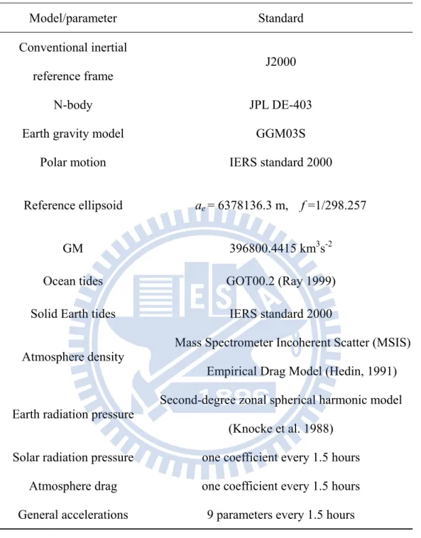
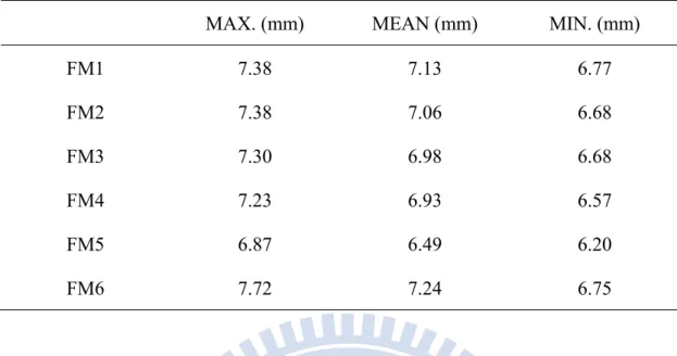
Table 3-1 Standards for the orbit dynamics of COSMIC satellites ... 36 Table 4-1 Statistics of standard errors of normal-point kinematic orbits ... 46

Table 4-2 Different standards for the orbit dynamics of COSMIC and GRACE satellites47

Table 5-1 Average RMS differences between kinematic orbits and dynamic orbits in RTN

directions for six COSMIC and two GRACE satellites (unit: cm) ... 65

Table 5-2 Statistics of percentages of accepted normal-point kinematic orbits (August,

2006) ... 67

Table 5-3 Relative errors of geopotential coefficients from COSMIC-only and

COSMIC-GRACE solutions ... 85

Table 6-1 Numbers of observation files and usable kinematic orbit files from September

2006 to December 2007 ... 90

Table 6-2 Averaged RMS differences between kinematic and dynamic orbits from

List of Figures

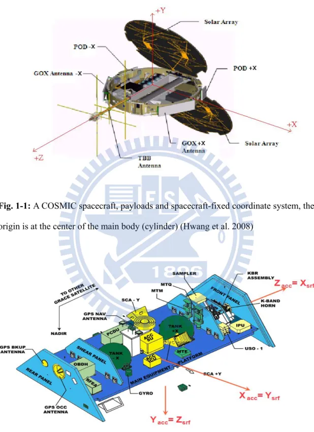
Fig. 1-1 A COSMIC spacecraft, payloads and spacecraft-fixed coordinate system, the

origin is at the center of the main body (cylinder) (Hwang et al. 2008) ... 6

Fig. 1-2 GRACE science instrumentation (http://www-app2.gfz-potsdam.de/pb1

/op/ grace / index_GRACE.html) ... 6

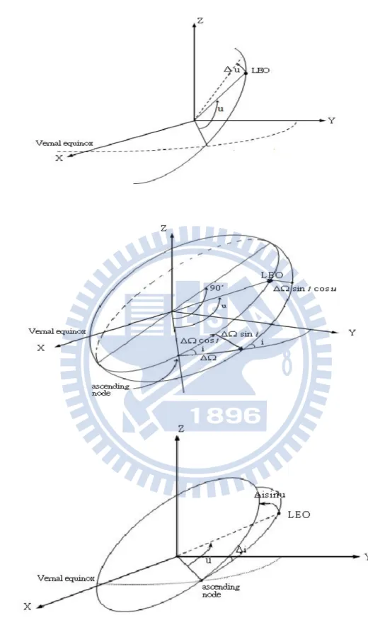
Fig. 2-1 Geometry showing the effects of perturbations in argument of perigee (top), right

ascension of the ascending node and inclination (bottom) on the radial, along-track, and cross-track perturbations at a satellite position (Hwang 2001) ... 12

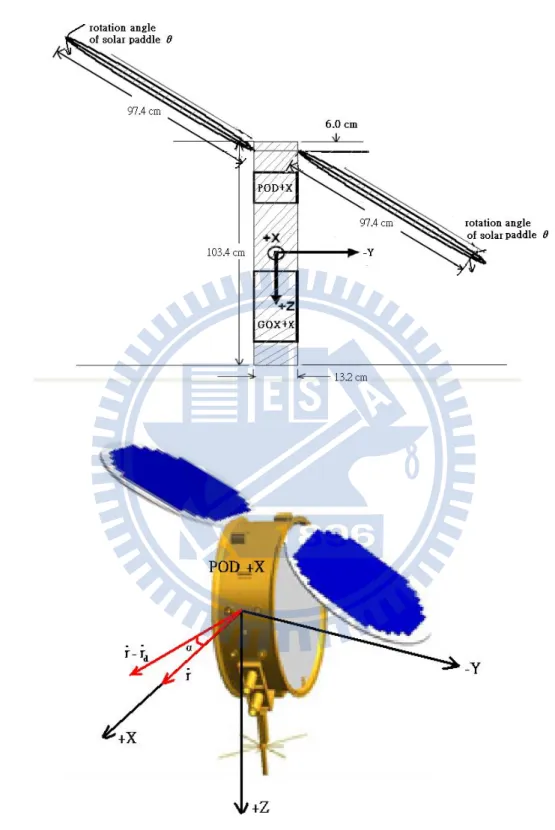
Fig. 3-1 The dimensions of the main part and solar panels of a COSMIC LEO (top),

velocity vector r& and LEO-to-atmosphere vector (r& −r&_d) (Hwang et al. 2008) ... 29

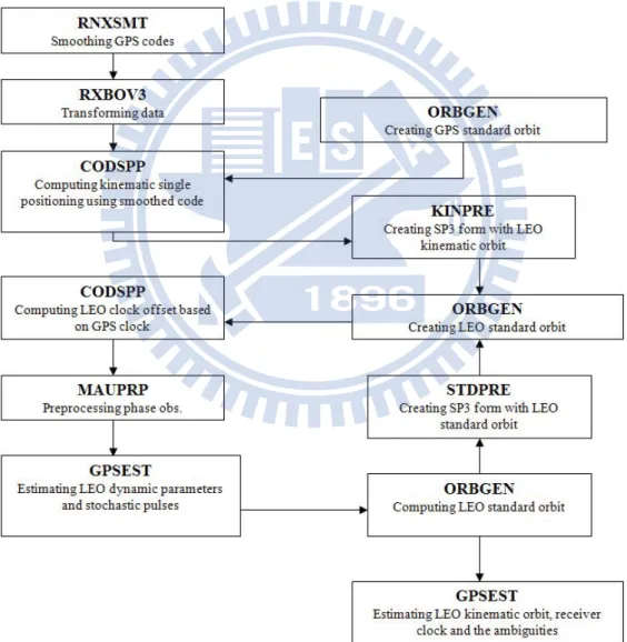
Fig. 3-2 Steps of precise kinematic orbit determination using GPS data ... 31

Fig. 3-3 Estimated atmospheric drag coefficients (top) and solar reflectivity coefficients

of FM 5 from Day 225 to 232, 2006 ... 37

Fig. 3-4 Raw and normal-point residuals in Y-direction (FM5, DOY216) ... 41

Fig. 4-1 Trajectory of FM5 satellite (August 2006) ... 44

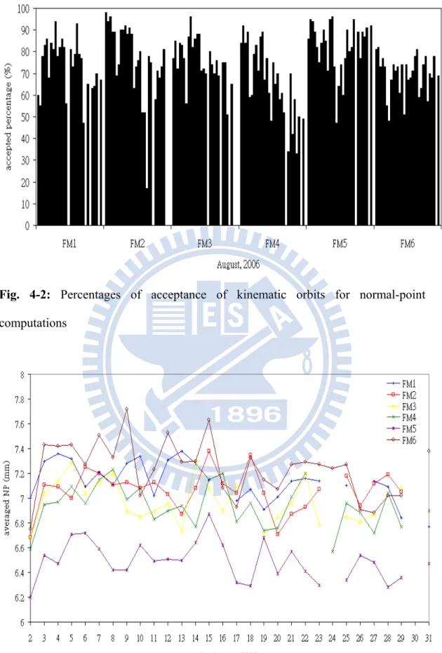
Fig. 4-2 Percentages of acceptance of kinematic orbits for normal-point computations .. 45

Fig. 4-3 Standard errors of normal-point kinematic orbits in August 2006 ... 45

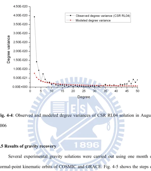
Fig. 4-4 Observed and modeled degree variances of CSR RL04 solution in August 2006

... 51

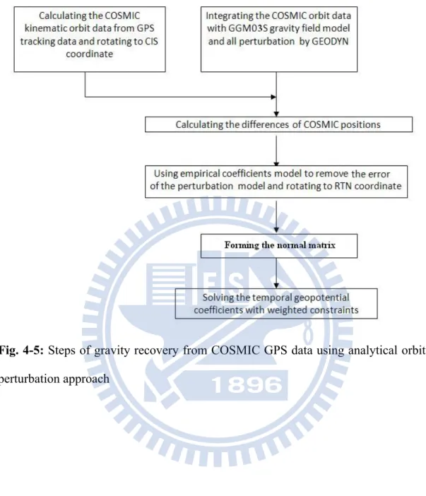
Fig. 4-5 Steps of gravity recovery from COSMIC GPS data using analytical orbital

Fig. 4-6 Degree variance and formal error degree variances of time-varying geopotential

coefficients from the COSMIC-only and COSMIC-GRACE solutions ... 56

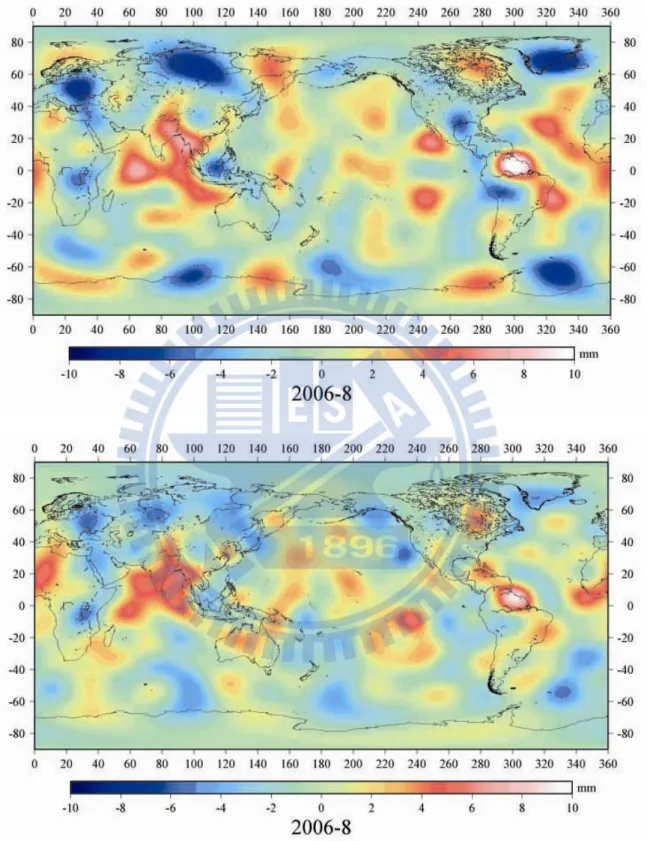
Fig. 4-7 Geoid variation to spherical harmonic degree 15 from the CSR RL04 solution

... 56

Fig. 4-8 Geoid variations to spherical harmonic degree 15 from COSMIC-only (top) and

COSMIC-GRACE solutions ... 57

Fig. 4-9 Relative differences of the COSMIC-only (top) and COSMIC-GRACE

coefficients with respect to the GRACE-derived coefficients of gravity variation for

nm

C

Δ (left) and ΔS_nm up to degree 15 ... 58

Fig. 4-10 Same as Fig. 4-9, but for the zonal coefficients ... 59

Fig. 4-11 Formal error degree variances of time-varying geopotential coefficients from

the CSR RL04 and the combined solutions ... 59

Fig. 4-12 Degree variances from COSMIC-GRACE, and calibrated error degree

variances from COSMIC-GRACE, GRACE and combined solutions ... 60

Fig. 4-13 Geoid variation to spherical harmonic degree 15 from the combined solution

... 61

Fig. 4-14 Geoid changes in Amazon area derived from combined (left) and GRACE

solutions ... 61

Fig. 5-1 RMS differences of GRACE-A (Top) and GRACE-B between NCTU kinematic

orbits and CSR dynamic orbits ... 64

Fig. 5-3 The simulation procedure of residual acceleration approach ... 72

Fig. 5-4 Recovered gravity variation using one week of one COSMIC data and degree-5

solutions by (a) oceanic mass variation (b) 1-cm white noise (c) 3-cm white noise (d) 5-cm white noise. Unit is mgal ... 73

Fig. 5-5 Relative differences of recovered zonal coefficients from the degree-5 solution

(one COSMIC satellite) ... 74

Fig. 5-6 Relative differences of the recovered harmonic coefficients of gravity variation

for (A) ΔCˆ_nm (degree-5 solution), (B) ΔSˆ_nm ( degree-5 solution), (C) ΔCˆ_nm

(degree-10 solution), (D) ΔSˆ_nm ( degree-10 solution), (E) ΔCˆ_nm (degree-15 solution), (F) ΔSˆ_nm ( degree-15 solution), (G) ΔCˆ_nm (degree-20 solution) and (H) ΔSˆ_nm ( degree-20 solution) using one week of six COSMIC satellite data with 3-cm white noise75

Fig. 5-7 Recovered gravity variation combining one week of six COSMIC satellite data

by adding 1-cm white noise (top), 3-cm white noise (center) and 5-cm white noise

(bottom). Unit is mgal ... 76

Fig. 5-8 Relative errors of the recovered harmonic coefficients up to degree 5 of gravity

variation for (A) ΔCˆ_nm (1 cm white noise), (B) ΔSˆ_nm (1 cm white noise), (C) ΔCˆ_nm

(3 cm white noise), (D) ΔSˆ_nm (3 cm white noise), (E) ΔCˆ_nm (5 cm white noise) and (F)

nm

Sˆ

Δ (5 cm white noise) using one week of six COSMIC satellites data ... 77

Fig. 5-9 Relative errors of recovered zonal coefficients from the degree-5 solution (six

geopotential coefficients from the COSMIC-only, COSMIC-GRACE and CSR RL04 solutions ... 81

Fig. 5-11 Geoid variations to spherical harmonic degree 15 from COSMIC-only solution

(top) and from COSMIC-GRACE solution using residual acceleration approach ... 82

Fig. 5-12 Geoid variation to spherical harmonic degree 15 from the combined solution

... 83

Fig. 5-13 Relative differences of the COSMIC-only (top) and COSMIC-GRACE

geopotential coefficients with respect to the CSR RL04 coefficients of gravity variation for ΔC_nm (left) and ΔS_nm up to degree 15 ... 84

Fig. 5-14 Relative differences of the combined solution coefficients with respect to the

CSR RL04 coefficients for ΔC_nm (left) and ΔS_nm up to degree 15 ... 85

Fig. 5-15 Relative differences for the zonal coefficients from ACC, AOP, CSR RL04 and

combined solutions ... 86

Fig. 5-16 Calibrated error degree variances from ACC, AOP, CSR RL04 and combined

solutions ... 87

Fig. 6-1 The monthly RMS differences between dynamic and kinematic orbits of

COSMIC and GRACE satellites in radial (top), along-track and cross-track (bottom) directions from September 2006 to December 2007 ... 91

Fig. 6-2 Maps of geoid variations up to degree 5 of CSR RL04 solutions from September

2006 to December 2007 ... 96

Fig. 6-4 Maps of geoid variations up to degree 5 of NCTU AOP solutions from

September 2006 to December 2007... 100

Fig. 6-5 Maps of geoid variations up to degree 5 of NCTU ACC solutions from

September 2006 to December 2007... 102

Fig. 6-6 Maps of geoid variations up to degree 15 of combined NCTU AOP solutions

from September 2006 to December 2007 ... 104

Fig. 6-7 Maps of geoid variations up to degree 15 of combined NCTU ACC solutions

from September 2006 to December 2007 ... 106

Fig. 6-8 Time series of ΔC₂₀ from CSR RL04 and SLR solutions from September 2006 to December 2007 ... 109

Fig. 6-9 Time series of ΔC₂₀ from SLR, CSR RL04, NCTU AOP and NCTU ACC

solutions from September 2006 to December 2007 ... 110

Fig. 6-10 Time series of delta ΔC₃₀ from CSR RL04, NCTU AOP, and NCTU ACC

solutions from September 2006 to December 2007 ... 110

Fig. 6-11 Time series of delta ΔC₄₀ from CSR RL04, NCTU AOP, and NCTU ACC

Chapter 1

Introduction

1.1 Background

The Earth’s gravity field is the sum of gravitational attraction and centrifugal force and it would vary in space and time due to the mass redistributions caused by atmospheric circulation, oceanic circulation, ground water-level variation, melting ice and other factors (Torge 1989). Gravity variations will result in satellite orbital perturbations, and variations in Earth rotational velocity and vertical datum of the Earth etc..

The precise Earth’s gravity field model can be applied to several disciplines of Earth sciences including geodesy, atmosphere, oceanography, aerospace engineering and geophysics. It can be determined with a variety of techniques and observation data types including surface gravity measurements, satellite tracking measurements and satellite radar altimetry measurements (Nerem 1995). Surface gravity measurements by terrestrial absolute/relative gravimetry, superconducting gravimetry, and airborne/ship-borne gravimetry can obtain the highest point-wise accuracy or regional information about the Earth’s gravity field. Satellite radar altimetry data can monitor the global sea surface height to derive gravity anomalies and geoid over the oceans or lake areas. Satellite tracking measurements are popular for global gravity field modeling and mainly acquired by Satellite Laser Ranging (SLR), Doppler Orbitography and Radio positioning Integrated by satellite (DORIS), Precise Range and Range Rate Experiment (PRARE), high-low satellite-to-satellite tracking (hl-SST), low-low satellite-to-satellite tracking (ll-SST) and Satellite Gravity Gradiometry (SGG).

Low Earth orbiters (LEOs) have become one of the basic and efficient tools for determining global time-varying gravity field in 21th century. A number of satellite missions have been launched in order to accomplish time-varying gravity field determination such as CHAMP (CHAllenging Minisatellite Payload) (Reigber et al. 1996), GRACE (The Gravity Recovery and Climate Experiment) (Tapley 1997), FORMOSAT-3/COSMIC (Constellation Observing System for Meteorology, Ionosphere and Climate) (Chao et al. 2000) and GOCE (Gravity Field and Steady-State Ocean Circulation Explorer) (ESA 1999). Although these missions employ different measurement techniques, the common feature of all missions is the use of GPS (Global Positioning System) observations for the precise orbit determination. The GPS-determined precise orbit data contains all information of orbital perturbation forces due to the Earth’s non-sphericity, air drag, solar radiation, N-body, solid Earth tide, ocean tide, Earth’s radiation (albedo), and relativistic effects (Seeber 2003). With appropriate methods removing the non-gravitational forces and constraints, the time-varying gravity can be derived from precise orbit data.

The FORMOSAT-3/COSMIC mission is a joint Taiwan-USA satellite mission launched in April 2006 for meteorological and ionospheric research and geodetic applications. Each of the six COSMIC satellites is equipped with two POD (Precise Orbit Determination) GPS antennas with a code-less, dual-frequency BlackJack GPS receiver (Dunn et al. 2003; Wu et al. 2005; Schreiner 2005; Montenbruck et al. 2006) developed by the Jet Propulsion Laboratory (JPL), which yield data for precise orbit and gravity determinations (Fig. 1-1). For abbreviation, the six COSMIC satellites will be named FM1- FM6, following the convention of NSPO (National Space Organization). With 6 satellites in the constellation, COSMIC configuration will provide a strong geometry in determining Earth’s gravity fields. COSMIC GPS data

can be used to compute orbit perturbations and/or accelerations so that they may recover the Earth’s temporal gravity fields and derive the spatial and time variations of the Earth’s mass. The origin of the spacecraft coordinate frame is at the geometric center of the ring. The angle between the line of coordinate origin- physical center of POD antenna and either the +X or -X axis is 30°. The angle between the normal to the antenna patch and the +X or –X axis is 15°. The COMs (center of mass) of the six satellites have been determined in a NSPO laboratory, in the configurations of full load and empty propellant fuel with stowed solar panels. The Attitude and Orbit

Control System (AOCS) of a COSMIC satellite is a combination of outputs from a

three-axis magnetometer, an one-axis Earth sensor and a three-axis Coarse Sun sensor but without the star-camera. The phase center offset and phase center variation (PCV) of the two POD antennas were both determined in an anechoic chamber using a mockup of COSMIC satellite, built by UCAR (the University Corporation for Atmospheric Research). The L1 and L2 phase centers were estimated for L1 and L2 frequencies and for 8 different solar arrays drive (SAD) orientations.

The geopotential parameters can be estimated from the LEO’s centimeter-precise POD data. The GPS data processing is performed at two stages for gravity recovery. In the first step, a reference orbit is computed from hl-SST data; the hl-SST data are applied to linearize the observational equations for the gravity coefficients estimation. In the second step, gravity recovery is carried out.Combining with different types of space measurements, the second step may use one of the three methods: (i) Kaula’s linear perturbation theory (Kaula 1966); (ii) direct numerical integration (Hwang 2001; Visser et al. 2001; Rowlands et al. 2002); (iii) energy balance approach (Wolff 1969; Wagner 1983; Jekeli 1999; Visser et al. 2003; Visser 2005).

The GRACE mission, a joint effort of NASA (USA) and DLR (German), was launched on March 17, 2002. This mission consists of two satellites, GRACE-A and GRACE-B, operating at an altitude of about 500 km as a formation at a distance of about 200 km apart. The orbit inclination is 89˚ as a near polar orbit and the period of 1 revolution is 94 minutes. The purpose of choosing such an orbit is mainly to obtain a homogeneous and complete global coverage for gravity field recovery. The primary objective of GRACE mission is to determine the high precision and high spatial resolution Earth’s gravity field, with an emphasis on its temporal changes (Tapley et al. 2004). The secondary objective is to determine total electron content and/or refractivity from the excess delay or bending angle of GPS measurements caused by the atmosphere and ionosphere. Both GRACE satellites are equipped with the following instruments: K-Band Ranging System (KBR), Accelerometer, GPS Space Receiver, Laser Retro-Reflector (LRR), Star Camera Assembly (SCA), Coarse Earth and Sun Sensor (CES), Ultra Stable Oscillator (USO) and Center of Mass Trim Assembly (CMT) (Fig.1-2) (GFZ homepage). The KBR system is to measure the inter-satellite distance forming the ll-SST observation, derived range-rates, and range-accelerations between two satellites. The accuracies of the inter-satellite distance and the range rate are 10μm and 1μm/s, respectively. On-board GPS TurboRogue Space Receivers receive GPS data to determine precise satellite orbits

and to synchronize time tags of KBR measurements. The SuperSTAR accelerometer

measures non-gravitational satellite accelerations. The satellite attitudes are controlled and determined by the SCA and CES systems. The LRR system is to measure distances between dedicated laser ground stations and the satellites with an accuracy of 1-2 cm. The USO system is built for the frequency generation of the KBR system. The CMT system is developed to adjust the offset between the satellite's COM and the

center of the accelerometer proof-mass.

Three alternative monthly GRACE gravity models published by different institutions CSR, GFZ and JPL are available at the web site of Center for Space Research (CSR), The University of Texas at Austin (http://www.csr.utexas.edu/grace). The static gravity solutions, GGM02S (Tapley et al. 2005) and GGM03S (Tapley et al. 2007) derived from GRACE KBR and GPS measurements, is also available at the website. The monthly solutions issued by CSR have three versions: Release 01 (RL01), Release 02 (RL02) and Release 04 (RL04). The CSR RL04 monthly solutions based on one-step variational equations approach contain fully normalized spherical harmonic coefficients up to degree and order 60. The solution is obtained through an optimally weighted combination of GPS and KBR data with one-day dynamic arcs for a designated month. More details of the RL04 model development can be found in the documents released with the GRACE products (Bettadpur 2007).

Fig. 1-1: A COSMIC spacecraft, payloads and spacecraft-fixed coordinate system, the

origin is at the center of the main body (cylinder) (Hwang et al. 2008)

Fig. 1-2: GRACE science instrumentation

1.2 Research objectives

The primary objective of this research is to develop efficient techniques and data processing procedures to process the hl-SST observations from COSMIC and GRACE to recover the temporal Earth’s gravity field models represented in the form of spherical harmonic series. Based on this objective,the first research regarding with the hl-SST data processing starts from a so-called analytical orbital perturbation (AOP) approach developed by Kaula (1966). For gravity recovery, the geometrically determined kinematic orbits are functions of orbit dynamic parameters, including geopotential coefficients, can be regarded as observations, and would be used in the least-squares estimation of these parameters.

The residual acceleration (ACC) approach is the second technique related to hl-SST data processing using satellites accelerations derived from precise kinematic and reference dynamic orbits by numerical differentiations. After removing accelerations other than the Earth’s gravity-induced accelerations, linear relations between LEO accelerations and gravity coefficients can be established. The residual acceleration differences between kinematic and reference orbits are assumed to be linear functions of time-varying geopotential coefficients and further used as observations for the geopotential coefficients estimation.

The second objective of this thesis is to derive time series of low-degree, zonal term gravity changes using COSMIC and GRACE GPS data. The combined COSMIC and GRACE solutions are also computed which are expected to enhance local temporal gravity signatures contained in the GRACE only solutions. The time series of zonal geopotential coefficients derived by AOP and ACC methods will also be assessed by those derived by tracking data.

1.3 Outline of Thesis

This dissertation comprises seven chapters. The detailed introductions of two gravity field recovery methods, analytical orbital perturbation approach and residual acceleration approach, are described in Chapter 2. This chapter starts from the analytical orbital perturbation approach which makes use of the relationship between the positional variations of orbits and variations in the six Keplerian elements from hl-SST observations. After that, the residual acceleration approach is proposed for gravity solutions.

In Chapter 3, since the precise orbits play an important role in gravity field recovery, the main principle of precise orbit determination is presented. The descriptions of orbit dynamics are discussed especially about the surface forces including atmospheric drag, solar radiation pressure and the Earth’s radiation pressure acting on COSMIC satellites. The procedures of precise dynamic orbit determination using GEODYN II software (Pavlis et al. 1996) and precise kinematic orbit determination using Bernese 5.0 software (Dach et al. 2007) are also provided. To reduce noises and data volume, the normal-point reduction is therefore introduced.

Chapter 4 is devoted to gravity field modeling using analytical orbital perturbation approach. The procedure of processing kinematic orbit and the orbit accuracy assessment is presented in this chapter. Both COSMIC and combined COSMIC and GRACE gravity solutions are computed using the post-processed orbit data.

Chapter 5 focuses on gravity field modeling derived from combined COSMIC and GRACE POD data and residual acceleration approach was applied. Position data screening and computation of residual accelerations are discussed in this chapter. The results from simulations and real data processing are carried out and compared with the results from AOP solution and CSR RL04 solution.

A time-series analysis of the estimated COSMIC and GRACE monthly low-degree temporal gravity solution is the subject of Chapter 6. The time span is from September 2006 to December 2007. The COSMIC and GRACE monthly low-degree temporal gravity solutions and combined solutions are presented in this chapter. Moreover, a comparison of some zonal geopotential coefficients with SLR and CSR RL04 solutions is also covered in this chapter.

Chapter 2

Methods for gravity field modeling using GPS observations

2.1 Introduction

A conventional one-step approach to model the gravity field is to use the raw GPS measurements directly in the equations of motion for estimation of geopotential coefficients. In this case, the relationship between geopotential coefficients and SST measurements is not linear, so the linearlization of observation equations is required. After linearization and with some iterations, the orbits of LEOs and GPS satellites and gravity field parameters can be determined by the method of least-squares adjustment with inputs from GPS ground and space-borne data, SLR data, accelerometer data, K-band observation data, etc. (Zhu et al 2004). The GGM and EIGEN series of static gravity field models based on GRACE KBR and GPS measurements are computed in this way (Tapley et al. 2004; Reigber et al. 2005; Förste et al. 2006).

At present, the two-step approach, i.e. computing orbit first and estimating gravity fields using such orbits, is widely adopted for gravity field modeling. Compared to the one-step approach, this two-step procedure avoids the time-consuming computations of associated partials with respect to parameters. Two basic important physical laws are applied: the energy conservation law and Newton’s second law of motion. In this thesis, we focus on the two-step approach using GPS observations based on Newton’s second law of motion. See Section 2-2 for the description of the two-step approach where the analytical orbital perturbation approach is involved (Kaula 1966). The residual acceleration approach linking the acceleration vector to the gradient of the gravitational potential is discussed in Section 2.3.

2.2 Theory of analytical orbital perturbation approach

To establish the linear relationship between the satellite positions and geopotential coefficients, Kaula (1966) demonstrated the analytical orbital perturbation method for gravity field recovery in terms of the six Keplerian elements. The six Keplerian elements (a ,e ,i ,ω ,Ω ,M ) are semi-major axis, eccentricity, inclination, argument of perigee, right ascension of the ascending node, and mean anomaly. To use the three-dimensional positional data for gravity field recovery, orbital perturbations in radial, along-track and cross-track (RTN) directions should be transformed to perturbations in the Keplerian elements.

The radial distance r of a LEO from the geocenter is ) cos 1 ( e E a r= − (2-1)

where E is eccentricity anomaly, which is related to the mean anomaly by

E e E

M = − ⋅sin . The perturbations in the RTN directions, shown in Fig. 2-1, can be expressed as E E ae e E a a E e E E r e e r a a r x Δ = − Δ − Δ + Δ ∂ ∂ + Δ ∂ ∂ + Δ ∂ ∂ =

Δ ₁ (1 cos ) ( cos ) ( sin ) (2-2)

] ) (cos [ ) cos ( 2 = Δ +ΔΩ = Δ +Δ + ΔΩ Δx r u i r ω f i (2-3) ] ) cos (sin ) [(sin 3 = Δ − ΔΩ Δx r u i i u (2-4)

Fig. 2-1: Geometry showing the effects of perturbations in argument of perigee (top),

The potential due to the Earth (called geopotential) at the satellite position, V, is expanded into a spherical harmonic series as (Heiskanen and Moritz 1985)

ns K n n m nm nm nm n e V r GM P m S m C r a r GM r V + = ⎥ ⎦ ⎤ ⎢ ⎣ ⎡ _{+ +} =

∑

∑

= = 1 0 ) (sin ) sin cos ( ) ( 1 ) , , ( φ λ λ λ φ (2-5)

where (r,φ,λ) are the spherical coordinates (radial distance, geocentric latitude and longitude), ae is the semi-major axis of the Earth’s reference ellipsoid, K is the

maximum degree of expansion depending on the satellite altitude, (C_nm,S_nm) _are geopotential coefficients, P is the fully normalized associated Legendre function of _nm

degree n and order m, and V is the potential due to the Earth’s non-sphericity _ns

(perturbing potential). From eq. (2-5), the perturbing potential V can be expressed _ns

in terms of the six Keplerian elements as (Kaula 1996; Balmino 1994; Hwang 2001):

∑∑∑ ∑

= = = =− = = K n n m n p Q Q q nmpq ns R R V 2 0 0 (2-6) ) , , , ( ) ( ) ( 1 ω Ωθ = ₊ F i G e S M a GMa R _{n nmp npq nmpq} n e nmpq (2-7)

where Q is the number depending on the orbital eccentricity, and θ is Greenwich sidereal time (GST). F_nmp is the fully normalized inclination function, and is defined

nmp nm nmp H F F = (2-8) where { } { }

∑

− − − − = − ⎟ ⎠ ⎞ ⎜ ⎝ ⎛ − + ⎟⎟ ⎠ ⎞ ⎜⎜ ⎝ ⎛ − − ⎟⎟ ⎠ ⎞ ⎜⎜ ⎝ ⎛ − − × − + − = n m n p m p n j a a n j n m n E nmp c s j m n p j p n p n p m n i F 2 2 , min 0 , 2 max 2 2 1 2 2 2 ) 1 ( )! ( ! 2 )! ( ) 1 ( ) ( (2-9)

[

]

1/2 )! /( )! )( 1 2 ))( ( 2 ( m l l m l m H_nm = −δ − − + (2-10) ) 2 / cos(i

c= , s=sin(i/2), and a=m−n+2p+2j_. G_npq(e) is the eccentricity function, which is a polynomial of e about the order e (Kaula 1966). q S_nmpq is defined by ) sin( ) cos( ) , , , ( _nmpq nm nm nmpq nm nm nmpq C S S C M S ω θ ψ _⎟⎟ ψ ⎠ ⎞ ⎜⎜ ⎝ ⎛ + ⎟⎟ ⎠ ⎞ ⎜⎜ ⎝ ⎛ − = Ω +₋ +₋ (2-11) ) ( ) 2 ( ) 2 ( ω θ ψ = n− p + n− p+q M +m Ω− (2-12)

where C is _nm+ C when (n-m) is even and _nm C is _nm− C when (n-m) is odd (the _nm

same is true for S ). _nm

M R a n dt da ∂ ∂ = 2 ω ∂ ∂ − − ∂ ∂ − = R e a n e M R e a n e dt de 2 2 2 2 ₁ 1 Ω ∂ ∂ − − ∂ ∂ − = R i e a n R i e a n i dt di sin 1 1 sin 1 cos 2 2 2 2 ω (2-13) e R e a n e i R i e a n i dt d ∂ ∂ − + ∂ ∂ − − = ₂ 2 2 2 1 sin 1 cos ω i R i e e a n dt d ∂ ∂ − = Ω sin 1 1 2 2 a R a n e R e a n e n dt dM ∂ ∂ − ∂ ∂ − − = 1 ₂2 2

where _{n= GM/ a}3 _{is the mean angular velocity. An approximate solution of eq.}

(2-13) with a closed form can be derived for a near-circular orbit (e≈0).In such a solution, it is assumed that a , and i are invariant with time (denoted as e a , and e

i ) and ω ,Ω and M vary linearly with time, so that (Hwang and Hwang 2002)

( )

(

)

( )

(

)

( )

0

(

0

)

0 0 0 0 t t M M t M t t t t t t − + = − Ω + Ω = Ω − + = & & & ω ω ω (2-14)

linear rates. Because the C term (or 20 −J2) is the order of 10 3 −

and it is at least 1000 times larger than any other geopotential coefficients, the major contribution to the perturbing potential is due to this term and can be expressed as

(

)

∑ ∑

= ∞ −∞ = + − + − ⎟ ⎠ ⎞ ⎜ ⎝ ⎛ = 2 0 2 20 2 20 20 () ( )cos(2 2 ) (2 2 ) p q pq p e _{F i G e p p q M} a a a GMC R ω (2-15)

The term with M in eq. (2-15) has a period much smaller than other terms, and hence

can be neglected provided that long-period perturbations are sought, that is,

0 2

2− p+q= (2-16)

The (p, q) terms with (0, -2) and (2, 2) do not exist (Kaula 1966), thus the only term left is ) ( ) ( ₂₁₀ 201 2 20 2010 F i G e a a a GMC R e_⎟ ⎠ ⎞ ⎜ ⎝ ⎛ = (2-17)

Based on Kaula (1966), the values of F₂₀₁(i) and G₂₁₀(e) are

2 3 2 210 2 201 ) 1 ( ) ( 2 / 1 4 / sin 3 ) ( − − = − = e e G i i F (2-18)

0 = = = dt di dt de dt da (2-19)

(

i

)

a e a nC dt d _e 2 2 2 2 20 _{1 5cos} ) 1 ( 4 3 ₋ − = = ω ω_& i a e a nC dt d _e cos ) 1 ( 2 3 2 2 2 20 − = Ω = Ω& (2-20)

(

3cos 1

)

) 1 ( 4 3 2 2 2 20 ₋ − − = = i a e a nC n dt dM M& e

A reference orbit at the reference epoch t based on nine orbital parameters ₀

(a ,e ,i ,ω₀ ,Ω₀ ,M₀ ,ω& ,Ω& ,M& ) is used. Integrating eq. (2-13) with respect to time yields

∑∑∑ ∑

= = = =− Δ = Δ K n n m n p Q Q q nmpq 2 0 0 α α (2-21)

where α denotes any of the six Keplerian elements. Integrating eq. (2-11), we get

) cos( ) sin( ) , , , ( * nmpq nm nm nmpq nm nm nmpq C S S C M S ω θ ψ _⎟⎟ ψ ⎠ ⎞ ⎜⎜ ⎝ ⎛ − ⎟⎟ ⎠ ⎞ ⎜⎜ ⎝ ⎛ − = Ω +₋ +₋ (2-22)

The perturbations in a ,e ,i are

∑∑∑ ∑

= = = =− = Δ K n n m n p Q Q q nmpq i nmpq k S s 2 0 0 α (2-23)

∑∑∑ ∑

= = = =− = Δ K n n m n p Q Q q nmpq i nmpq k S s 2 0 0 * α (2-24) The coefficients i nmpq

α in the order of six Keplerian elements a ,e ,i,ω,Ω,Mare

] 2 ) 2 ( ) 1 [( ) 1 ( ) 2 ( 2 2 / 1 2 2 / 1 2 2 1 p n q p n e G F e e b q p n G F ab npq nmp nmpq npq nmp nmpq + − + − − × − = + − = α α 2 / 1 2 ' 4 2 / 1 2 3 ) 1 ( sin ) 1 ( sin cos ) 2 [( e I G F b e I m I p n G F b npq nmp nmpq npq nmp nmpq − = − − − = α α (2-25) ⎥ ⎥ ⎦ ⎤ ⎢ ⎢ ⎣ ⎡ + − − − − + = ⎥ ⎦ ⎤ ⎢ ⎣ ⎡ − − − = nmpq npq npq npq nmp nmpq npq nmp npq nmp nmpq n q p n G G e e G n F b G F e I I G F e e b ψ α α & ) 2 ( 3 ) 1 ( ) 1 ( 2 ) 1 ( sin cos ) 1 ( ' 2 / 1 2 6 ' 2 / 1 2 ' 2 / 1 2 5 where n e nmpq a a n b ⎟ ⎠ ⎞ ⎜ ⎝ ⎛ = ψ& (2-26) ) ( ) 2 ( ) 2 ( ω θ

e G G i F F npq npq nmp nmp _∂ ∂ = ∂ ∂ = ' ' _{, (2-28)}

where ψ& is the frequency of the perturbations, and θ& is the velocity of the GST ( about _7.292115×10−5_{rads ).} −1

Let Δ and x_i Δ represents the perturbations in the RTN directions and of the s_k

six Keplerian elements. We have

3 , 2 , 1 , 6 1 = Δ = Δ

∑

= i s c x k k i k i (2-29) where i k

c are the coefficients used to transform the Keplerian perturbations to the

RTN perturbations (Hwang 2001). The coefficients are , cos 1 sin , cos 1 sin cos , cos 1 , 0 1 6 2 1 2 1 1 1 5 1 4 1 3 E e E ae c E e E ae E a c E e c c c c − = − + − = − = = = = , ) cos 1 ( 1 , , cos , ) cos 1 ( 1 sin ) cos 2 ( , 0 2 2 2 6 2 5 2 4 2 2 2 2 3 2 1 2 1 E e e r c r c I r c E e e E E e e r c c c − − = = = − − − − = = = (2-30) , cos 1 sin sin 1 ) (cos cos sin , cos 1 ] sin cos 1 ) (cos [sin , 0 2 3 4 2 3 3 3 6 3 5 3 2 3 1 E e E e e E I r c E e E e e E r c c c c c − − − − = − − − − = = = = = ω ω ω ω

The above relationships between orbit perturbations and geopotential coefficients can be used for least-squares estimation of the later given GPS-determined satellite orbits.

2.3 Theory of residual acceleration approach

A residual acceleration method is employed to determine the time variation of the Earth’s gravity field. In this method, the accelerations of LEOs are determined by numerical differentiations of the positions of LEOs. All perturbing forces caused by the static gravity field, Earth's non-sphericity, N-body, solid Earth tide, ocean tide, air drag, solar radiation pressure, Earth radiation and relativity are modeled first. After removing accelerations other than the Earth’s gravity-induced accelerations, linear relations between LEO accelerations and gravity coefficients can be established. Empirical parameters can be used to model the residual non-gravitational accelerations.

The total gravitational force is the gradient of V. The acceleration vector expressed in the Earth-fixed coordinate system is (GSFC 1989)

⎥ ⎥ ⎥ ⎥ ⎥ ⎥ ⎦ ⎤ ⎢ ⎢ ⎢ ⎢ ⎢ ⎢ ⎣ ⎡ ∂ ∂∂ ∂∂ ∂ ⎥ ⎥ ⎥ ⎥ ⎥ ⎥ ⎥ ⎦ ⎤ ⎢ ⎢ ⎢ ⎢ ⎢ ⎢ ⎢ ⎣ ⎡ ∂ ∂ ∂ ∂ ∂ ∂ ∂ ∂ ∂ ∂ ∂ ∂ ∂ ∂ ∂ ∂ ∂ ∂ = ⎥ ⎥ ⎥ ⎥ ⎥ ⎥ ⎥ ⎦ ⎤ ⎢ ⎢ ⎢ ⎢ ⎢ ⎢ ⎢ ⎣ ⎡ ∂ ∂∂ ∂∂ ∂ =

λ

φ

λ

φ

λ

φ

λ

φ

ns ns ns b b b b b b b b b b ns b ns b ns b ns V Vr V z z z r y y y r x x x r z V y V x V a _(2-31)

where xb , yb and zb are the Earth-fixed coordinates and r,φ , and λ are the spherical

coordinates. The partial derivatives of the non-spherical portion of the Earth’s potential with respect to r,φ , and λ are given by

∑

∞

∑

= =

+

+

⎟

⎠

⎞

⎜

⎝

⎛

−

=

∂

∂

2 0

2

(

1

)

(

cos

sin

)

(sin

)

n n m nm nm nm n e ns

_n

_C

_m

_S

_m

_P

r

a

r

GM

r

V

_λ

_λ

_φ

(2-32)

[

( )( 1)/(1 ( )) (sin ) tan (sin )

]

) sin cos ( 1 , 0 2

φ

φ

φ

δ

λ

λ

φ

nm m n n m nm nm n n e ns P m P m m n m n m S m C r a r GM V − + + + − ⋅ + ⎟ ⎠ ⎞ ⎜ ⎝ ⎛ = ∂ ∂ + = ∞ =

∑

∑

(2-33)

)

(sin

)

sin

cos

(

0 2

φ

λ

λ

λ

nm n m nm nm n n e ns

_m

_S

_m

_C

_m

_P

r

a

r

GM

V

∑

∑

= ∞ =

−

⎟

⎠

⎞

⎜

⎝

⎛

=

∂

∂

(2-34)

where δ(m)=1 when m is zero and δ(m)=0 when m is not zero. Substituting eq. (2-32) through eq. (2-34) into eq. (2-31) and transforming the Earth-fixed coordinates (xb , yb , zb) into the spherical coordinates (r , φ , λ), eq. (2-31) can be rewritten as

Ma a = ⎥ ⎥ ⎥ ⎥ ⎥ ⎥ ⎦ ⎤ ⎢ ⎢ ⎢ ⎢ ⎢ ⎢ ⎣ ⎡ ∂ ∂∂ ∂∂ ∂ ⎥ ⎥ ⎥ ⎥ ⎥ ⎥ ⎥ ⎥ ⎦ ⎤ ⎢ ⎢ ⎢ ⎢ ⎢ ⎢ ⎢ ⎢ ⎣ ⎡ + + + − + − + − =

λ

φ

φ

cos 0 2 2 2 2 2 2 2 2 2 2 r V r Vr V r y x r z y x x y x r z y r y y x y y x r z x r x ns ns ns b b b b b b b b b b b b b b b b b b b b ns (2-35)

where a is the acceleration vector

[A

_r

,

A

_φ

,

A

_λ

]

expressed in a local rotating frame which are the radial, latitudinal, and longitudinal accelerations, respectively. M is an orthogonal matrix. The transformation of eq. (2-35) can be simplified by neglecting precession, nutation, and polar motion to obtain the acceleration vector _aI _{in the}

⎥ ⎥ ⎥ ⎥ ⎥ ⎥ ⎦ ⎤ ⎢ ⎢ ⎢ ⎢ ⎢ ⎢ ⎣ ⎡ ∂ ∂∂ ∂∂ ∂ ⎥ ⎥ ⎥ ⎥ ⎥ ⎥ ⎥ ⎥ ⎦ ⎤ ⎢ ⎢ ⎢ ⎢ ⎢ ⎢ ⎢ ⎢ ⎣ ⎡ + + + − + − + − = − λ φ φ cos 0 1 2 2 2 2 2 2 2 2 2 2 r V r Vr V r y x r z y x x y x r yz r y y x y y x r xz r x ns ns ns I a _(2-36)

where x, y and z are the inertial coordinates, 2 2 2

z y x

r = + + . The longitude and

latitude are calculated as follows:

− = _tan−1_(y/x)

λ

GAST (2-37) ) / ( sin−1 _{z r} =

φ

(2-38)

Chapter 3

Force modeling and precise orbit determination for COSMIC

3.1 Introduction

Precise orbits of a satellite position are important for positioning the satellite and for estimation of the Earth’s gravitation. Owing to the development of GPS, the spacecraft equipped with hl-SST receiver can collect position data continuously. The dynamic method (using force models) and the kinematic method (not using force models) (Švehla and Rothacher 2003; Jäggi et al. 2006 and 2007; Hwang et al. 2009) are two popular methods using GPS data applied for POD of LEOs. In addition, the so-called reduced-dynamic orbit determination, which is a compromising method between the dynamic method and the kinematic method, requires simplified force models. All above procedures for POD require GPS satellite ephemeris, Earth rotation information, and LEO GPS observation data as input for processing.

In Section 3.2, we focus on the perturbation force models acting on a COSMIC spacecraft. Without an accelerometer on the COSMIC spacecraft, the non- gravitational accelerations due to atmospheric drag and solar radiation need to be modeled. Section 3.3 and 3.4 describe the kinematic and dynamic orbit determination methods, complete with the principles, computation procedures and some analysis of results. The procedure of observed orbit data compression applied in gravity recovery is presented in the last part of this chapter.

3.2 Orbit dynamics of COSMIC satellite

The perturbing forces (accelerations) can be classified into gravitational forces and surface forces (or non-gravitational forces). The gravitational forces include the

Earth’s non-sphericity, N-body, solid Earth tide, ocean tide, and relativistic effect, and the surface forces include atmospheric drag, solar radiation pressure and the Earth’s radiation pressure. General accelerations, or empirical accelerations, are used to absorb the mis-modeled and un-modeled gravitational and surface forces. The algorithms of N-body, solid Earth tide, ocean tide, and relativistic effects can be found in a standard textbook of orbit dynamics such as Seeber (2003), and they will not be elaborated here. In this section, we focus on the parameters related to Earth’s non-sphericity, atmospheric drag and solar radiation pressure.

3.2.1 Equations of motion and perturbing potential force

In a geocentric inertial rectangular coordinate system, the equations of motion of an artificial Earth satellite such a COSMIC spacecraft can be expressed as (Long et al. 1989; Montenbruck and Gill 2001; Seeber 2003)

Pert ns a a r r =− ₃ + + r GM && (3-1) where

r_{: vector of satellite coordinates in the inertial frame}

r&&_{: acceleration vector}

GM: Earth’s gravitational constant

ns

a _{: acceleration due to Earth’s non-sphericity}

Pert

The first term in eq. (3-1) is called the point mass effect of the Earth given by Newton’s law of gravity and is 1000 times larger than any other acceleration. Eq. (3-1) contains a system of second order differential equations which can be integrated to obtain the satellite positions and velocity at any epoch giving the initial state vector. The direct integration known as Cowell’s method (Balmino 1989) is selected for the simplicity and capacity for incorporating additional perturbations easily (Pavlis et al. 1996). The accelerations in eq. (3-1) are associated with certain parameters and can be adopted from existing values or estimated by satellite tracking data.

The acceleration a_{earth due to the geopotential is the gradient vector of the}

geopotential: ns earth r a r a =− + ∂ ∂ = ₃ r GM V (3-2)

The first term in eq. (3-2) corresponds to the potential of a spherically symmetric Earth and the potential can be considered static. In fact, due to mass re-distribution in the Earth system, the geopotential is time-dependent so that the time-varying part should be considered. This is equivalent to dividing the coefficients in eq. (2-5) into a static part and a time-varying part as

) ( ) ( , ) ( ) (_{t C}0 _{C t S t S}0 _{S t} C_nm = _nm+Δ _{nm nm} = _nm+Δ _{nm (3-3)}

time-varying coefficients(ΔC_nm(t),ΔS_nm(t)) with respect to a mean gravity field.

3.2.2 Atmospheric drag and solar radiation effects on COSMIC satellites

The acceleration vector of a LEO due to atmospheric drag is given by

) r r ( r r

a_drag =− &−&_d &−&_d

m A C d Dρ 2 1 (3-4)

where CD is drag coefficient depending on the LEO shape and atmospheric

composition, ρ is atmospheric density at the LEO position, Ad is effective

(cross-sectional) area and m is the mass of the LEO, r r& &, _d are the velocity vectors of

the LEO and atmosphere in the inertial frame, and (r& −r&_d) is the velocity vector of the LEO relative to atmosphere. For each of the six COSMIC spacecrafts, the mass (with full thrust fuel) has been determined in the chamber test before the launch (April 2006). The remaining thrust fuel during the flight is observed and is used to adjust the time-dependent mass after the launch (Hwang et al. 2006 and 2009). The effective area Ad is the projected area of the area of the satellite in the flight direction

onto a plane perpendicular to the direction(_{r && −}r_d). A COSMIC spacecraft travels in a manner that the POD+X antenna points to the flight direction (Fig. 3-1). Therefore, the total area in the flight direction is

panel main

T A A

A = +

where Amain is the area of the main body and Apanel is the area of two solar panels,

which are computed as

) (m sin ) 2 974 . 0 ( 2 ) (m 132 . 0 034 . 1 2 2 2 θ π × = × = panel main A A (3-6)

where θ is the rotational angle of the solar panel (Fig. 3-1). Here we assume the thickness of the solar panels is negligible. The effective area was then computed by

) ( cos1 d d)/rr r r r (

r&⋅ &−& & &−&

= − T d A A (3-7) The velocity vector of atmosphere was computed as

⎥ ⎥ ⎥ ⎦ ⎤ ⎢ ⎢ ⎢ ⎣ ⎡ − − = 0 x y h h ω ω d r& (3-8)

where x and y are geocentric coordinate components of the LEO in the inertial frame, and ω_h is the rotational velocity of atmosphere at an altitude of h computed as (King-Hele and Walker 1983)

) 10 917401 . 3 10 108229 . 5 10 88539 . 1 10 588187 . 1 1 ( 4 11 3 8 2 5 3 h h h h e h − − − − × + × − × + × − =ω ω (3-9)

where ω_e is the mean rotational velocity of the Earth (7.292115_×10−5rad/sec_{), and}

h is in km.

The acceleration vector due to solar radiation pressure is

3 2 ) ( s s srp r r r r a − − = au m A C P s r s ν (3-10)

where ν is the eclipse factor, Ps is solar flux at one astronomical unit (au)

(_{4.560 10×} −6_N/m2_{), C}

r is reflectivity coefficient depending on the characteristics of

the LEO, As is the effective area (different from the effective area for atmospheric

drag) and r is the position vector of the Sun. The method to compute the effective _s

area for the solar radiation pressure is the same as that used in the atmospheric drag. In this case, the effective area lies in a plane perpendicular to the vector (r− ). Cr_s r

can be expressed as (1+ε), where ε is reflectivity (from 0 to 1), which depends on the material of satellite parts. The eclipse factor depends on the position of LEO; ν=0 when the LEO is in the Earth’s shadow, and ν=1 when the LEO is illuminated by the Sun. The orbit dynamic modeling software we used is able to determine the eclipse factor in the cases of umbra and penumbra based on the ratio of the sunlight received at the LEO location, so that in practice the eclipse factor for a COSMIC satellite varies from zero to one.

Fig. 3-1: The dimensions of the main part and solar panels of a COSMIC LEO (top), velocity vector r& and LEO-to-atmosphere vector (r_{& −}r_&d) (Hwang et al. 2008)

3.3 Kinematic orbit determination using Bernese 5.0

The precise kinematic orbits of LEOs in this research were determined by the

Bernese Version 5.0 GPS software (Dach et al. 2007). The reduced dynamic and

kinematic approaches are available in Bernese 5.0 for POD with GPS observations.

The reduced dynamic approach estimates orbit arc-dependent parameters including the initial state vector (6 Keplerian elements), 9 solar radiation coefficients and three stochastic pulses in the radial, along-track and cross-track directions. The kinematic approach estimates the kinematic parameters of an orbit arc, including epoch coordinate components, receiver clock errors and phase ambiguities. Both the reduced dynamic and kinematic orbit determinations require high precision GPS satellite

orbits and clocks. The GPS satellite precise orbits and high-rate clocks can be downloaded on the website provided by the Center for Orbit Determination in Europe (CODE, http://www.aiub.unibe.ch/igs.html). In the kinematic orbit determination with Bernese 5.0, the reduced dynamic orbit serves as a priori orbit for the kinematic orbit.

Fig. 3-2 shows the steps of precise kinematic orbit determination using real GPS data. The zero-differenced ionosphere-free GPS measurements are usually used for point-wise calculation of the satellite positions in the kinematic approach. The limitations of orbit accuracy associated with kinematic orbits are based on the GPS satellite observation numbers and relative GPS-LEO geometry (Byun and Schutz 2001). Satellite coordinates are estimated together with one GPS receiver clock

parameter every epoch. Comparing with SLR observations, the kinematic POD with accuracy of 1–3 cm was demonstrated for the GRACE mission (Švehla and Rothacher

2004).Using an overlapping analysis, the orbit accuracy of COSMIC is about 3 cm, compared to 1 cm in the case of GRACE satellites (Hwang et al. 2009). We find that the quality of GPS data depends on the quality of satellite attitude data. For the case

measurements over the equator and the polar regions are _0.5o _{and 3}o

, respectively, and are larger at a lower altitude. When the attitude of a satellite is poorly determined, the uncertainties in the estimated GPS phase ambiguities are relatively large, leading to degraded orbital accuracy. The detail of GPS-determined orbits of GRACE and COSMIC satellites using the kinematic approaches by Bernese have been documented by Švehla and Rothacher (2005), Jäggi et al. (2007) and Hwang et al. (2009).

3.4 Dynamic orbit determination using GEODYN II software

The dynamic orbit determination strategy for LEO based on GPS double- difference tracking data is demonstrated for the first time for TOPEX/Poseidon mission (Bertiger et al. 1994; Schutz et al. 1994). The equations of motion are solved by numerical integration. The dynamic model errors will lead to systematic errors growing with the arc length (Bock 2003).

In this research, we use NASA Goddard GEODYN II software to model the perturbing forces described in Section 3.2.1. GEODYN II is used extensively for satellite orbit determination, geodetic parameter estimation, tracking instrument calibration, satellite orbit prediction, as well as for other applied research in satellite geodesy using virtually all types of satellite tracking data (Pavlis et al. 1996). For direct numerical integration, GEODYN II uses Cowell’s summation method to obtain the position and velocity at epoch and uses the Bayesian’s least-squares method for parameter estimation. The mathematical models of the perturbing forces used in GEODYN II can be found in Long et al. (1989), Pavlis et al. (1996) and McCarthy (1996). GEODYN II has been used for precise orbit determination/prediction and force modeling in various Earth resource satellites such as TOPEX/Poseidon and GRACE. Temporal gravity fields from such satellite tracking data as SLR and GRACE KBR have been derived with GEODYN II (Cox and Chao 2002; Luthcke et al. 2006).

GEODYN II is divided into three major components: the Tracking Data Formatter (TDF), GEODYN IIS and GEODYN IIE. The flow of running GEODYN II can be found in Hwang (2002). The TDF program takes in the one of several tracking data forms. In this research, the tracking data format is PCE data format containing the information of satellite position and velocity as a priori orbit.

In preparation for the execution of GEODYN II, a file containing the ephemeris of the planets and a file containing A1UTC, polar motion, solar flux and magnetic flux must be made ready. A1UTC is the difference between the atomic time (A1) used in GEODYN II and the universal time (UTC), which is available from http://hpiers.obspm.fr/eop-pc/. Solar flux and magnetic flux are obtained from NOAA’s web site ftp://ftp.ngdc.noaa.gov under the directory STP/ GEOMAGNETIC_DATA/INDICE. These raw data are processed to produce binary files suitable for input to GEODYN IIS program.

The GEODYN IIS program is mainly used to read and process the option cards, the input observation data, optional gravity model, station geodetics, area/mass files, ephemeris and table data. The default gravity model is stored in the file ftn12. In this research, we choose GGM03S gravity models up to degree/order 70 derived from GRACE GPS and KBR observations.

The JPL export ephemeris as input file ftn01 is used in GEODYN IIS for nutations, positions, and velocities of the Moon, Sun, and planets. In this research, we use the JPL binary DE-403 ephemeris. GEODYN II interpolates for the ephemeris in the mean of 1950.0 reference system by Chebyshev interpolation. This step gives greater accuracy than interpolating in the reference system (the true of date coordinate system) because the high-frequency perturbations due to nutations are absent. After interpolation, the coordinates are then rotated to the true of date system using the precession and nutation matrices (Seeber 2003). More details on the transformations between different coordinate systems can be found in the textbooks or manuals like Long et al. (1989), Pavlis et al. (1996) and Seeber (2003).

The file ftn05 contains all option cards determining the force and non-force model parameters to be used in the program execution. These option cards are divided

2002). The Global Set consisting of four groups provides all of the common arcs processing information. The first group, Global Set Mandatory Cards, is the mandatory run description on other three cards. The second set of Global Set Option cards is used to define and/or estimate conditions which are common to all the arcs being processed. This group contains the information and estimations of the Earth's gravitational potential and/or new Earth constants, application and/or adjustment of time dependent gravity coefficients, dynamic polar motion, the third body gravitational potential and/or new constants, solid Earth tide model, ocean tide model, atmosphere drag model, solar flux, and tectonic plate motion. The third group is the Position Card Group containing the information of tracking stations. The last group is the Global Set Terminator to end the Global Set.

One or more Arc Set contains information defining its arc in ftn05 file. The Arc Set also has four groups in this order. The first group, Arc Set Mandatory Cards, is to decide the reference coordinate system and time and spacecraft parameters in this arc. The second group, Arc Option Set cards, is specified to make use of GEODYN II's individual arc capabilities. The third group is the Data Selection/Deletion Subgroup used to edit input observations. The last group is the Arc Set Terminator to end the Arc Set.

The parameters in the Global Set for the force models of COSMIC given in Table 3-1 are defined by input option cards in the file ftn05. For surface forces in the Arc set, we solve for atmospheric drag coefficient, radiation coefficient and 9 empirical coefficients of general acceleration along the radial, along-track and cross-track directions every 1.5 hours (one orbital period) using COSMIC kinematic orbits. As an example, Fig. 3-3 shows the estimated atmospheric drag coefficients and reflectivity coefficients for FM5. These estimated coefficients vary over time, and the

and 1.23/0.30, respectively. The general accelerations for COSMIC (Table 3-1) at an

altitude of 520 km are on the order of 10-11ms-2 . GEODYN IIE performs the

computation of satellite orbit and geodetic parameter estimations. The output from IIE contains all necessary information for data analysis.

The main purpose of precise dynamic orbit determination is to generate a reference orbit to compute the residual orbit perturbations for gravity field recovery. The residual orbit perturbation is a function of the perturbing force due to the perturbing geopotential. Like satellite position, satellite acceleration contains the effect due to the geopotential, plus other perturbing forces which must be modeled for gravity field recovery.