高效能且低成本之可參數化快速傅利葉轉換硬體產生器

(1)

國立交通大學

電子工程學系

電子研究所

碩

士

論

文

高效能且低成本之可參數化快速傅利葉轉

換硬體產生器

A Parameterizable Generator for High-Performance and

Low-Cost FFT Cores

研究生：王毓翔

(2)

高效能且低成本之可參數化快速傅利葉轉換

硬體產生器

A Parameterizable Generator for High-Performance

and Low-Cost FFT Cores

研究生：王毓翔 Student: Yu-Hsiang Wang

指導教授：周景揚教授 Advisors: Jing-Yang Jou

黃俊達博士 Juinn-Dar Huang

國立交通大學

電子工程學系電子研究所

碩士論文

A Thesis

Submitted to Department of Electronics Engineering & Institute of Electronics College of Electrical & Computer Engineering

National Chiao Tung University in Partial Fulfillment of the Requirements

for the Degree of Master

in

Electronics Engineering & Institute of Electronics

September 2009

(3)

高效能且低成本之可參數化快速傅利葉轉換

硬體產生器

研究生：王毓翔指導教授：周景揚博士黃俊達博士國立交通大學電子工程學系電子研究所碩士班

摘要

快速傅利葉轉換處理器相當廣泛的應用在訊號處理系統及通訊系統中。雖然現存的文獻提供了許多快速傅利葉轉換處理器的架構，但要能夠在給定的條件下挑選出最適合的架構仍是一個相當重要的技術問題。一個快速傅利葉轉換處理器產生器，不但可以增加設計的生產力，同時也可以縮短整個系統設計開發的時程。在這篇論文中，我們針對管線化的快速傅利葉轉換架構提出了面積與通量折衷的方法，且能自動地產生對應的硬體設計。實驗結果顯示，我們在通量的限制之下，可以產生硬體面積較小的架構。

(4)

A Parameterizable Generator for

High-Performance and Low-Cost FFT Cores

Student: Yu-Hsiang Wang Advisor: Dr. Jing-Yang Jou

Dr. Juinn-Dar Huang

Department of Electronics Engineering Institute of Electronics

National Chiao Tung University

Abstract

The Fast Fourier Transform (FFT) processors are widely used in signal processing systems and communication systems. Many FFT architectures are proposed in literature to meet different applications. While designing an FFT processor, one of the most difficult issues is to choose the best architecture under the design constraints. An FFT generator can not only improve the productivity but also shorten time-to-market. In this thesis, we propose approaches which can make appropriate design trade-off between throughput and area of pipeline FFT architectures, and automatically generate the corresponding hardware design. The experimental results show that the proposed methodology can generate area-efficient architectures under throughput constraints.

(5)

Acknowledgment

I deeply appreciate my advisor Professor Jing-Yang Jou, for his guidance and

encouragement. I am very thankful to my co-guidance advisor Professor Juinn-Dar

Huang, for his guidance. I also deeply appreciate Bu-Ching Lin for his constructive

suggestion in this work. Special thanks to all members of NCTU EE EDA LAB for the

happy time during the past two years. Finally, I would like to express my sincere

(6)

Content

高效能且低成本之可參數化快速傅利葉轉換硬體產生器... i

摘要... iii

A Parameterizable Generator for High-Performance and Low-Cost FFT Cores ... iv

Abstract ... iv

Acknowledgment ... v

Content ... vi

List of Figures ... vii

List of Tables ... ix

Chapter 1 Introduction ... 1

Chapter 2 Preliminary ... 4

2.1 FFT Algorithms ... 4

2.1.1 Radix-2 DIF Algorithm ... 4

2.1.2 Radix-4 DIF Algorithm ... 8

2.1.3 Radix-22 Algorithm ... 9 2.1.4 Split-Radix Algorithm ... 12 2.2 FFT Architectures ... 12 2.2.1 Pipeline Architectures ... 12 2.2.2 Memory-Based Architectures ... 15 2.3 Automatic FFT Generation ... 16

Chapter 3 Proposed Approach ... 22

3.1 Motivation ... 22

3.2 R22MDC Vertical Expansion Architecture ... 23

3.2.1 Interconnection Permutation Matrix ... 24

3.2.2 The Proposed R22MDC Vertical Expansion Architecture ... 25

3.2.3 The Limitation of R22MDC Compression ... 27

3.3 R2MDC Horizontal Compression Architecture ... 30

3.4 Summary ... 32

Chapter 4 Experiments ... 33

4.1 Experimental Environment ... 33

4.2 Experimental Results ... 34

Chapter 5 Conclusions and Future Work ... 39

(7)

List of Figures

Figure 1 An example architecture of OFDM system 1

Figure 2 Characteristic 2 of twiddle factor 5

Figure 3 Characteristic 3 of twiddle factor 5

Figure 4 Flow graph of the decomposition of an N-point DFT computation into two

(N/2)-point DFT computations (N=16) 7

Figure 5 Flow graph of the complete decomposition of a 16-point FFT computation 7

Figure 6 Butterfly graph of Radix-2 DIF FFT 8

Figure 7 Butterfly graph of Radix-4 DIF FFT 9

Figure 8 Flow graph of the decomposition of an N-point DFT computation into four

(N/4)-point DFT computations (N=16) with radix-22 algorithm 11

Figure 9 Flow graph of the complete decomposition of a 16-point FFT computation

with radix-22 algorithm 11

Figure 10 R2SDF architecture (N=16) 13 Figure 11 R4SDF architecture (N=16) 13 Figure 12 R22SDF architecture (N=16) 14 Figure 13 R2MDC architecture (N=16) 14 Figure 14 R4MDC Architecture (N=16) 15 Figure 15 R22MDC architecture (N=16) 15

Figure 16 A memory-based architecture example 16

Figure 17 Pease architecture (N=16) 17

Figure 18 Overview of the folded techniques 17

Figure 19 Overview of the folded techniques example for N=16 18

Figure 20 A full horizontally-folded Pease FFT for N=16 19

Figure 21 A full horizontally-folded and vertically-folded Pease FFT for N=16 19

Figure 22 An overview of stride permutation 20

Figure 23 An example of 4 2

L 20

Figure 24 The Dm block 20

Figure 25 An example of (j,k)=(1,1) 21

Figure 26 An example of (j,k)=(2,1) 21

(8)

Figure 32 General form of R22MDC vertical expansion architecture 25

Figure 33 Example of R22MDC vertical expansion architecture for t=1 25

Figure 37 Hardware usage comparison based on R22MDC architecture for N=16, throughput=1

8. 28

Figure 38 Hardware usage comparison based on R2MDC architecture for N=16, throughput=1

8. 29

Figure 39 Examples of horizontal compression for N=16, (a) t=1(b) t =1 2(c) t =

1 4 31 Figure 40 Complex Multiplier 33 Figure 41 Relation between throughput and area for Pease and R2MDC, N=256 34 Figure 42 Relation between throughput and area for Pease and R2MDC, N=1024 35 Figure 43 Relation between throughput and area for Pease and R22MDC, N=256 36 Figure 44 Relation between throughput and area for Pease and R22MDC, N=1024 36 Figure 45 Relation between throughput and area for Pease and R2MDC/R22MDC,

N=256 37

Figure 46 Relation between throughput and area for Pease and R2MDC/R22MDC,

(9)

List of Tables

Table 1 Comparison of hardware cost and throughput ... 21

Table 2 Hardware Requirement Comparison ... 32

Table 3 Hardware Requirement Comparison with the same throughput ... 32

(10)

Chapter 1 Introduction

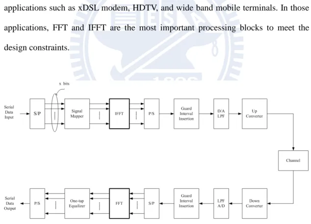
Fast Fourier Transform (FFT) and Inverse Fast Fourier Transform (IFFT) are widely used algorithms for calculating the Discrete Fourier Transform (DFT) and Inverse Discrete Fourier Transform (IDFT) because of the low computation complexity. FFT processor is an important block in communication system and signal processing system. For example, as shown in Figure 1, Orthogonal Frequency Division Multiplexing (OFDM) system is widely used in many communication applications such as xDSL modem, HDTV, and wide band mobile terminals. In those applications, FFT and IFFT are the most important processing blocks to meet the design constraints.

(11)

An automatic FFT generator can not only improve productivity but also shorten time-to-market. To support user customization, the automatic FFT generator provides some parameters to customize for the design constraints, such as the FFT transform sizes, I/O data ordering, data bitwidth, and the various architectures. In this thesis, we mainly focus on the trade-off between throughput and area of the FFT architectures.

Since the FFT algorithm was proposed by Cooley and Turkey in 1965 [1], many similar algorithms have been proposed to reduce the computation complexity of FFT. As the technology progress and algorithm improvement, FFT is widely used in Digital Signal Processing (DSP) applications. According to different algorithms, many kinds of FFT architectures have been proposed. Generally, there are two kinds of popular FFT architectures. One is memory-based architecture and the other is pipelined-based architecture. A single processing elements (PE) is used in memory-based architecture. It can be easily extended to other FFT transform sizes, so the memory-based architectures are usually used for low hardware cost and low throughput designs. Pipeline-based architectures have features such as regularity, simplicity, and high throughput rate. In this thesis, we only focus on pipelined-based architectures.

Several pipeline-based FFT architectures are proposed, such as the Radix-2 Multi-path Delay Commutator (R2MDC) [2], Radix-4 Multi-path Delay Commutator (R4MDC) [2], Radix-2 Single-path Delay Feedback (R2SDF) [3], Radix-4 Single-path Delay Feedback (R4SDF) [4], Radix-22 Single-path Delay

(12)

fewer multipliers, adders and memory size than the R4MDC; however, the R4MDC can provide higher throughput. The R22SDF has the same multiplier complex as R4SDF, but retains the butterfly structure of radix-2 algorithm. The R22MDC uses the same algorithm as the R22SDF, and the R22MDC has higher throughput. As a result, in this work, our proposed FFT generator is based on the R22MDC and the R2MDC architectures.

The rest of this thesis is organized as follows. In Chapter 2, a brief review of FFT algorithms, architectures, and automatic FFT generation is made. In Chapter 3, a detailed introduction of our approach of automatic FFT generation is made. The experimental result is presented in Chapter 4. Finally, the conclusions and the future works are given in Chapter 5.

(13)

Chapter 2 Preliminary

2.1 FFT Algorithms

2.1.1 Radix-2 DIF Algorithm

An FFT computes the DFT and produces exactly the same result as evaluating the DFT definition directly; the only difference is that an FFT is much faster.

The formulation of Length N DFT is define as

1 0 ( ) = ( ) − =

∑

N nk N n

X k x n W , k=0, 1,…,N-1 (2.1) where the coefficient W_Nnkis called twiddle factor, and is defined as

2 2 2 cos( ) sin( ) π _π _π − = j nk = − nk N N nk nk W e j N N . X (k)

is in frequency domain, and x[n] is in time domain. Radix-2 Decimation-In-Frequency

(DIF) Algorithm divided the frequency sequence X (k) into even-numbered frequency

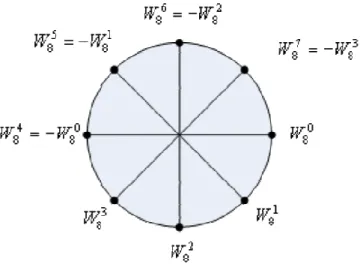
samples and odd-numbered frequency samples. Three characteristics of twiddle factor

are shown below and are illustrated in Figure 2 and Figure 3.

1. 2 2 1 π π − − = j nN = = nN _N j n N W e e 2.W_Nnk N+ 2 = −W_Nnk 3.W_N(n N k+ ) =W_Nnk

(14)

Figure 2 Characteristic 2 of twiddle factor

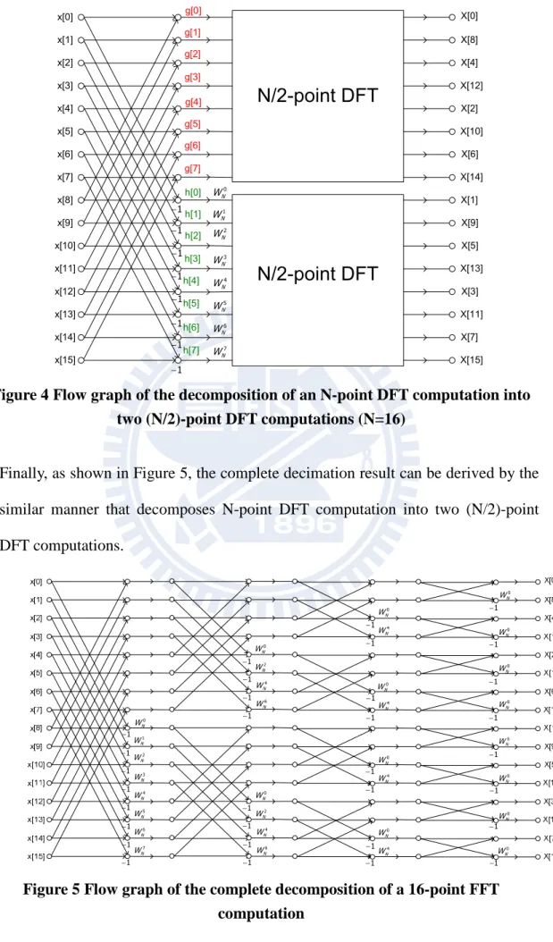
− + N n nr N N n N x n x n QW W 2 ( [ ] [ ] ) 2   =  − +    n N N N DFT x n x n W (2.3)

From the equation (2.2) and (2.3), with [ ] [ ] [ ] 2 = + + N g n x n x n and [ ] [ ] [ ] 2 = − +N

h n x n x n , it can be seen that the original N-points FFT operation has

been divided into two 2

N

(16)

x[0] x[1] x[2] x[3] x[4] x[5] x[6] x[7] x[8] x[9] x[15] x[14] x[13] x[12] x[11] x[10]

N/2-point DFT

X[0] X[8] X[4] X[12] X[2] X[10] X[6] X[14] X[1] X[9] X[5] X[13] X[3] X[11] X[7] X[15] h[0] h[1] h[2] h[3] g[0] g[1] g[2] g[3] h[4] h[5] h[6] h[7] g[4] g[5] g[6] g[7] 0 N W 1 N W 2 N W 3 N W 4 N W 5 N W 6 N W 7 N W 1 − 1 − 1 − 1 − 1 − 1 − 1 − 1 −

Figure 4 Flow graph of the decomposition of an N-point DFT computation into two (N/2)-point DFT computations (N=16)

Finally, as shown in Figure 5, the complete decimation result can be derived by the similar manner that decomposes N-point DFT computation into two (N/2)-point DFT computations. 1 N W 2 N W 3 N W 4 N W 5 N W 6 N W 7 N W 0 N W 0 N W 2 N W 4 N W 6 N W 0 N W 2 N W 4 N W 6 N W 0 N W 4 N W 0 N W 4 N W 0 N W 4 N W 0 N W 4 N W 0 N W 0 N W 0 N W 0 N W 0 N W 0 N W 0 N W 0 N W 1 − 1 − 1 − 1 − 1 − 1 − 1 − 1 − 1 − 1 − 1 − 1 − 1 − 1 − 1 − 1 − 1 − 1 − 1 − 1 − 1 − 1 − 1 − 1 − 1 − 1 − 1 − 1 − 1 − 1 − 1 − 1 −

(17)

The addition and the subtraction operation are called the butterfly operation, as show in Figure 6. [ ] x n [ ] 2 +N x n [ ] [ ] 2 + + N x n x n [ ] [ ] 2 − + N x n x n

Figure 6 Butterfly graph of Radix-2 DIF FFT

2.1.2 Radix-4 DIF Algorithm

Similar to radix-2 DIF algorithm, in the radix-4 DIF algorithm, the frequency

sequence X (k) is divided intoX(4 )k ,X(4k+1),X(4k+2), X(4k+3) frequency samples as derived below.

[ ] x n [ ] 4 +N x n [ ] 2 +N x n 3 [ ] 4 + N x n 0n N W 1n N W 2n N W 3n N W (4 ) X k (4 +1) X k (4 +2) X k (4 +3) X k

Figure 7 Butterfly graph of Radix-4 DIF FFT

2.1.3 Radix-2

2

Algorithm

Radix-4 algorithm has the lower multiplicative complexity than radix-2

(19)

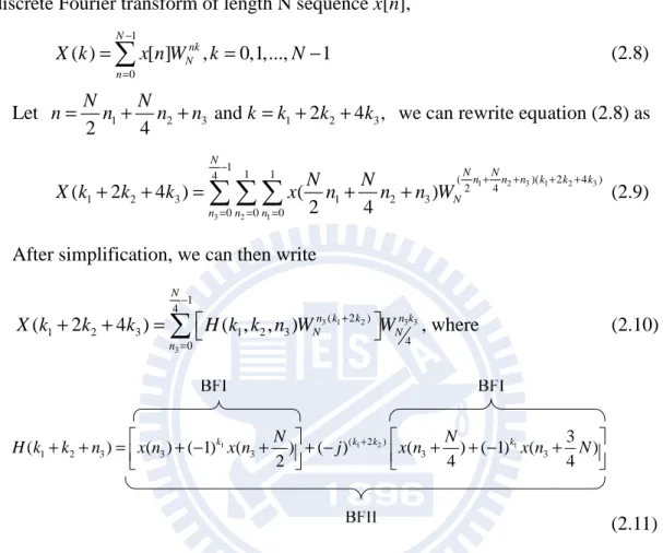
complex than that of radix-2 algorithm. Combining the advantages of radix-2 and radix-4 algorithm, Radix-22 algorithm [5] has the same multiplicative complexity as radix-4 algorithm, but retains the butterfly structure of radix-2 algorithm. For a discrete Fourier transform of length N sequence x[n],

1 0 ( ) [ ] , 0,1,..., 1 − = =

∑

N nk = − N n X k x n W k N (2.8) Let ₁ ₂ ₃ and ₁ 2 ₂ 4 ,₃ 2 4 = N +N + = + +

n n n n k k k k we can rewrite equation (2.8) as

1 2 3 1 2 3 3 2 1 1 1 1 4 ₍ ₎₍ ₂ ₄ ₎ 2 4 1 2 3 1 2 3 0 0 0 ( 2 4 ) ( ) 2 4 − + + + + = = = + + =

_{∑ ∑ ∑}

+ + N N N n n n k k k N n n n N N X k k k x n n n W (2.9)

After simplification, we can then write

3 1 2 3 3 3 1 4 ( 2 ) 1 2 3 1 2 3 4 0 ( 2 4 ) ( , , ) − + =   + + =

∑

_ _ N n k k n k N N n X k k k H k k n W W , where (2.10) 1 (1 22) 1 1 2 3 3 3 3 3 3 ( ) ( ) ( 1) ( ) ( ) ( ) ( 1) ( ) 2 4 4 +     + + =_ + − + _+ − _ + + − + _     k N k k N k H k k n x n x n j x n x n N (2.11)

From equation (2.10) and (2.11), we can find that the original N-points FFT

operation has been partitioned into four 4

N

-points FFT operations as shown in

Figure 8. After proceeding in a manner similar to the technique, a complete

decimation result can be derived as shown in Figure 9.

(20)

x[0] x[1] x[2] x[3] x[4] x[5] x[6] x[7] x[8] x[9] x[15] x[14] x[13] x[12] x[11] x[10] 4 N W 6 N W 2 N W 1 − 1 − 1 − 1 − 1 − 1 − 1 − 1 − 1 − 1 − 1 − 1 − 1 − 1 − 1 − 1 − -j -j -j -j 3 N W 3 N W 1 N W 2 N W 9 N W 6 N W N/4 DFT (k1=0,k2=0) N/4 DFT (k1=0,k2=1) N/4 DFT (k1=1,k2=0) N/4 DFT (k1=1,k2=1) X[0] X[8] X[4] X[12] X[2] X[10] X[6] X[14] X[1] X[9] X[5] X[13] X[3] X[11] X[7] X[15]

Figure 8 Flow graph of the decomposition of an N-point DFT computation into four (N/4)-point DFT computations (N=16) with radix-22 algorithm

1 − 1 − 1 − 1 − 1 − 1 − 1 − 1 − 1 − 1 − 1 − 1 − 1 − 1 − 1 − 1 − 1 − 1 − 1 − 1 − 1 − 1 − 1 − 1 − 1 − 1 − 1 − 1 − 1 − 1 − 1 − 1 − 4 N W 6 N W 2 N W 3 N W 3 N W 1 N W 2 N W 9 N W 6 N W 0 N W 0 N W 0 N W 0 N W 0 N W 0 N W 0 N W 0 N W 0 N W 0 N W 0 N W

Figure 9 Flow graph of the complete decomposition of a 16-point FFT computation with radix-22 algorithm

(21)

2.1.4 Split-Radix Algorithm

The split-radix algorithm can further reduce the complexity of the FFT algorithm. It has fewer multiplications and additions than radix-2 and radix-4 algorithm, but radix-2 and radix-4 algorithm are more regular than split-radix algorithm. The most popular split-radix algorithm including radix-2/4 and radix-2/8 were proposed in [8].

2.2 FFT Architectures

Generally, there are two kinds of popular FFT architectures to implement FFT algorithms. One is memory-based architectures and the other is pipeline-based architectures. Memory-based architectures are suitable for low throughput and low hardware cost designs; however, pipeline-based architectures are usually regular and suitable for high throughput and high hardware cost designs. In this thesis, we focus on pipeline-based FFT architectures. The details of pipeline-based architectures are presented in the following subsections.

2.2.1 Pipeline Architectures

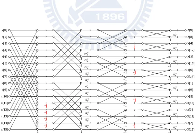
Pipeline-based architectures can be further divided into two kinds of architectures depend on the design of register. One is Single-path Delay Feedback (SDF) architecture, and the other one is Multi-path Delay Commutator (MDC) architecture. SDF architecture has higher hardware usage and lower hardware cost; however, MDC architecture has higher throughput than SDF architecture. We

(22)

next stage when doing addition operation, and storing the output into the shift register when doing subtraction operation. In each cycle, only one output passes through the multiplier.

Figure 10 R2SDF architecture (N=16)

The Radix-4 SDF (R4SDF) architecture [4] is shown in Figure 11. Similar to the R2SDF architecture, radix-4 butterfly store three of outputs into shift registers, and only one output passes through the multiplier in each cycle.

The Radix-22 SDF (R22SDF) [5] architecture is similar to the R2SDF architecture and reduces the number of multipliers. R22SDF uses two types of butterflies, one is the same as that in R2SDF architecture and the other contains also some logic to implement the multiplication of twiddle factor of –j, as shown in Figure 12.

(23)

The Radix-2 MDC (R2MDC) architecture [2] is straightforward. The inputs are separated into two streams by the control of switches, and then go to butterflies in parallel, as shown in Figure 13.

(24)

Figure 14 R4MDC Architecture (N=16)

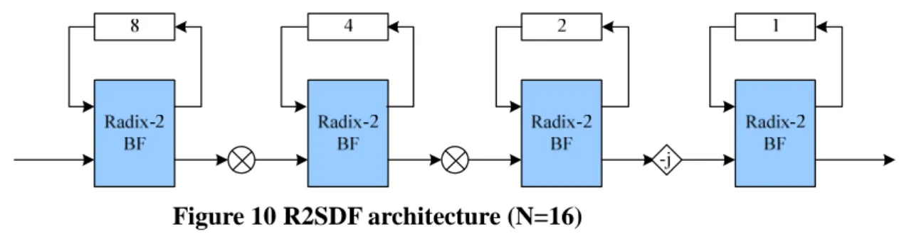
The Radix-22 MDC (R22MDC) architecture [6] is the MDC type architecture of Radix-22 algorithm. In the flow graph of the complete decomposition of an N-point FFT computation with radix-22 algorithm, the even-numbered stages multiple twiddle factors not only the subtraction output but the addition output, so the R22MDC architecture needs two complex multipliers in even-numbered stages, as shown in Figure 15.

Figure 15 R22MDC architecture (N=16)

2.2.2 Memory-Based Architectures

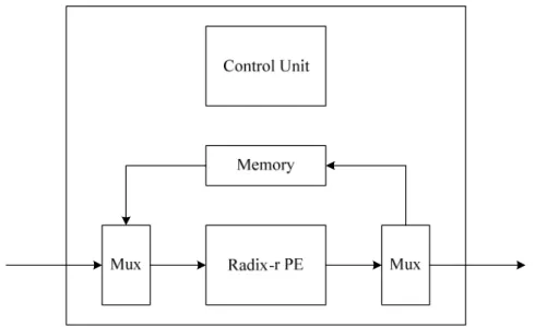
The memory-based architecture is another widely used FFT architecture. It only uses one radix-r processing element to compute all butterflies in signal flow graph. The basic components of memory-based architecture are shown in Figure 16. In Figure 16, the multiplexers are used to control the input and output data, and because of only single PE, the controller of memory-based architecture is very complex. Because of low hardware cost and low power properties, memory-based architecture is suitable for modern communication system.

(25)

Figure 16 A memory-based architecture example

2.3 Automatic FFT Generation

An automatic FFT Generator can improve productivity and shorten time-to-market. A customized FFT generator with parameterized options can be tailored for application-specific trade-off in performance. Three papers about parameterized FFT Generator have been published [11]. In the following, we briefly introduce the techniques in [11] and [13].

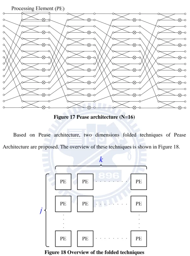
In [11] and [13], they make the trade-off between area and throughput based on Pease architecture. After replacing twiddle factors with complex multipliers and exchanging the positions of butterflies, the16-points Pease architecture can be derived from the flow graph of the complete decomposition of the 16-point FFT computation with radix-2 algorithm, as shown in Figure 17. From Figure 17, we can derive the

(26)

Figure 17 Pease architecture (N=16)

Based on Pease architecture, two dimensions folded techniques of Pease Architecture are proposed. The overview of these techniques is shown in Figure 18.

Figure 18 Overview of the folded techniques

As shown in Figure 18, parameter j indicates the number of PEs per stage, and j needs to be one of the factors of

2

N

; parameter k indicates the number of stages,

(27)

be derived by choosing parameter j and k. For N=16, all possible choices of (j, k) are (1,1), (1,2), (1,4), (2,1), (2,2), (2,4), (4,1), (4,2), (4,4), (8,1), (8,2) and (8,4), Figure 19 shows some overviews of choices of N=16.

PE PE PE PE PE PE PE PE PE PE PE PE PE PE PE PE PE PE PE PE PE PE PE PE PE PE PE PE PE PE PE PE

(8,4)

Figure 19 Overview of the folded techniques example for N=16

We further introduce the folded techniques. From Figure 17, we can straightforward fold the Pease architecture fully in horizontal direction by using a multiplexer and inserting registers at the outputs of PEs. A vector iterates over the

feedback log₂ N times to compute the FFT. Figure 20 shows a full

(28)

Figure 20 A full horizontally-folded Pease FFT for N=16

Starting from the full horizontally-folded architecture, the

2

N

PEs can be further folded in vertical direction to achieve different degrees of parallelism and therefore different throughputs. A full horizontally-folded and vertically-folded Pease FFT for N=16 is shown in Figure 21.

Figure 21 A full horizontally-folded and vertically-folded Pease FFT for N=16

The main problem of vertically-folded is how to buffer and reorder the data.

Without vertical folding, data buffering is just inserting registers at the PEs’ outputs,

and data reordering is a simple wiring. Takala et al. [14] describes a vertically-folded

2j j

(29)

implementation of general stride permutation. Figure 22 is the overview of stride permutation. The stride permutation can be decomposed into two structures. One is interconnection permutation 2j ( n : a mod −1 (0≤ < −1), 1a −1)

j m

L L i mi n i n n - n ,

an example of L4₂ is shown in Figure 23, and the other is Dm block, as shown in

Figure 24. The Dm block contains two m-entry synchronous FIFOs and a switch that

allows the two either to pass-through for m cycles or to criss-cross for m cycles. Comparison of hardware cost and throughput is listed in Table 1.

2j j

L

Figure 22 An overview of stride permutation

Figure 23 An example of 4 2

(30)

Following Figures are some examples for N=16. Figure 25 An example of (j,k)=(1,1) Figure 26 An example of (j,k)=(2,1) Figure 27 An example of (j,k)=(2,2) Figure 28 An example of (j,k)=(4,1)

Table 1 Comparison of hardware cost and throughput

FFT Length multipliers adders registers throughput

N jk 2jk N 2 log jk N N D2 D2 4 2 L 4 2 L L42 D1 8 4 L

(31)

Chapter 3 Proposed Approach

3.1 Motivation

An exhaustive search approach is proposed to find all possible FFT architectures and then generate a set of acceptable FFT architecture according to the design constraints. However, from Table 1, we can find that all the possible solutions have the same number of multipliers, number of adders and number of registers usage under the throughput constraint.

Pease architecture bases on the radix-2 algorithm. Observing the raidx-2 flow graph in Figure 5, each butterfly is followed by a multiplication operation at the output of subtraction operation. Therefore, Pease architecture is a very regular architecture. However, the radix-2 algorithm contains many trivial multiplications which do not need multipliers to calculate. For example, multiplication of –j involves only real-imaginary swapping and sign inversion, as shown in Figure 29.

(32)

The radix-22 algorithm considers the multiplication of –j and merges the multiplication of –j into odd-numbered columns, as shown in Figure 9. And the architecture of radix-22 algorithm contains two kinds of butterflies, BFI and BFII. From the view of architecture, the radix-22 algorithm is more irregular than the radix-2 algorithm.

The R22MDC [6] is a pipeline architecture that implements the radix-22 algorithm with throughput 2

N , so R2

2

MDC architecture is more irregular than Pease

architecture. In the following subsections, we introduce how we make the trade-off

between hardware and throughout based on R22MDC and R2MDC architecture.

3.2 R2

2

MDC Vertical Expansion Architecture

The R22MDC architecture for N=16 is shown in Figure 30. Because of the property of this architecture, the throughput of R22MDC architecture is 2

N , and the

throughput is1

8 for N=16.

Figure 30 R22MDC architecture with throughput =1

8, N=16

Now, if we want to increase the throughput, a straightforward approach is to

parallelize the original architecture. However, parallelizing the R22MDC architecture is not an easy task because of the complexity of the controller and data dependence. It

may not be a hard task by using two R22MDC architectures to parallelize, but the difficulty will increase if we want to increase the degree of parallelism. An automatic

(33)

3.2.1 Interconnection Permutation Matrix

We first introduce the interconnection permutation matrix, In. The

interconnection permutation matrix represents wiring relationship between different R22MDC architectures. The rules of In are shown in following.

In: , ( mod 2) ( 1) 2 2 < n a + × N − i i i i , ( mod 2) ( 1) ( 1) 2 2 2 ≥n a + × N − − N − i i i i

Following the rules, two examples are shown in Figure 31

0

1

2

3

0

1

2

3 I

4

0

1

2

3

0

1

2

3 I

8

4

5

6

7

4

5

6

7

(34)

3.2.2 The Proposed R2

2

MDC Vertical Expansion Architecture

A general form of R22MDC vertical expansion architecture is shown in Figure 32. Parameter N indicates the FFT transform size, where =2 ,m =1, 2,3...

N m .Parameter t

indicates the degree of parallelism, wheret=1, 2, 4..., 2m−1. The number of registers of each original R22MDC architecture decreases as the degree of parallelism increases, and the number of interconnection permutation matrix also increases. With the interconnection permutation matrix, data dependence would be kept. From Figure 32, we can derive the number of multipliers is t(2 log_ ₄N_- 2), the number of adders is

2

2 logt N , the number of registers is N −2t and the throughput is 2t

N . 16 N t 8 N t 4 N t 1 16 N t 8 N t 4 N t 1

Figure 32 General form of R22MDC vertical expansion architecture

Figure 33 shows the case when t =1, the original R22MDC architecture, the number of multiplier is 2, the number of adders is 8, the number of registers of datapath is 14, and the throughput is1

8.

Figure 33 Example of R22MDC vertical expansion architecture for t=1

(35)

of adders is 16, the number of registers of datapath is 12, and the throughput is1

4.

Figure 35 shows the case when t =4, the number of multipliers is 8, the number

of adders is 32, the number of registers of datapath is 8, and the throughput is1 2.

Figure 36 shows the case when t =8, namely, a fully parallelized R22MDC vertical expansion architecture, the number of multipliers is 16, the number of adders

is 64, the number of registers of datapath is 0, and the throughput is1 2.

(36)

3.2.3 The Limitation of R2

2

MDC Compression

As mentioned in previous work, they provide two dimensions folded techniques for trade-off between area cost and throughput. However, horizontal compression approach of R22MDC architecture is not suitable. Because of the irregularity of the R22MDC architecture, advantages would be eliminated when compressing the R22MDC architecture, as illustrated in Figure 37. Figure 37 is an example that shows three architectures for the same throughput1

8. Figure 37(a) shows the R2

2

MDC

architecture with t = 1, the number of adders is 8, and the number of multipliers is 2,

(37)

37(c) shows the horizontal compression R22MDC architecture after paralleling with t = 4, the number of adders is 8, and the number of multipliers is 8. We can find that hardware requirement of horizontal compression architectures is worse than the R22MDC architecture without horizontal compression under the same throughput constraint.

(a)

(b) (c)

Figure 37 Hardware usage comparison based on R22MDC architecture for N=16, throughput=1

8.

Therefore, we choose another base architecture if horizontal compression is

necessary. The R2MDC architecture is more suitable than R22MDC architecture for horizontal compression, as illustrates in Figure 38. In Figure 38 (a), the number of

(38)

multipliers, we do not use this architecture because of the choice of R22MDC architecture.

(a)

(b) (c)

Figure 38 Hardware usage comparison based on R2MDC architecture for N=16, throughput=1

8.

(39)

3.3 R2MDC Horizontal Compression Architecture

In section 3.2, we introduced the R22MDC vertical expansion architecture which can increase the throughput with increasing the area cost, and as mentioned in section 3.2.3, R2MDC architecture is suitable for horizontal compression. In this section, we illustrate how to compress the R2MDC architecture horizontally.

For an R2MDC architecture with transform size N, we can divide the N-points R2MDC architecture into log₂N stages. In our approach, we can provide m kinds of horizontal architectures, where m is the number of the factors of log2N, and the

factors f indicates the compression degree. We define t = 1

f for horizontal

compression. For example, assume N=16, then the factors of 4 are 1, 2, 4. We have three kinds of architectures for N=16, and 1, 2, 4 indicate different degrees of compression as illustrate in Figure 39. In Figure 39(a), t = 1

f =1, the compression

degree is 1 means no horizon compression occurs, the architecture of t = 1 is the same as the R2MDC architecture. In Figure 39(b), the compression degree is 1

2 which

means compressing the number of stages of R2MDC architecture to half of original architecture, so, the number of stages in decreases to 2, and the data need to iterate

(40)

(a)

(b)

(c)

Figure 39 Examples of horizontal compression for N=16, (a) t=1(b) t =1

2(c) t = 1 4

(41)

3.4 Summary

In section 3, we proposed two directional trades-off approaches based on R22MDC architecture and R2MDC architecture. In vertical direction, we provide an expansion approach for R22MDC architecture to increase the throughput, and in horizontal direction, we provide a compression approach for R2MDC architecture to decrease the throughput. Under the throughput constraint, our approach can provide only one exact solution; however, as mentioned in section 2, they search the desired solution exhaustively. Table 2 lists the hardware and throughput comparison between our approach and previous work. Table 3 lists the hardware and throughput comparison with the same throughput by replacing jkwith tlog2N.

Table 2 Hardware Requirement Comparison

FFT length (N) multipliers adders registers throughput

Pease jk 2jk N 2 2 log jk N N R22MDC_P t(2 log 4N−2) 2 logt 2 N N-2t 2t N R2MDC_F tlog2N 2 logt 2 N N 2t N

Table 3 Hardware Requirement Comparison with the same throughput

FFT length (N) multipliers adders registers throughput

Pease tlog2N 2 logt 2N N

2t

N

R22MDC_P t(2 log 4 N−2) 2 logt 2N N-2t

2t

(42)

Chapter 4 Experiments

4.1 Experimental Environment

We implement two kinds of FFT architectures, including R22MDC vertical expansion architecture and R2MDC horizontal architecture. Each PE stage of FFT architecture is piped. The complex adder contains two real adders and the complex multiplier contains four real multipliers and two real adders, as shown in Figure 40. For each complex multiplier, we design a ROM which contains all the possible twiddle factor values for this complex multiplier.

×

+

Figure 40 Complex Multiplier

Logic gate model includes adder, multiplier, and multiplexer. We use UMC 0.18um cell library and Synopsys DesignWare [15] to synthesis under 100MHz clock rate. The platform is built in an Intel dual Pentium Xeon at 2.5GHz with 32GB of main memory, running Linux.

We use Matlab [16] to generate random inputs, and calculate the SQNR to guarantee the correctness of the generated FFT architecture. Our simulation results of SQNR are between 80 (db) and 90 (db).

(43)

4.2 Experimental Results

Figure 41 shows the relation between throughput and area for N=256, where area indicates the number of gate counts. For Pease, three architectures are generated, from left to right, the parameters are j=1, j=2, and j=4respectively. For all architectures, we assume k=1. For R2MDC, three architectures are generated, from left to right, the parameters

are 1 8 = t , 1 4 = t , and 1 2 =

t respectively. We can find that the area of Pease is almost the

same as the area of R2MDC under the same throughput. From Table 3, we can find that the

hardware requirement is also the same under the same throughput. Figure 42 shows the

relation between throughput and area for N=1024. For Pease, three architectures are

generated, from left to right, the parameters are j=1, j=2, and j=4 respectively. For all architectures, we also assume k=1. For R2MDC, three architectures are generated, from

left to right, the parameters are 1 10 = t , 1 5 = t , and 1 2 =

t respectively. The trend is almost

the same as N=256 in Figure 41.

FFT Length N=256 FFT Length N=256FFT Length N=256 FFT Length N=256 20 40 60 80 100 120 140 K K K K A re a ( g a te c o u n ts ) A re a ( g a te c o u n ts ) A re a ( g a te c o u n ts ) A re a ( g a te c o u n ts ) Pease R2MDC

(44)

FFT Length N=1024 FFT Length N=1024 FFT Length N=1024 FFT Length N=1024 320 330 340 350 360 370 380 0 0.0002 0.0004 0.0006 0.0008 0.001 0.0012 K KK K Throughput Throughput Throughput Throughput A re a A re a A re a A re a _Pease R2MDC

Figure 42 Relation between throughput and area for Pease and R2MDC, N=1024

Figure 43 shows the relation between throughput and area for N=256. For Pease, five architectures are generated, from left to right, the parameters are j=8, j=16,…, and j=128 respectively. For R22MDC, six architectures are generated, from left to right, the parameters are t=1, t=2,…, and t=32 respectively. We can find that the area of Pease is greatly larger than the area of R22MDC vertical expansion architectures under the same throughput because of the great number of multipliers

usage of Pease. It can be also seen in Table 3. Figure 44 shows the relation between

throughput and area for N=1024. For Pease, five architectures are generated, from left

to right, the parameters are j=8, j=16 ,…, and j=128 respectively. For R22MDC, five architectures are generated, from left to right, the parameters are t=1,

2

=

t ,…, and t =16 respectively. We can find that the area of Pease is still greatly larger than the area of R22MDC vertical expansion architectures under the same throughput.

(45)

FFT Length N=256 FFT Length N=256FFT Length N=256 FFT Length N=256 0 500 1000 1500 2000 2500 0 0.05 0.1 0.15 0.2 0.25 0.3 K K K K Throughput Throughput Throughput Throughput A re a ( g a te c o u n ts ) A re a ( g a te c o u n ts ) A re a ( g a te c o u n ts ) A re a ( g a te c o u n ts ) Pease R22MDC Figure 43 Relation between throughput and area for Pease and R22MDC, N=256

FFT Len gth N=10 24 FFT Len gth N=10 24 FFT Len gth N=10 24 FFT Len gth N=10 24 0 500 1000 1500 2000 2500 0 0.005 0.01 0.015 0.02 0.025 0.03 0.035 K K K K Throug hp ut Throug hp utThroug hp ut Throug hp ut A re a ( g a te c o u n ts ) A re a ( g a te c o u n ts ) A re a ( g a te c o u n ts ) A re a ( g a te c o u n ts ) Pease R22MDC

Figure 44 Relation between throughput and area for Pease and R22MDC, N=1024

(46)

FFT Length N=256 FFT Length N=256 FFT Length N=256 FFT Length N=256 0 500 1000 1500 2000 2500 0 0.05 0.1 0.15 0.2 0.25 0.3 K Throughput Throughput Throughput Throughput A re a (g at e c o u n ts ) A re a (g at e c o u n ts ) A re a (g at e c o u n ts ) A re a (g at e c o u n ts ) Pease R2MDC/R22MDC

Figure 45 Relation between throughput and area for Pease and R2MDC/R22MDC, N=256

0 500 1000 1500 2000 2500 0 0.005 0.01 0.015 0.02 0.025 0.03 0.035 A re a (g at e co u nt s) A re a (g at e co u nt s) A re a (g at e co u nt s) A re a (g at e co u nt s) K Throughput Throughput Throughput Throughput FFT Length N=1024 FFT Length N=1024FFT Length N=1024 FFT Length N=1024 Pease R2MDC/R22MDC

Figure 46 Relation between throughput and area for Pease and R2MDC/R22MDC, N=1024

Compared with the Pease architecture, for the length of 256 and 1024 cases, the generated FFT processor saves about 30.8% area under throughput constraints, as shown in Table 4.

(47)

Table 4 Area comparison

FFT Length (N)

Pease R22MDC Area Reduction

Percentage (%)

Throughput Area Throughput Area

256 0.0078 190524 0.0078 128033 32.8 0.0156 307040 0.0156 202469 34.06 0.0313 533357 0.0313 350469 34.29 0.0625 1044244 0.0625 641511 38.57 1024 0.0016 434154 0.002 313669 27.75 0.0031 565576 0.0039 417760 26.14 0.0063 825269 0.0078 623772 24.42 0.0125 1314636 0.0156 1029338 21.70

(48)

Chapter 5 Conclusions and Future Work

The FFT processor is an important computing block in communication and signal processing systems. To improve productivity and shorten time-to-market, an automatic FFT generator can be used to design a specified FFT processor. In this thesis, we propose a parameterizable FFT generator with two approaches to make good design trade-off between throughput and area under the design constraints. First, the vertical expansion approach parallels the datapath to increase the throughput. Second, the horizontal compression approach folds the datapath to reduce the hardware usage. Besides, only the best FFT architecture is generated under the user-specified throughput constraint to reduce the computation time in our proposed FFT generator. Compared with the Pease architecture, for the length of 256 and 1024 cases, the generated FFT processor saves about 30.8% area under throughput constraints.

Various FFT architectures are proposed in literature. It can be implemented into our proposed FFT generator. In the future, more FFT algorithms such as the R23MDC FFT algorithm, mixed-radix FFT [17] algorithm will be considered to enlarge the search space. Besides, the bitwidth optimization techniques proposed in [18] will also be considered.

(49)

Reference

[1] J. W. Cooley and J. W. Turkey, “An Algorithm for Machine Computation of Complex Fourier Series,” Math. Computation, Vol. 19, pp. 297-301, April 1965.

[2] L. R. Rabiner and B. Gold. Theory and Application of Digital Signal Processing. Prentice-Hall, Inc., 1975.

[3] E. H. Wold and A. M. Despain, “Pipeline and Parallel-Pipeline FFT Processors for VLSI Implementation,” IEEE Trans. Computers, vol. 33, no. 5, pp. 414-426, May 1984.

[4] A.M. Despain. “Fourier Transform Computer using CORDIC Iterations,” IEEE Trans. Comput., C-23(10):993-1001, Oct.1974.

[5] S. He and M. Torkelson, “A New Approach to Pipeline FFT Processor,” in Proc. 10th Int’l Parallel Processing Symp. (IPPS ’96), pp.766-770, 1996.

[6] R. Storn. “Radix-2 FFT-pipeline Architecture with Reduced Noise-to-signal Ratio,” IEE Proceedings- Vision, Image and Signal Processing, 141:81-86, 1994.

[7] S. He and M. Torkelson, "Designing Pipeline FFT Processor for OFDM (de)Modulation", International Symposium on Signals, Systems, and Electronics, pp. 257- 262, Oct. 1998.

[8] P. Duhamel, H. Hollmann, “Split Radix FFT Algorithm,” Electronics Letters, vol. 20, pp.14-16, January 1984.

[9] P. Duhamel, and H. Hollmann, “Split Radix FFT Algorithm,” Electronics Letters, vol. 20, pp. 14-16, Jan. 5, 1984.

(50)

[11] G. Nordin, P. A. Milder, J. C. Hoe, and M. Püschel, “Automatic Generation of Customized Discrete Fourier Transform IPs,” In Proc. of ACM/IEEE Design Automation Conf., pp. 471-474, 2005.

[12] P. A. Milder, M. Ahmad, J.C. Hoe, and M. Püschel, “Fast and Accurate Resource Estimation of Automatically Generated Custom DFT IP Cores,” In Proc. of the ACM/SIGDA International Symposium on Field Programmable Gate Arrays, pp. 211-220 2006.

[13] P. A. Milder, F. Franchetti, J. C. Hoe, and M. Püschel, “Formal Datapath Representation and Manipulation for Implementing DSP Transforms,”In Proc. of ACM/IEEE Design Automation Conf., pp. 385-390, 2008.

[14] J. Takala, T.Jarvinen, P. Salmela, and D. Akopial. Multi-port Interconnection Networks for Radix-r Algorithms. In Proc. IEEE International Conference Acoustics, Speech, Signal Processing, pp. 1177-1180, 2001.

[15] Synopsys DesignWare[Online], Available: http://www.synopsys.com .

[16] Matlab [Online], Available: http://www.mathworks.com .

[17] R.C. Singleton, “An Algorithm for Computing the Mixed Radix Fast Fourier Transform,” IEEE Trans. on AudioElectroacoust., vol. 1, no. 2, pp. 93-103, June 1969.

[18] C.Y. Wang, C.B. Kuo, and J.Y. Jou, “ Hybrid Word-Length Optimization Methods of Pipelined FFT Processors”, IEEE Trans. Computers, vol. 56, no. 8, pp. 1105- 1118, Aug. 2007.

[19] P.D. Welch, “A Fixed-Point Fast Fourier Transform Error Analysis,” IEEE Trans. Audio Electroacoustics, vol. 17, pp. 151-157, June 1969.

[20] A. Pomerleau, H.L. Buijs, and M. Fournier, “A Two-Pass Fixed Point Fast Fourier Transform Error Analysis,” IEEE Trans. Acoustics, Speech, and Signal Processing, vol. 25, pp. 582-585, Dec. 1977.

高效能且低成本之可參數化快速傅利葉轉換硬體產生器

國立交通大學

國立交通大學

國立交通大學

國立交通大學

電子工程學系

電子工程學系

電子工程學系

電子工程學系

電子研究所

電子研究所

電子研究所

電子研究所

碩

碩

碩

碩

士

士

士

士

論

論

論

論

文

文

文

文

高效能且低成本之可參數化快速傅利葉轉

換硬體產生器

A Parameterizable Generator for High-Performance and

Low-Cost FFT Cores

研 究 生：王毓翔

高效能且低成本之可參數化快速傅利葉轉換

高效能且低成本之可參數化快速傅利葉轉換

高效能且低成本之可參數化快速傅利葉轉換

高效能且低成本之可參數化快速傅利葉轉換

硬體產生器

硬體產生器

硬體產生器

硬體產生器

A Parameterizable Generator for High-Performance

and Low-Cost FFT Cores

研究生：王毓翔 Student: Yu-Hsiang Wang

指導教授：周景揚 教授 Advisors: Jing-Yang Jou

黃俊達 博士 Juinn-Dar Huang

國立交通大學

電子工程學系 電子研究所

碩士論文

高效能且低成本之可參數化快速傅利葉轉換

高效能且低成本之可參數化快速傅利葉轉換

高效能且低成本之可參數化快速傅利葉轉換

高效能且低成本之可參數化快速傅利葉轉換

硬體產生器

硬體產生器

硬體產生器

硬體產生器

摘要

摘要

摘要

摘要

A Parameterizable Generator for

High-Performance and Low-Cost FFT Cores

Abstract

Acknowledgment

Content

List of Figures

List of Tables

Chapter 1

Introduction

Chapter 2

Preliminary

2.1 FFT Algorithms

2.1.1 Radix-2 DIF Algorithm

∑

∑

∑

∑

∑

研究生：王毓翔

指導教授：周景揚教授 Advisors: Jing-Yang Jou

黃俊達博士 Juinn-Dar Huang

電子工程學系電子研究所

_∑

_∑

_∑

_∑

_∑

_∑

_{∑ ∑ ∑}