國立交通大學
電子工程學系 電子研究所
博 士 論 文
針對 FIR 與 FFT 演算法於超大型積體電路
實作上之解析式面積最佳化技術
Analytical Area Optimization for VLSI
Implementations of FIR and FFT Algorithms
研 究 生:林步青
指導教授:周景揚 博士
黃俊達 博士
針對 FIR 與 FFT 演算法於超大型積體電路
實作上之解析式面積最佳化技術
Analytical Area Optimization for VLSI
Implementations of FIR and FFT Algorithms
研究生:林步青
Student: Bu-Ching Lin
指導教授:周景揚 博士
Advisors: Jing-Yang Jou
黃俊達 博士
Juinn-Dar Huang
國立交通大學
電子工程學系 電子研究所
博士論文
A Dessertation
Submitted to Department of Electronics Engineering & Institute of Electronics College of Electrical & Computer Engineering
National Chiao Tung University in Partial Fulfillment of the Requirements
for the Degree of Doctor of Philosophy
in
Electronics Engineering & Institute of Electronics
June 2014
Hsinchu, Taiwan, Republic of China
針對 FIR 與 FFT 演算法於超大型積體電路
實作上之解析式面積最佳化技術
研究生:林步青 指導教授:周景揚博士 黃俊達博士 國立交通大學 電子工程學系及電子研究所 博士班摘要
在過去幾十年中,隨著通信系統的複雜度急劇增加,數位訊號處理演算法 被廣泛地採用,例如有限脈衝響應(FIR)濾波器和快速傅利葉轉換(FFT)。其中, 多常數乘法(MCM) 是在處理輸入資料與常數的乘法時,使用一組加法器取代 常規乘法器,其概念更是廣泛地被應用在有限脈衝響應濾波器的設計中。在過 去,雖然已有很多降低加法器用量之演算法被提出以達到面績縮小的目的,但 是,它們並未考慮每個加法器的實際位元數,而這將會導致估計的硬體成本不 夠精確。因此這篇論文中,我們提出了一個保證位元數的多個常數乘法最佳化 演算法,著重於最大限度地減少加法器的總位元數,而不是僅考慮減少加法器 總數。首先,構建基於給定係數的子表達式圖表,繼而導出一組針對最小化加 法器位元數之條件,最後使用整數線性規畫得到最佳化的結果。實驗結果顯示, 該演算法的確可以有效地減少所需的加法器位元數並且優於所有的現行技術。 此外,快速傅利葉轉換處理器在眾多以數位訊號處理為基礎的系統中是一 個核心的元件;例如,現代無線通信中的正交分頻多工(OFDM)。許多關鍵的 設計參數,如架構,位元長度,和數字格式,都必須非常仔細地考慮。在過去 的幾十年,針對不同的設計目標,已經有很多最佳化的管線式快速傅利葉轉換 架構被提出。雖然固定的管線式快速傅利葉轉換架構能在合理的硬體成本下提 供不錯的處理能力,但是,在針對需要大量處理能力的應用上,它可能仍然無 法滿足效能的需求。因此在這篇論文中,我們提出了一種可擴展的多路徑延遲 累積器式之快速傅利葉轉換架構及其相應的硬體設計產生器,在給定的處理能 力條件下,它能夠迅速地產生對應的快速傅利葉轉換核心。實驗結果顯示,此 方法所產生之快速傅利葉轉換器比現有的可折疊式多路徑延遲累積器式快速 傅利葉轉換架構,面積更小且功率效率更高。 除此之外,我們亦提出了一個快速傅利葉轉換器最佳化的設計流程。在固 定位元長度的條件下,正確的調整每一個蝴蝶級的定點表示之數值,以最大化 輸出級的信號量化雜訊比(SQNR)。所提出的流程採用機率分佈模型來模擬每 個階段的輸出信號的機率行為。由於量化和飽和運算所導致的雜訊可以靜態分 析,以了解在進行縮放決策時的影響。因此,不需耗費時間的模擬分析,我們 所提出的方法即可有效地決定每一個蝴蝶級的最適當的數字格式,從而最佳化 整個輸出級的信號量化雜訊比。此外,建議的流程能夠處理各種快速傅利葉轉 換點數、快速傅利葉轉換演算法、字元長度、以及輸入信號的機率分佈。實驗 結果顯示,我們的方法可以在 8192 點且以 2 為基數的快速傅利葉轉器處理器 中節省 3 位元的字元長度,而且不會對輸出級的信號量化雜訊比造成影響。使 用我提出的靜態尺規最佳化的技術所創建的快速傅利葉轉器處理器的信號量 化雜訊比可以近似於一個配有額外的動態尺規化方法,但不需要其額外龐大的 硬體成本。
Analytical Area Optimization for VLSI Implementations
of FFT and FIR Algorithms
Student: Bu-Ching Lin Advisor: Dr. Jing-Yang Jou Dr. Juinn-Dar Huang
Department of Electronics Engineering Institute of Electronics
National Chiao Tung University
Abstract
As the complexity of communication systems has grown dramatically in the past decades, digital signal processing algorithms are extensively used, such as finite-impulse-response filter (FIR) and fast Fourier transform (FFT). Meanwhile, the notion of multiple constant multiplication (MCM) is extensively adopted in FIR designs. A set of adders are used to replace regular multipliers for the multiplications between input data and constant filter coefficients. Though many algorithms have been proposed to reduce the total number of adders in an MCM block for area minimization, they do not consider the actual bitwidth of each adder, which may not estimate the hardware cost well enough. Therefore, we propose a bitwidth-aware MCM optimization algorithm that focuses on minimizing the total number of adder bits rather than the adder count. It first builds a subexpression graph based on the given coefficients, derives a set of constraints for adder bitwidth minimization, and
then optimally solves the problem through integer linear programming (ILP). Experimental results show that the proposed algorithm can effectively reduce the required adder bit count and outperforms the existing state-of-the-art techniques.
The FFT processor serves as one of core components in numerous DSP-based systems, such as OFDM in modern wireless communication. The key design parameters, such as architecture, wordlength, and number format, must be all considered very carefully. Many pipelined FFT architectures optimized for different objectives have been proposed in past few decades. Though a fixed pipelined FFT architecture can generally provide good throughput at reasonable hardware cost, it may still fail to meet the performance demand for throughput-hungry design cases. In this dissertation, we propose an expandable MDC-based FFT architecture as well as the corresponding hardware design generator, which is capable of automatically producing an FFT core under a given throughput constraint. The experimental results show that the proposed methodology can generate smaller and power-efficient implementations than the existing foldable MDC-based FFT architecture.
Besides, in this dissertation, we also propose an optimization flow that properly scales fixed-point numeric values at each butterfly stage to maximize the output SQNR under a fixed wordlength constraint. The proposed flow utilizes probability distribution to model the probabilistic behavior of the output signal at each stage. The computation errors due to quantization and saturation operations are statically analyzed before making scaling decisions. Therefore, without a need of time-consuming simulation, our method can efficiently determine the most appropriate number format for each stage and thus optimize the overall output SQNR. Besides, the proposed flow is capable of handling various FFT sizes, FFT algorithms, wordlengths, and input signal distributions. Experimental results indicate that the wordlength can be reduced about three bits for an 8K-point radix-2 memory-based
FFT processor without compromise in the output SQNR. Furthermore, the FFT processor created using our static scaling optimization technique can produce a comparable output quality as the one equipped with an extra dynamic number scaling unit, which requires significantly more hardware logic.
Acknowledgment
First and foremost, I would like to express my greatest appreciation to my advisors, Professor Jing-Yang Jou (周景揚) and Professor Juinn-Dar Huang (黃俊達) for their suggestions, guidance, and patience. Their wisdom, knowledge, and commitment to the highest standards inspired and motivated me.
Also, I would like to thank the involved members in the projects, Jhih-Hung Lu (呂智宏), Yu-Hsiang Wang (王毓翔), Ming-En Stone (石銘恩), Yao-Chung Hsu (許 耀中), and Yi-Fang Chen (陳奕方). Without the seamless cooperation, the projects would not be so successful. Thanks to Geeng-Wei Lee (李耿維), Cheng-Yeh Wang (王成業), Zwei-Mei Lee (李瑞梅), Chia-I Chen (陳嘉怡), Ya-Shih Huang (黃雅詩), and Wan-Yu Lee (李婉毓) for several useful discussions. A special thanks to all EDA members for the wonderful time we share together.
I would like express my sincere appreciation to Yi-Fang Huang (黃儀芳), my wife, without whom this effort would have been worth nothing. Your love support, and constant patience have taught me so much about sacrifice, discipline, and compromise. I would appreciate my family for their patient wait and my father education philosophy “no wonder sometimes incompetent people win out in imperial examinations, but does these mean that the erudite ones will be neglected?”
B
U-C
HINGL
INNational Chiao-Tung University June, 2014
Content
針對 FIR 與 FFT 演算法於超大型積體電路實作上之解析式面積最佳化技術 .... iii
摘要... iii
Analytical Area Optimization for VLSI Implementations of FFT and FIR Algorithms v Abstract ... v Acknowledgment ... viii Content ... 9 List of Figures ... 11 List of Tables ... 12 Chapter 1 Introduction ... 13
1.1 MCM-Based FIR Designs ... 14
1.2 FFT Architectures and Designs ... 16
1.3 Dissertation Organization ... 20
Chapter 2 Bitwidth-Aware Subexpression Sharing in FIR Filter ... 21
2.1 FIR Filter Implementation ... 21
2.1.1 Fundamentals of FIR filter design ... 21
2.1.2 Number representations ... 22
2.1.3 Digit-based algorithms ... 24
2.1.4 Motivation of our work ... 24
2.2 Proposed Algorithm ... 27
2.2.1 Number decomposition and bitwidth calculation ... 28
2.2.2 Bitwidth-aware multiplier-less MCM design flow ... 31
2.3 Example of Subexpression Graph Construction ... 33
2.4 ILP Formulation ... 35 2.4.1 Existence constraints ... 35 2.4.2 Dependency constraints ... 36 2.4.3 Output constraint ... 37 2.4.4 Optimization goal... 37 2.5 Experimental Results ... 37 2.5 Summary ... 41
Chapter 3 Expandable MDC-Based FFT ... 43
3.1 Overview of the Pipelined FFT Architecture ... 43
3.2 Proposed Architecture ... 45
3.2.1 The proposed R22EMDC architecture ... 45
3.3 Experimental Results ... 48
3.4 Summary ... 51
Chapter 4 Probability-Based Static Scaling Optimization for Fixed Wordlength FFT Processors ... 52
4.1 Introduction of Scaling Optimization ... 52
4.2 Number Scaling ... 55
4.2.1 Related works... 55
4.2.2 Motivation and problem definition ... 57
4.3 Probability Model ... 60 4.3.1 Probability-based SQNR analysis ... 60 4.3.2 Butterfly analysis ... 63 4.3.3 Saturation analysis ... 64 4.3.4 Truncation analysis ... 65 4.3.5 SQNR estimation ... 65 4.4 Scaling Optimization ... 68 4.4.1 Scaling decision ... 68
4.4.2 Scaling optimization flow ... 71
4.5 Experimental Results ... 72
4.5.1 SQNR for varied configurations and sizes... 72
4.5.2 SQNR comparisons for varied wordlengths and distributions ... 76
4.5.3 SQNR for a real case study ... 80
4.6 Summary ... 82
Chapter 5 Conclusion and Future Works ... 83
5.1 Conclusion ... 83
5.2 Future Works ... 84
List of Figures
Figure 1. An example pilot-based STBC/OFDM communication system. ... 13
Figure 2. Area, latency, and power scale with the adder bitwidth. ... 15
Figure 3 A general architecture of FIR filter. ... 22
Figure 4 Three different implementations for the number 23. ... 23
Figure 5 A motivational example of multiplier-less MCM. ... 26
Figure 6 Two alternative implementations of Adder_1, x + (x << 2). ... 27
Figure 7 Adder bitwidth calculation. ... 31
Figure 8 The proposed algorithm flow. ... 32
Figure 9 Partial subexpression graph for the numbers 21 and 153. ... 34
Figure 10 A foldable Pease architecture for 16-point FFT ... 44
Figure 11 The generic template of R22EMDC architecture ... 45
Figure 12 Two types of butterfly structures ... 46
Figure 13 Interconnection configuration of I4 and I8 ... 47
Figure 14 Different instances of 16-point R22EMDC architecture ... 48
Figure 15 Area vs. throughput in 256/1024-point FFT ... 50
Figure 16 A radix-2 butterfly unit with scaling by 1/2 at the output... 56
Figure 17 PMF of a 6-bit random variable with a uniform distribution. ... 63
Figure 18 The derived distributions for the 4-point FFT. ... 64
Figure 19 Differences in PMFs for two scaling options. ... 69
Figure 20 The proposed scaling decision flow for radix-r butterfly. ... 70
Figure 21 The proposed scaling optimization flow. ... 71
Figure 22 SQNRs of all scaling configurations for 256-point radix-2 FFT. ... 73
Figure 23 SQNR vs. FFT size (12 bits). ... 75
Figure 24 SQNR vs. wordlength (8192-point). ... 77
Figure 25 10. SQNR vs. wordlength (radix-4, normally distributed input). ... 79
Figure 26 SQNR vs. standard deviation (radix-4, input in 12b1f). ... 80
Figure 27 The PMF of the piece of music. ... 80
Figure 28 An alternative implementation for the number 3 and 29. ... 85
List of Tables
Table 1 Three different representations for the number 23 ... 22
Table 2 All feasible decompositions of the number 153 ... 30
Table 3 8-tap filter cost comparisons among the three methods ... 38
Table 4 Synthesis results and comparisons for 12-bit 128-tap FIR filters ... 39
Table 5 Synthesis results and comparisons for 16-bit 128-tap FIR filters ... 40
Table 6 Logic depth comparisons for 12-bit 32-tap FIR filters ... 41
Table 7 Comparisons between foldable Pease and R22EMDC ... 49
Table 8 Power consumption in 256-point FFT (mW) ... 51
Table 9 Analysis for different output formats in 64-point FFT ... 67
Table 10 Comparisons between analytical method and simulation method ... 67
Table 11 Scaling optimization outcomes for 8192-point radix-2 FFT ... 76
Table 12Hardware comparisons under the same SQNR constraint ... 78
Chapter 1
Introduction
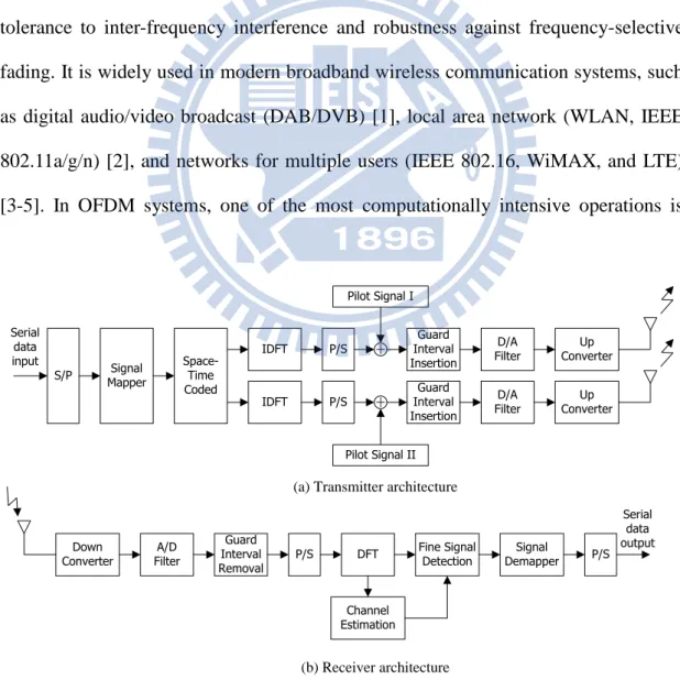
Digital signal processing (DSP) algorithms have become the foundation of today’s audio/video and communication systems. The well-known DSP algorithms, including finite-impulse-response (FIR) filters and fast Fourier transform (FFT), have attracted the attentions of a number of researchers over several decades. For example, orthogonal frequency-division multiplexing (OFDM) is known for the advantages of tolerance to inter-frequency interference and robustness against frequency-selective fading. It is widely used in modern broadband wireless communication systems, such as digital audio/video broadcast (DAB/DVB) [1], local area network (WLAN, IEEE 802.11a/g/n) [2], and networks for multiple users (IEEE 802.16, WiMAX, and LTE) [3-5]. In OFDM systems, one of the most computationally intensive operations is
S/P MapperSignal IDFT IDFT P/S P/S Guard Interval Insertion Guard Interval Insertion D/A Filter D/A Filter Up Converter Up Converter + + Pilot Signal II Pilot Signal I Serial data input Down
Converter FilterA/D
Guard Interval
Removal DFT P/S
Fine Signal
Detection DemapperSignal P/S Serial data output Channel Estimation
(a) Transmitter architecture
(b) Receiver architecture
Space-Time Coded
modulation/demodulation, which requires the filters to maximize the signal-to-noise ratio (SNR) and a dedicated FFT processor for discrete Fourier transform (DFT) computation [5-7]. Figure 1 illustrates an example of a pilot-based STBC/OFDM transmitter and receiver communication architecture [8]. Since the filter and FFT are required for processing each stream data, they are obviously the major computation blocks in a high-data-rate baseband system. Also note that, the area of the FFT core is reported about 25% of that of an IEEE 802.11a baseband processor [9, 10]. Thus, the DSP algorithms, such as the filter and FFT cores, must be carefully designed to minimize the hardware cost.
1.1 MCM-Based FIR Designs
For most of DSP algorithms, multiplication is one of the most frequently-used essential operations. For example, each input of an N-tap FIR filter should be multiplied by N constant coefficients. The multiplication between an input data value and a set of constants is also referred to as the multiple constant multiplication (MCM). Since the multiplier is not a small functional unit in hardware implementation, its usage should be reduced whenever possible. Meanwhile, a constant multiplication can actually be accomplished through a set of adders along with proper bit shifting rather than a real multiplier. For instance, a constant multiplication that always multiplies the input value x by 5 (i.e., y = 5 x) can be computed as y = (x << 2) + x. That is, a regular multiplier can be safely replaced with just an adder. Note that shifting a value by a fixed number of bits can be simply achieved via signal wiring in hardware implementation, which is virtually at no cost. As compared with the trivial implementation using a regular multiplier, it is obvious that the one with adders can usually reduce the hardware cost. Moreover, the area saving is likely to be more significant if the multiplication results with multiple
constants are required simultaneously. For example, two constant multiplications, y1 =
5 × x and y2 = 13 × x, can be accomplished by only two adders: y1 = (x << 2) + x and
y2 = (x << 3) + y1. Consequently, the notion of multiplier-less MCM has been widely
adopted for implementing area-efficient digital filters.
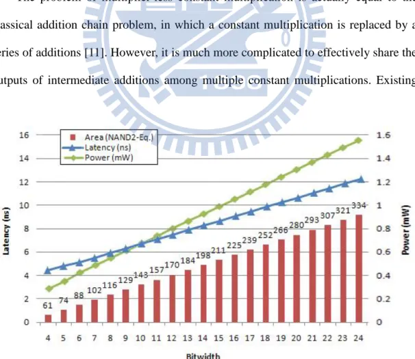
For an adder, the bitwidth is directly proportional to its area, delay, as well as power. For example, Figure 2 illustrates the area, latency, and power consumption of a ripple carry adder under the TSMC 0.18μm technology. The area, power consumption, and latency of an 8-bit adder are 116 gates, 0.55 mW, and 5.9 ns, respectively, which are approximately half of those of a 16-bit adder (225 gates, 1.05 mW, and 10.2 ns). Therefore, it is crucial to take the adder bitwidth into account very seriously while implementing a multiplier-less MCM block since it is solely made of adders.
The problem of multiplier-less constant multiplication is actually equal to the classical addition chain problem, in which a constant multiplication is replaced by a series of additions [11]. However, it is much more complicated to effectively share the outputs of intermediate additions among multiple constant multiplications. Existing
multiplier-less MCM algorithms for adder minimization can be divided into two major categories: 1) the graph-based algorithms [12-19], and 2) the digit-based algorithms [20-31]. Given a set of constants, a graph-based algorithm gradually builds the corresponding graph representation in a bottom-up fashion and uses some heuristic method to explore the chances for subexpression sharing among those constants. In general, they can provide a solution with fairly good quality in a short runtime; however, optimality is not guaranteed. In contrast, a digit-based algorithm generates a set of number decompositions for subexpression sharing based on a specific numeric representation. The ILP solver is sometimes utilized to produce an adder-minimal solution [23, 27-30] at the cost of longer runtime [32, 33].
Note that most of the previous studies regard the adder count minimization as the optimization goal and neglects the fact that every adder has its own area and delay cost due to different bitwidth. Hence, in this dissertation, we propose a new algorithm that minimizes the overall adder bitwidth instead of the total adder count. Meanwhile, the methods presented in the previous works [28, 29] use a pre-computed lookup table to store all feasible number decompositions of all constants within a fixed precision (e.g., 13 bits) no matter they are required or not. In contrast, our algorithm dynamically creates a subexpression graph that merely contains necessary information. The experimental results demonstrate that our algorithm can achieve a reduction on the total adder bit count by up to 10% for some test cases as compared with the existing state-of-the-art techniques. The details of the proposed ILP-based bitwidth-aware subexpression sharing algorithm are elaborated in Chapter 2.
1.2 FFT Architectures and Designs
An FFT core has several important design parameters, such as base
[34], various architectures have been developed and optimized for different goals. The architectures of FFT processors can be roughly divided into two major categories: memory-based and pipeline-based. Memory-based architectures usually consist of a butterfly unit and certain number of memory blocks for providing low-cost designs. However, it is very difficult for them to achieve real-time processing at low clock frequency. Alternatively, a pipelined architecture consists of multiple stages to provide higher throughput at the cost of more hardware. In general, memory-based architectures are suitable for FFT processors where the hardware cost is an issue and the FFT size is not smaller than 512 [3]. Pipeline-based architectures are typically feasible for applications with smaller FFT sizes. Meanwhile, the proper FFT size varies for different applications. For example, the size can be 128, 256, 512, 1024, or 2048 for WiMAX applications; and 256, 512, 1024, or 2048 for DAB systems. Hence, for a specific application, the requested FFT core should be well configured to meet its own unique requirements.
Many pipelined FFT architectures [35-44] have been proposed in past few decades. For a specific architecture, one way to accelerate its computation is to increase the clock rate. For example, the conventional Radix-2 Multi-path Delay Commutator (R2MDC) takes 1023 clock cycles for a 1024-point FFT computation. Assume that a butterfly operation takes 20 ns in a given technology; and as a result the execution time of a complete 1024-point FFT computation requires 20.5 us. If the system requires even faster response time (< 20.5 us), a higher operation frequency is demanded. The other way to provide higher throughput is to expand the datapath of the original architecture. However, expanding a pipelined FFT architecture is not always trivial because of internal dissimilar data permutation patterns and complicated controlling logic. The difficulty generally increases as the
degree of parallelism rises. Thus, a generator that can automatically provide those expanded architecture variants is demanded for saving design costs drastically. To deal with this issue, in this dissertation we propose an Expandable Multi-path Delay Commutator (EMDC) based FFT architecture and the corresponding generator targeting high-performance applications. Due to the page limitation, we only demonstrate the details of the proposed Radix-22EMDC architecture in Chapter 3. However, the proposed approach can be easily applied to other MDC-based architectures, such as Radix-23MDC and Radix-24MDC.
Furthermore, the scaling optimization on FFT designs with a fixed wordlength at each stage needs to be considered; that is, the output wordlength of every stage is the same as its input wordlength. Memory-based designs naturally fulfill this requirement, while a considerable part of pipeline-based designs also choose to meet the same requirement since the fixed wordlength is still preferred due to hardware cost and critical-path delay considerations.
While crafting a practical FFT hardware design, the output precision in terms of signal-to-quantization-noise (SQNR) ratio is regarded as a key design requirement. In practice, FFT algorithms are commonly implemented using fixed-point arithmetic instead of floating-point arithmetic for hardware cost reduction. That is, only a limited number of bits are available to represent a signal or coefficient value. As a result, rounding and truncation operations inevitably introduce noises, which are referred to as quantization noises. Besides, addition and subtraction operations may also cause overflow errors (noises) during computations. Although extending the wordlength can relieve the accuracy loss, the hardware cost and the critical-path delay are increased accordingly.
Therefore, several number scaling methods, either static or dynamic, have been proposed to improve the output SQNR [1, 45-64]. Oppenheim et al. [49]
proposed a simple static scaling method that always increases the integer part by one bit for each radix-2 stage to prevent overflows. However, this method suffers significant quantization errors if the wordlength is fixed. In addition, methods based on dynamic scaling have also been proposed for the SQNR improvement. Block Floating Point (BFP)-based methods employ intermediate buffers to store and analyze a block of output values, and then dynamically determine an appropriate number format for that block to achieve a better SQNR [1, 45, 46, 51, 52]. However, all of these dynamic methods suffer a notable increase in area, power, and latency as well as need a more complicated control unit to achieve a similar quality of result (QoR). Consequently, most FFT designers rely on static instead of dynamic scaling optimization techniques to determine a proper number format for each stage [50].
Previous static scaling techniques can be roughly classified into three major categories: simulation-based approaches [58, 59], analytical approaches [47, 49, 50, 60-68], and a hybrid of previous two [48, 69, 70]. The simulation-based approaches try to find a good number format through lengthy iterations. In contrast, the analytical methods can determine a good number format very efficiently through a static numeric analysis without invoking time-consuming simulation. However, the analysis results are generally too pessimistic and lead to a larger wordlength than required. Therefore, the hybrid approaches are proposed to determine the number format and shorten the simulation time simultaneously. Meanwhile, the works mentioned above [47-50, 58-70] all assume they can arbitrarily determine the wordlength at each stage. However, in memory-based FFT designs, the wordlength (the width of the memory block) is always fixed. To the best of our knowledge, the problem of static scaling under a fixed wordlength constraint has not been well addressed yet.
In this dissertation, we propose a scaling optimization technique based on the static probability analysis that can rapidly determine the best number format at each butterfly stage under a fixed wordlength constraint. Given a probability distribution of input signals, a selected FFT algorithm, and a wordlength constraint, the proposed technique can maximize the overall output SQNR through the static number format analysis and optimization stage by stage. Compared to previous works, our method offers the following three contributions: 1) providing a probability model that can abstract the behavior of fixed-point arithmetic logic; 2) preventing the use of time-consuming and pattern-dependent simulation throughout the entire optimization process; 3) minimizing the required wordlength in a hardware implementation under a given SQNR target without demanding extra hardware components and complicating control logic compared to other existing static approaches [49, 50].
1.3 Dissertation Organization
The rest of this dissertation is organized as follows. In Chapter 2, an ILP-based bitwidth-aware subexpression sharing for area minimization in filter design is presented. In Chapter 3, we demonstrate an expandable MDC-based FFT architecture and its generator targeting for the high-performance applications. Then, a probability-based static scaling optimization flow for fixed wordlength FFT processors is developed in Chapter 4. Finally, the concluding remarks and the future works are given in Chapter 5.
Chapter 2
Bitwidth-Aware Subexpression
Sharing in FIR Filter
2.1 FIR Filter Implementation
In this section, we first introduce the fundamentals of an FIR filter design. Then, three different number representations as well as the related algorithms are briefly reviewed here.
2.1.1 Fundamentals of FIR filter design
A general form of a linear time-invariant N-tap FIR filter can be expressed as a convolution involving the last N input data and N constant filter coefficients. The output y(n) can be calculated as:
1 0 ( ) ) ( N k ck x n k n y (1) where1. x(n) is the input sequence,
2. y(n) is the corresponding output sequence,
3. ck are constant filter coefficients, and 4. N is the filter length.
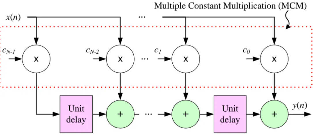
Figure 3 illustrates a general fully-parallel transposed architecture of FIR filter, which requires N–1 additions and N multiplications to produce a single output value. It is also observed that one of the two inputs of every multiplication is always from the
present input sample. Therefore, an MCM block can be used to produce a set of products between an input value and a given set of constant coefficients. Since all coefficients are fixed-point constants, those constant multiplications can be solely achieved through a series of additions, and thus the use of costly regular multipliers can be completely eliminated as previously mentioned
2.1.2 Number representations
Three different number formats can be used to represent fixed-point constants: pure binary form, the canonical signed digit (CSD) form, and the minimal signed digit (MSD) form. The pure binary form is the trivial unsigned binary representation, where every digit is either 0 or 1. In the CSD representation, three symbols, 0, 1, and 1, are used, where 1 denotes –1. The CSD representation has the following two properties: 1) the count of nonzero digits (i.e., 1 and 1) is minimal; and 2) any two adjacent digits cannot both be nonzero. In addition, the CSD representation for a
Table 1 Three different representations for the number 23 Representation
pure binary 010111
CSD 101001
MSD 011001 or 101001
Figure 3 A general architecture of FIR filter.
x + x + x + x x(n) cN-1 cN-2 … c1 c0 y(n) Unit delay Unit delay … …
number is unique, and this is how “canonical” comes from. Similar to the CSD form, the MSD form also adopts the same three symbols and requires that the count of nonzero digits is minimal. Unlike the CSD from, the MSD form allows adjacent nonzero digits, which makes itself no longer a canonical representation. In other words, a number may have multiple valid MSD representations. Note that the CSD representation is also a valid MSD representation. Table 1 gives an example where the number 23 is presented in those three representations with the length of six digits. The number 23 has a unique representation in pure binary form and CSD form, but has two feasible representations in MSD form. Besides, it is a guarantee that for any number the count of nonzero digits in pure binary representation is no less than that in CSD and MSD representations.
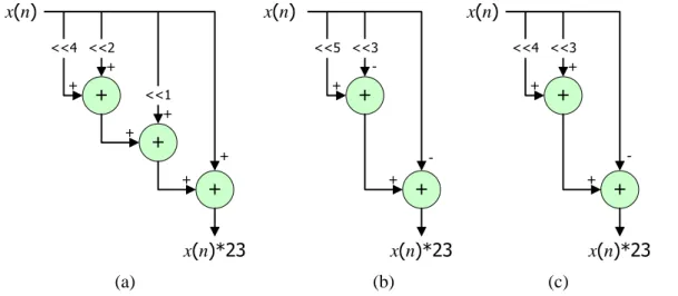
In hardware implementation, the count of nonzero digits of a value c basically determines the number of required additions to realize the multiplication by c. Figure 4 demonstrates three different ways for implementing a constant multiplication by 23. Figure 4(a) shows a direct implementation based on the pure binary representation (i.e., 10111). Since there are four nonzero digits, three adders are required to complete the multiplication (i.e., 23x=16x+4x+2x+x). However, there are only three nonzero
(a) (b) (c) + + + x(n)*23 <<1 <<2 <<4 + + + + + + x(n) x(n) + + x(n)*23 <<5 <<3 -+ -+ + + x(n)*23 x(n) <<4 <<3 + + -+
digits if the CSD format is considered (i.e., 101001). As shown in Figure 4(b), merely two adders are enough to accomplish the same multiplication (i.e., 23x=32x–8x–x, a subtraction a – b is regarded as an addition a + (–b) in this dissertation). Since the number 23 has two valid MSD representations, Figure 4(c) illustrates the other one (i.e., 011001), which also needs two adders only (i.e., 23x=16x+8x–x). Consequently, CSD and MSD representations are usually adopted in constant multiplications because both of them guarantee the count of nonzero digits for any given constant is always minimal.
2.1.3 Digit-based algorithms
A number of algorithms have been proposed to decompose a set of constants based on a specified number representation [20-33]. However, most of these previous methods only focus on the minimization of the total adder count. Since the area and delay of an adder is highly dependent on the bitwidth as mentioned, it is unwise to neglect its impact during optimization. For example, two different ways can be used to implement the constant multiplication of 11x: (1x+2x)+8x or (1x+8x)+2x. They both require two adders to complete the multiplication. However, the bitwidth of the result of (1x+8x), is apparently longer than that of (1x+2x). Since a wider result potentially requires wider adders for succeeding additions, it is actually a good idea to take the resultant bitwidth of addition outcome into account for better optimization outcomes.
2.1.4 Motivation of our work
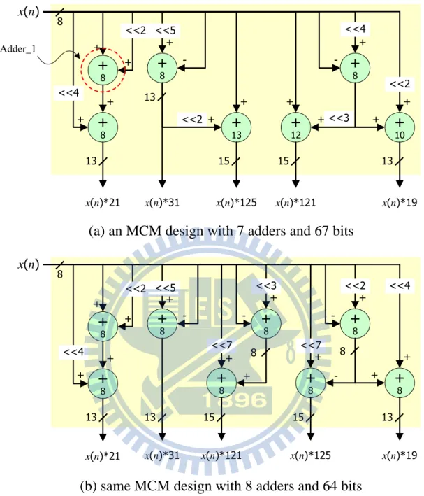
Figure 5 (a) illustrates a sample multiplier-less MCM design, where the input x is 8-bit wide. Instead of using five costly multipliers, the five output values (the input x times 19, 21, 31, 121, and 125) can be produced by only seven adders.Note that every
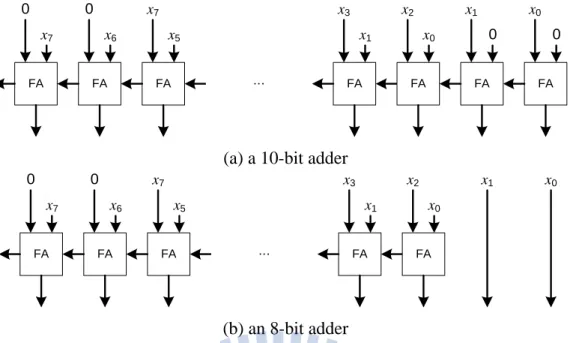
adder must be wide enough to ensure the absence of overflow. Typically, an adder with n–1 bits is used to generate an n-bit sum. For example, Adder_1 shown in Figure 5(a) is used to produce an output of 5x = x + (x << 2), where the output is 11-bit wide and the trivial implementation of Adder_1 should be 10-bit wide, as depicted in Figure 6 (a). However, it is observed that the rightmost two adder bits in Figure 6(a) are actually redundant due to the 2-bit right shifting (i.e., x << 2). As a consequence, Adder_1 can be safely downsized to an 8-bit adder, as shown in Figure 6(b). This example clearly indicates that a more compact adder implementation can possibly be achieved if the relation between two input operands is carefully investigated.
Let us reexamine the implementation shown in Figure 5(a). The number labeled within a circle specifies the minimal bitwidth of the corresponding adder. Hence, a total of 67 bits is required for those 7 adders. Meanwhile, Figure 5(b) illustrates another implementation for the same MCM, which requires 8 adders but only 64 adder bits. That is, the implementation depicted in Figure 5(b) consumes more adders but less adder bits than that shown in Figure 5(a). As previously explained, we consider the solution given in Figure 5(b) is better. However, those previous approaches trying to minimize the adder count would prefer the solution shown in Figure 5(a). Consequently, it motivates us to develop a new area minimization algorithm for MCM designs that concentrates on total adder bitwidth minimization. The details are elaborated in the following two sections.
(a) an MCM design with 7 adders and 67 bits
(b) same MCM design with 8 adders and 64 bits
+
8+
13+
8+
10+
12 x(n) x(n)*125 x(n)*31 x(n)*121 x(n)*19 8 15 13 15 13 <<5 + <<2 + + <<4 + -<<2 <<3+
8+
8+
8+
8+
8 x(n) x(n)*31 x(n)*121 x(n)*125 x(n)*19 8 13 8 15 13 8+
8 <<5 + -<<3 <<2 + -+ -<<7 + + <<4 + + + -<<7+
8 + -<<2 ++
8 x(n)*21 13+
8 + <<2 ++
8 x(n)*21 13 + + + + <<4 15 <<4 Adder_1 + + + +(a) a 10-bit adder (b) an 8-bit adder FA FA FA FA FA FA x0 x1 x3 x7 0 0 x5 x6 x7 x1 0 0 FA x2 x0 … FA FA FA FA x0 x1 x3 x7 0 0 x5 x6 x7 x1 FA x2 x0 …
2.2 Proposed Algorithm
In this section, we present a bitwidth-aware ILP-based area minimization algorithm for MCM designs. It uses a graph-based approach that keeps track of common subexpressions among constants as well as calculates the exact required bitwidth of each adder simultaneously. The details are described in the following sections.
2.2.1 Number decomposition and bitwidth calculation
The fundamental of the MCM optimization problem is to maximize the common subexpression sharing among given constants. Hence, it is generally true that the optimization outcome could be better if more ways are considered for decomposing a constant, i.e., a larger solution space. However, the number of possible ways for decomposing a number is actually infinite. For example, the number 3 can be achieved as 1+2, 4–1, 5–2, 6–3, 7–4, and so on. Fortunately, not all of them are appropriate while constructing an area-efficient solution. As explained in Section 2.2, the number of adders (Az) needed to accomplish a constant multiplication by z is equal to the number of nonzero bits of z (Bz) minus one, i.e., Az = Bz – 1. Hence, there is no reason to decompose z as x + y if Bz < Bx + By during optimization. For instance, it is not wise to decompose the number 3 as 5–2. In our method, a set of target constants D = {di} is first converted into C = { ci | di = ci 2l, ci is an odd number}. That is, all constants ci are assumed odd numbers initially. Next, for every constant c with k (where k > 1) nonzero digits in its MSD representation, the proposed algorithm merely considers a finite set of number decompositions complying with the following format:
0 , 2 d e d f l c l (2)
where d and f must be odd, as well as e must be even.
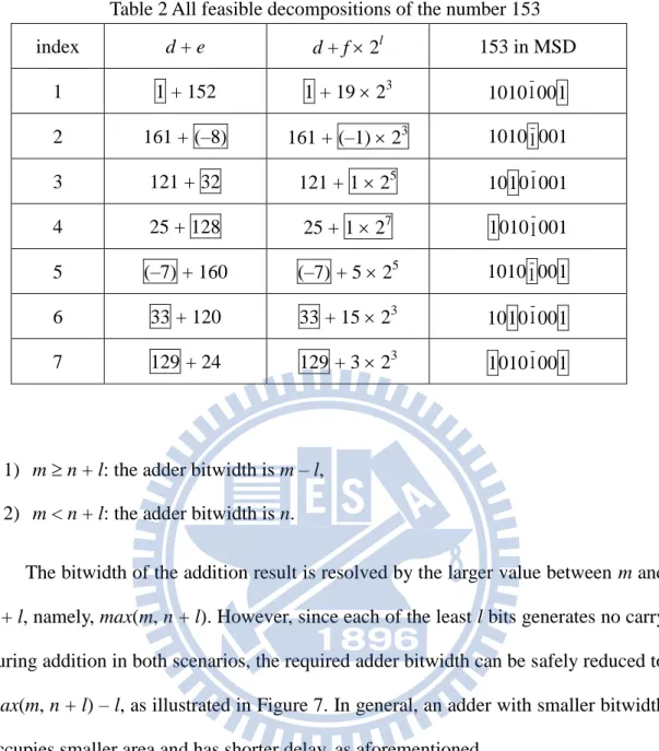
For example, the set of decompositions for the number 153 (10101001 in MSD) is enumerated in Table 2. Actually, a number decomposition c = d + e is created by partitioning the nonzero digits in c’s MSD form into two nonempty disjoint groups. The group contains the least significant digit (LSD) actually defines the value of d (odd), while the other group specifies the value of f (even). As shown in the last column of Table 2, the nonzero digits are partitioned into gray and non-gray groups. Therefore, for a number c that has m valid MSD representations and every one includes k nonzero digits, the total number of possible decompositions of c can be formulated as:
2 1
2 2 1 1 2 1 2 1 1 0
k k i m i k m k k k k m (3)For instance, the total number of decompositions for 153 is 1(24–1–1) = 7 according to (3).
For a decomposition c = d + f 2l, both |d| and |f| are called the subexpressions of
c. For example, the number 153 has eleven different subexpressions – {1, 3, 5, 7, 15,
19, 25, 33, 121, 129, 161}. Hence, according to (2), the decompositions and the subexpressions of any odd number larger than 1 can be identified using the approach described above.
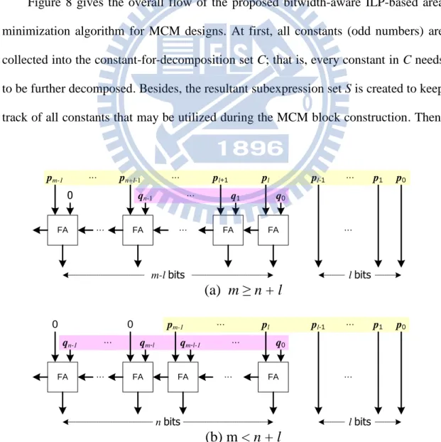
An adder is required to carry out a decomposition of a constant multiplication cx = dx + fx 2l = p + (q << l). Assume p is m-bit long and q is n-bit long, the adder bitwidth can thus be determined based on the following two scenarios:
1) m n + l: the adder bitwidth is m – l, 2) m < n + l: the adder bitwidth is n.
The bitwidth of the addition result is resolved by the larger value between m and
n + l, namely, max(m, n + l). However, since each of the least l bits generates no carry
during addition in both scenarios, the required adder bitwidth can be safely reduced to
max(m, n + l) – l, as illustrated in Figure 7. In general, an adder with smaller bitwidth
occupies smaller area and has shorter delay, as aforementioned.
While revisiting the previous decomposition example of 153, we further assume the input x is 8-bit wide, which is used to produce the output 153x. By Table 2, a possible decomposition is 153 = 121 + 32 = 121 + 1 25, which indicates that the output 153x can be obtained from the summation of 121x and 32x. Obviously, 32x is only 5-bit left shift of x. Also note that the left shift requires no additional hardware in the real implementation. Meanwhile, 121x needs to be further decomposed based on (2) in the same manner and its bitwidth is 15 bits (i.e., 8 + log2121). The adder type
required to sum up 121x and 32x is the one illustrated in Table 7(a), where m = 15, n = Table 2 All feasible decompositions of the number 153
index d + e d + f 2l 153 in MSD 1 1 + 152 1 + 19 23 10101001 2 161 + (–8) 161 + (–1) 23 10101001 3 121 + 32 121 + 1 25 10101001 4 25 + 128 25 + 1 27 10101001 5 (–7) + 160 (–7) + 5 25 10101001 6 33 + 120 33 + 15 23 10101001 7 129 + 24 129 + 3 23 10101001
8, and l = 5. Therefore, the required bitwidth of the adder is 15 – 5 = 10 bits.
On the other hand, 153 can also be decomposed in the form of 153 = 25 + 128 = 25 + 1 27, which implies 153x comes from adding 25x from 128x. Similarly, 128x is merely 7-bit left shift of x and 25x is 13-bit wide (i.e., 8 + log225). Alternatively,
the adder type required to sum up 25x and 128x is the one shown in Figure 7(b), where m = 13, n = 8, and l = 7. Consequently, the required bitwidth of the adder is 8 bits.
2.2.2 Bitwidth-aware multiplier-less MCM design flow
Figure 8 gives the overall flow of the proposed bitwidth-aware ILP-based area minimization algorithm for MCM designs. At first, all constants (odd numbers) are collected into the constant-for-decomposition set C; that is, every constant in C needs to be further decomposed. Besides, the resultant subexpression set S is created to keep track of all constants that may be utilized during the MCM block construction. Then,
(a) m ≥ n + l
(b) m < n + l
FA FA FA … FA pl pm-1 0 0 qm-l-1 qm-l qn-1 q0 pl-1 p1 p0 … … l bits n bits … … … … FA FA FA … FA pl pm-1 q1 0 q0 pl-1 p1 p0 … l bits m-l bits … pl+1 … qn-1 … pn+l-1 … …an arbitrary constant c is removed from C for decomposition. Based on the specified number representations, i.e., pure binary, CSD, or MSD, all decompositions of c are enumerated and the associated hardware cost in terms of total adder bit count is calculated using the method presented in Section 3.1.
Next, c is added into S after all decompositions of c are identified. For every subexpression of c that has not been present in S yet, it is added into D for further decomposition. This process is not terminated until D is empty. As a result, the set S contains all possible constant numbers that may appear in the final MCM block.
While performing constant number decomposition, the proposed approach concurrently builds a subexpression graph to keep track of all feasible decompositions for a given constant c. The graph also records the cost of every decomposition (i.e., adder bit count). Finally, based on this subexpression graph, a set of corresponding ILP constraints can be derived and then an ILP solver is utilized to produce an MCM design solution with the minimal total adder bits. The details of the ILP formulations are given in Section 4 later. Conventional look-up table based approaches require a
1. C { all constant numbers } 2. S { 1 }
3. while ( C is not empty )
4. Remove an arbitrary constant c from C 5. Add c into S
6. foreach ( decomposition d of c )
7. Identify two subexpressions s & t of d 8. Calculate the required adder bit count 9. Record d in the subexpression graph G 10. Add s & t into C if they are not in S yet 11. Derive ILP constraints from G
12. Find a solution with minimal adder bit count by ILP Figure 8 The proposed algorithm flow.
pre-computed table to store all decompositions of every odd number within a fixed bitwidth (e.g., 13-bit). Therefore, the table can become very huge as the bitwidth increases. In contrast, the proposed algorithm merely enumerates decompositions for a limited number of subexpressions.
2.3 Example of Subexpression
Graph Construction
In this subsection, the CSD representation is in use for simplicity. Note that the proposed algorithm is applicable to the MSD one. We also use an example to demonstrate how a subexpression graph is dynamically constructed. In the following example, the 8-bit input is multiplied by two constant numbers, 21 and 153. First, these two constants are transformed in CSD form.
CSD 2 10 CSD 2 10 001 1 1010 10011001 153 and 10101 10101 21
According to its CSD form, each constant can be further decomposed as a set of subexpressions based on the method described in Section 3.1
3 3 5 7 5 3 3 4 2 2 2 3 129 2 15 33 2 5 7 2 1 25 2 1 121 2 1 161 2 19 1 153 and 2 1 5 2 1 17 2 5 1 21
There are three and seven decompositions for 21 and 153, respectively, which is the same as (3) specifies. After decomposition, we also find that the number 21 has three subexpressions of {1, 5, 17} and the number 153 has eleven subexpressions of {1, 3, 5, 7, 15, 19, 25, 33, 121, 129, 161}. Every subexpression (except 1) needs to be further decomposed for finding out all its feasible decompositions and the associated
adder bit count, as the algorithm flow presented in Figure 8.
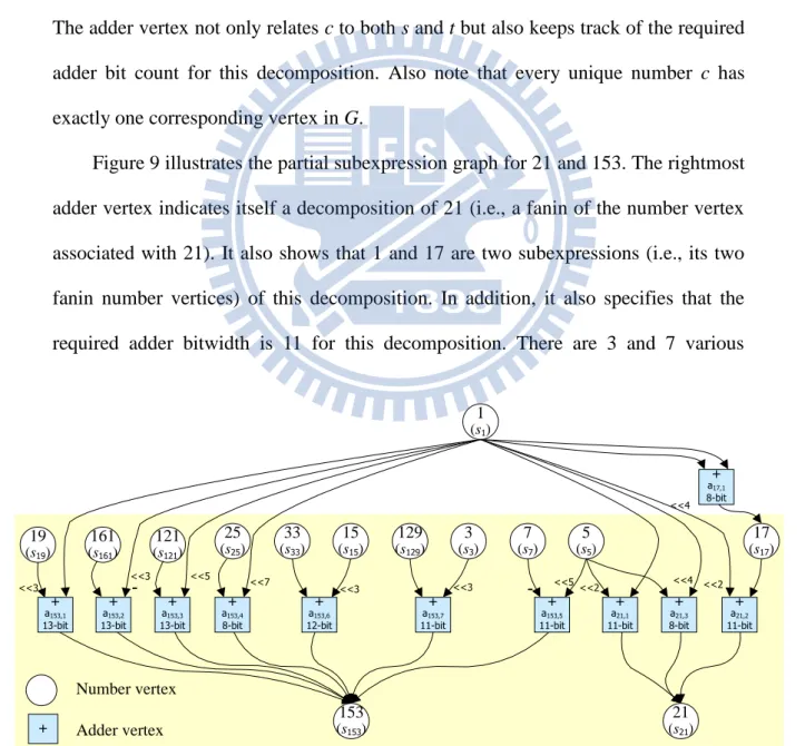
There are two types of vertices within a subexpression graph G: 1) a number vertex is associated with a constant value, and 2) an adder vertex specifies a decomposition and associates the decomposed number with its two subexpressions. When a constant number c is removed from C, a corresponding number vertex is added into G if it is not present in G. For every feasible decomposition of c, a corresponding adder vertex is added into G. Similarly, a number vertex associated with each of two subexpressions, s and t, is also inserted into G if it is not present in G. The adder vertex not only relates c to both s and t but also keeps track of the required adder bit count for this decomposition. Also note that every unique number c has exactly one corresponding vertex in G.
Figure 9 illustrates the partial subexpression graph for 21 and 153. The rightmost adder vertex indicates itself a decomposition of 21 (i.e., a fanin of the number vertex associated with 21). It also shows that 1 and 17 are two subexpressions (i.e., its two fanin number vertices) of this decomposition. In addition, it also specifies that the required adder bitwidth is 11 for this decomposition. There are 3 and 7 various
1 (s1) 19 (s19) 161 (s161) 121 (s121) 25 (s25) 7 (s7) 5 (s5) 33 (s33) 15 (s15) 129 (s129) 3 (s3) 153 (s153) 21 (s21) <<3 <<3- <<7 <<3 <<3 - <<5<<2 <<4 <<2 17 (s17) <<4 Number vertex Adder vertex + a153,1 13-bit <<5 + + a153,2 13-bit + a153,3 13-bit + a153,4 8-bit + a153,6 12-bit + a153,7 11-bit + a153,5 11-bit + a21,1 11-bit + a21,3 8-bit + a21,2 11-bit + a17,1 8-bit
decompositions for 21 and 153 respectively as shown in Figure 9. A subexpression larger than one should be further decomposed. Except for 17, Figure 9 does not show the succeeding decompositions due to page limitation. Note that Figure 9 also shows that 5 is a common subexpression of both 21 and 153, which implies the hardware cost may be reduced if 5 is shared by both of them in the final implementation. All chances of common subexpression sharing can be exhaustively identified in the proposed subexpression graph.
2.4 ILP Formulation
The problem of bitwidth-aware area minimization for MCM design is thus solved through integer linear programming (ILP). Three types of constraints are derived: 1) an existence constraint guarantees at least one of decompositions is selected for a specified number, 2) a dependency constraint ensures the two corresponding subexpressions would also be implemented if a specified decomposition is selected, and 3) an output constraint guarantees all the output constants of the given MCM are implemented. The ILP-related notations used in this section are given below.
sn: a 0-1 variable indicating if the subexpression of the value n is implemented. dn: the count of feasible decompositions of the number n.
an,i: a 0-1 variable indicating whether the i-th decomposition of the number n is selected for implementation.
bn,i: the required adder bit count for implementing the i-th decomposition of the number n.
2.4.1 Existence constraints
must be selected for implementation, which can be formulated as the following constraint:
}
{
, 1 i d ni nmax
a
s
n
(4)For example, there are three different decompositions for the number 21, as shown in Figure 9. According to (4), at least one of those three decompositions must be selected. That is,
}
,
,
{
}
{
21, 21,1 21,2 21,3 3 1 21max
a
max
a
a
a
s
i i
2.4.2 Dependency constraints
As explained in Section 2.3, a decomposition actually implies an adder and its two subexpressions serve as the inputs to the adder. Hence, there is no way to get the addition outcome if those two inputs are not available. That is, if the i-th decomposition of the number n is selected for realization, both of its two corresponding subexpressions, x and y, must also be carried out. The constraint can then be formulated as:
}
,
{
,i x y nmin
s
s
a
(5)For instance, the number 153 can be regarded as 3
2 15
33 by the sixth decomposition of 153 shown in Figure 9. Hence, the corresponding dependency constraint can be given as:
}
,
{
33 15 6 , 153min
s
s
a
2.4.3 Output constraint
Assume that the set C includes all constant numbers of the target MCM block; the following output constraint is applied to ensure that every element n C is properly implemented:
C
n
s
n
1
,
(6)2.4.4 Optimization goal
As aforementioned, the hardware cost of the target MCM block can be lowered if the total adder bit count in use can be minimized. Since every implemented adder must be associated with a variable an,i set to 1 and the bitwidth of that adder is bn,i, the goal of total adder bitwidth minimization can thus be accomplished through setting the objective of the ILP formulation as:
minimize
C n i d i n i n nb
a
1 , , (7) subject to (4), (5), and (6).2.5 Experimental Results
To evaluate the proposed algorithm, we compare it against a widely used graph-based technique revealed in [14] as well as a state-of-the-art digit-based technique presented in [29]. All experiments have been conducted on a Linux platform with two Intel Xeon 2.4 GHz processors and 12 GB main memory. For the preparation of test cases, the Remez algorithm [51, 52] is utilized to randomly generate FIR filters of various types, including low-pass, high-pass, band-pass, and band-stop. Besides, the MSD representation is adopted for the number decomposition,
and the Gurobi Optimizer [53] is used as ILP solver.
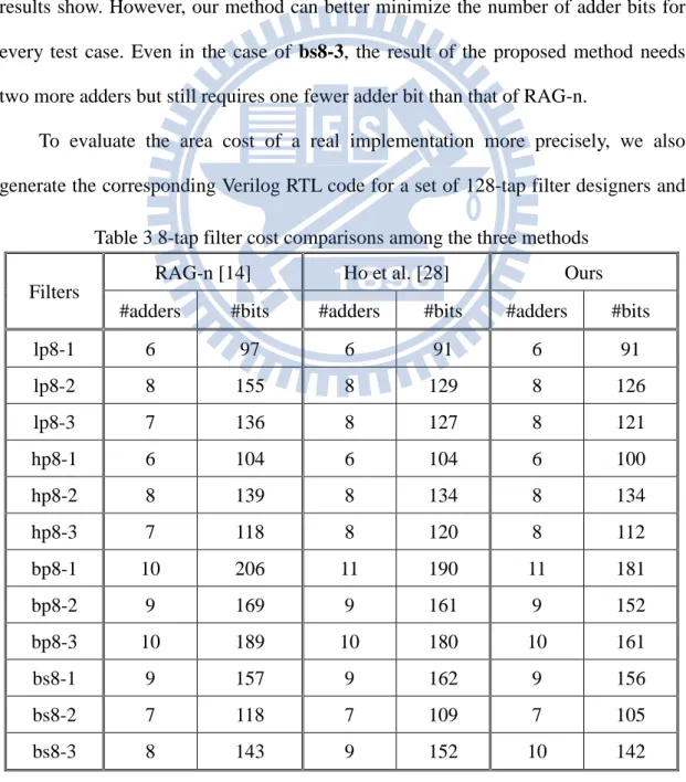
In Table 3, 12 8-tap filters are evaluated with 12-bit coefficients and input data. For each method, #adders reports the total number of adders required in the MCM block, while #bits gives the total number of adder bits. Since RAG-n [14] allows the use of right shifters and accepts a mapping result that induces extra adders for a coefficient to maximize global subexpression sharing, it is capable of finding a design solution that is not presented in the solution space for digit-based algorithms. Hence, RAG-n is likely to better minimize the number of adders for an MCM design, as the results show. However, our method can better minimize the number of adder bits for every test case. Even in the case of bs8-3, the result of the proposed method needs two more adders but still requires one fewer adder bit than that of RAG-n.
To evaluate the area cost of a real implementation more precisely, we also generate the corresponding Verilog RTL code for a set of 128-tap filter designers and
Table 3 8-tap filter cost comparisons among the three methods Filters
RAG-n [14] Ho et al. [28] Ours #adders #bits #adders #bits #adders #bits
lp8-1 6 97 6 91 6 91 lp8-2 8 155 8 129 8 126 lp8-3 7 136 8 127 8 121 hp8-1 6 104 6 104 6 100 hp8-2 8 139 8 134 8 134 hp8-3 7 118 8 120 8 112 bp8-1 10 206 11 190 11 181 bp8-2 9 169 9 161 9 152 bp8-3 10 189 10 180 10 161 bs8-1 9 157 9 162 9 156 bs8-2 7 118 7 109 7 105 bs8-3 8 143 9 152 10 142
then synthesize the RTL code into the gate-level design based on TSMC 0.18m technology. In Table 4 and Table 5, two configurations with different coefficient widths, 12-bit and 16-bit, are examined for each filter. In addition, the input is also assumed as wide as the coefficient. Similarly, #adders reports the total number of adders in the MCM block, #bits gives the total number of adder bits, and #gates reveals NAND2-equavilent gate count in the synthesized circuit. Table 4 clearly shows that for every test case the proposed algorithm needs more or same number of adders than the method in [28].
However, our method requires fewer adder bit count in every test case. For 12 12-bit test cases in Table 4, the average reductions on the adder bit count and the gate count are 7.38% and 7.91%, respectively; for 12 16-bit test cases in Table 5, the corresponding reductions are 7.65% and 7.27%, respectively. Note that the
Table 4 Synthesis results and comparisons for 12-bit 128-tap FIR filters
Ho et al. [28] Ours Comparisons
#adders #bits #gates #adders #bits #gates #adders increased bit saving (%) gate saving (%) lp128-1 68 1,245 23,254 69 1,122 21,487 1 9.9 7.6 lp128-2 57 1,063 20,006 58 987 18,869 1 7.1 5.7 lp128-3 68 1,286 24,443 70 1,175 21,597 2 8.6 11.6 hp128-1 60 1,103 21,305 60 1,025 19,290 0 7.1 9.5 hp128-2 67 1,243 22,004 67 1,165 20,792 0 6.3 5.5 hp128-3 68 1,225 22,264 69 1,122 20,762 1 8.4 6.7 bp128-1 61 1,109 19,952 62 1,004 18,373 1 9.5 7.9 bp128-2 63 1,122 21,469 65 1,048 19,259 2 6.6 10.3 bp128-3 58 1,073 20,090 58 986 18,345 0 8.1 8.7 bs128-1 56 1,026 18,639 57 959 17,856 1 6.5 4.2 bs128-2 61 1,102 20,527 62 1,056 19,215 1 4.2 6.4 bs128-3 56 1,035 19,701 57 977 17,741 1 5.6 9.9
improvements basically remain unchanged as the width of constant number increases from 12-bit to 16-bit, which is a good trend for the future applications. The experimental results also verify that the total adder bit count can better estimate the area cost in a real hardware implementation than the total adder count only, as we claimed previously.
Besides, the proposed method can also adopt the maximum logic depth constraint described in [28] to guarantee the worst-case delay through adding extra depth-related constraints into the ILP formulations. Two different logic depth constraints are examined for comparisons using a set of 12-bit 32-tap FIR filters and the results are shown in Table 5. The average bit count reduction is similar to the previous experiment, which is 5.77% and 7.18% as the maximum logic depth is set to 4 and 5, respectively.
Table 5 Synthesis results and comparisons for 16-bit 128-tap FIR filters
Ho et al. [28] Ours Comparisons
#adders #bits #gates #adders #bits #gates #adders increased bit saving (%) gate saving (%) lp128-1 99 2,401 46,789 103 2,195 43,858 4 8.6 6.3 lp128-2 96 2,267 45,783 97 2,129 45,404 1 6.1 0.8 lp128-3 96 2,303 44,290 98 2,205 44,154 2 4.3 0.3 hp128-1 95 2,331 49,248 100 2,133 43,400 5 8.5 11.9 hp128-2 96 2,350 50,826 97 2,151 45,139 1 8.5 11.2 hp128-3 98 2,361 49,281 101 2,170 44,662 3 8.1 9.4 bp128-1 91 2,157 40,536 92 1,996 38,147 1 7.5 5.9 bp128-2 95 2,324 48,145 99 2,094 42,598 4 9.9 11.5 bp128-3 92 2,235 46,108 96 2,067 42,869 4 7.5 7.0 bs128-1 87 2,157 45,151 88 1,975 42,579 1 8.4 5.7 bs128-2 93 2,274 46,591 98 2,104 43,656 5 7.5 6.3 bs128-3 93 2,215 46,102 94 2,061 41,755 1 7.0 9.4
In addition, all the ILP problems (including 12-bit and 16-bit 128-tap filters) presented in the experiments can be successfully resolved in less than an hour, which should be considered acceptable. As a consequence, it is conclusive that our proposed algorithm can produce better area-minimized MCM design solutions than the best prior art [29] within an acceptable runtime.
2.5 Summary
In this dissertation, we present an ILP-based bitwidth-aware area minimization algorithm for MCM designs. We first point out that the total adder bit count rather than the total adder count can better estimate the hardware cost in a real implementation. Then, for a given MCM design, those target constants are first represented in a specified number format (MSD in use in this dissertation). Next, a
Table 6 Logic depth comparisons for 12-bit 32-tap FIR filters
Filters
Depth = 3 Depth = 4
Ho et al. [28] Ours Ho et al. [28] Ours #adders #bits #adders #bits #adders #bits #adders #bits
lp32-1 16 282 16 271 16 296 16 271 lp32-2 21 363 21 323 21 354 21 323 lp32-3 15 259 15 241 15 250 15 241 hp32-1 22 405 22 373 22 400 22 373 hp32-2 17 294 17 284 17 300 17 284 hp32-3 19 339 19 318 19 334 19 318 bp32-1 25 421 26 382 24 388 24 378 bp32-2 22 399 23 393 21 384 22 373 bp32-3 23 395 23 366 23 417 23 366 bs32-1 23 405 23 346 23 393 23 346 bs32-2 24 419 24 368 23 381 24 368 bs32-3 21 360 21 328 21 356 21 328
subexpression graph is created to record all feasible decompositions for every target constant. The graph also keeps track of the required adder bitwidth as well as two subexpressions for every decomposition. At last, the area minimization problem is formulated as a set of ILP constraints derived from the subexpression graph and optimally resolved within an acceptable runtime. The experimental results demonstrate that our proposed algorithm can achieve an average reduction of more than 7% on both of the adder bit count and the real gate count. Therefore, we are confident that the proposed approach can outperform the existing state-of-the-art techniques and should be regarded as a better alternative for area minimization in MCM designs
Chapter 3
Expandable MDC-Based FFT
3.1 Overview of the Pipelined FFT Architecture
Pipelined architectures can be divided into two major categories according to the datapath structure. One is Single-path Delay Feedback (SDF) based architecture and the other is Multi-path Delay Commutator (MDC) based architecture. SDF-based architectures use properly-sized local delay feedback loops to correctly schedule the input data for butterfly units. It typically has the advantages of higher hardware utilization rate and less hardware cost. On the contrary, MDC-based architectures first separate the input sequence into two parallel data streams by properly-controlled switches/FIFOs and then direct them into the correct butterfly units. As a result, MDC-based architectures generally demand a bit more hardware resources and larger memory bandwidth but provide higher throughput in return. Nevertheless, though a fixed MDC-based architecture can generally provide good throughput at reasonable hardware cost, it may still fail to meet the target performance requirement for some throughput-hungry design cases.
In [54] and [55], a foldable structure is proposed to provide various design tradeoffs between area and throughput based on the base (Pease) architecture. Since the Pease architecture possesses high regularity, it is extremely easy to fold butterfly units in its implementation either horizontally or vertically. Figure 10 illustrates the fully-expanded 16-point foldable Pease FFT implementation. It is apparent that 4 butterfly columns are identical and thus can be easily 2- or 4-folded horizontally.
Similarly, identical 8 butterfly rows can be 2/4/8-folded vertically as well. With this folding technique, an area-optimized architecture can be tailored to meet the given throughput constraint. However, this customized architecture still requires more area than conventional pipelined architectures when delivering same throughput (shown later). Furthermore, a matrix factorization of FFT computation is also developed in [44] and [55]. Each element in the factored matrix can be expressed as a specific hardware component so that area/performance evaluation can be easily done at the architecture exploration stage. However, [44] and [55] do not consider MDC-based pipelined architectures.
Figure 10 A foldable Pease architecture for 16-point FFT Butterfly (BF)
Figure 11 The generic template of R22EMDC architecture It It I2t It/2 It/2 It/2 It/2 I4 I4 ……
BFI BFII BFI BFII BFI BFII
……
……
BFI BFII BFI BFII
BFII …… …… … BFI BFII …… …… ……
data shuffling stage data reording stage
t rows 1 1 t N 16 BFII
BFI BFII BFI BFII BFI
…… …… 1 1 t N 16 t N 8 t N 4 t N 8 t N 4 t N 16 t N 16 t N 8 t N 4 t N 8 t N 4
3.2 Proposed Architecture
In this dissertation, we propose an area-efficient high-throughput Expandable
MDC (EMDC) based FFT architecture. It can be easily applied to conventional
MDC-based FFT architectures (such as R22MDC, R23MDC, and R24MDC). Here, we
only demonstrate the Radix-22 Expandable MDC (R22EMDC) architecture.
3.2.1 The proposed R2
2EMDC architecture
The generic template of the proposed R22EMDC architecture is presented in
Figure 11 Three key parameters are described as follows:
N: the FFT size, where N = 2m, and m is a positive integer.
t: the degree of parallelism obtained from expansion, where t = 1, 2, 22, …, 2m-1.
In: the nn interconnection permutation matrix (IPM), where n = 22, 23, …, 2m. The proposed architecture is composed of two stages – in addition to butterfly units, the front stage, named data reordering stage, employs FIFOs with specific size and properly-controlled switches to align the data in correct order; while the back stage, named data shuffling stage, deploys a set of precisely-organized IPMs to shuffle the data among different rows to their correct positions (i.e., bit reversing). Note that
Figure 12 Two types of butterfly structures + + -xr(a) xi(a) xr(b) xi(b) zr(a) zi(a) zr(b) zi(b) + + -+ xr(a) xi(a) xr(b) xi(b) zr(a) zi(a) zr(b) zi(b) sel
(a) BFI
(b) BFII
two types of butterfly structures, BFI and BFII [41], are in use, as shown in Figure 12. BFI is basically composed of two complex adders/substractors for two complex inputs,
a and b, while BFII contains additional multiplexing logic to implement an optional
multiplication of –j; that is, the trivial twiddle factor multiplication of –j can be accomplished by a simple real-imaginary swap plus well-multiplexed addition/subtraction computations instead of actually using a costly complex multiplier.
Meanwhile, the formal definition of IPM In is described in (1), where p and q
indicates the input and output port position respectively; and Figure 13 gives the examples of I4 and I8. 2 ), 1 2 ( ) 1 2 ( ) 2 mod ( 2 ), 1 2 ( ) 2 mod ( : n p n n p p q n p n p p q In (8)
As a result, an IPM is simply a signal wiring network and thus hardly consumes logic resources from a hardware implementation perspective.
3.2.2 Hardware cost and throughput evaluation
For the conventional R22MDC architecture, the number of complex multipliers