應用於多輸入/輸出多載波分碼多重進接系統的遞迴式多層級偵測方法之研究

全文

(1)國立交通大學電信工程學系碩士論文應用於多輸入/輸出多載波分碼多重進接系統的遞迴式多層級偵測方法之研究. A Study on Iterative Multi-layered Detection Methods for MIMO MC-CDMA Systems. 研究生：溫思凱指導教授：黃家齊. 博士. 中華民國九十五年六月.

(2) 應用於多輸入/輸出多載波分碼多重進接系統的遞迴式多層級偵測方法之研究 A Study on Iterative Multi-layered Detection Methods for MIMO MC-CDMA Systems 研究生：溫思凱. Student：Si-Kai Wen. 指導教授：黃家齊. Advisor：Dr. Chia-Chi Huang. 國立交通大學電信工程學系碩士班碩士論文. A Thesis Submitted to Department of Communication Engineering College of Electrical and Computer Engineering National Chiao Tung University in Partial Fulfillment of the Requirements for the Degree of Master of Science in Communication Engineering June 2006 Hsinchu, Taiwan, Republic of China. 中華民國九十五年六月.

(3) 應用於多輸入/輸出多載波分碼多重進接系統的遞迴式多層級偵測方法之研究. 學生：溫思凱. 指導教授：黃家齊. 國立交通大學電信工程學系碩士班摘. 要. 對於應用空間多重傳輸來增加頻譜使用效率的多輸入多輸出之多載波分碼多重進接系統，我們提出遞迴式多層級偵測方法。為了壓抑層級天線干擾，首先使用一個簡單的適應性最小平均平方誤差等化器，接著以層級天線干擾消除來重建及消除層級天線干擾。當大部分的決定結果足夠準確時，以多重路徑干擾消除技術結合等化器來收集多路徑通道中的路徑多樣性。除此之外，我們結合平行遞迴式多層級偵測方法及位元交錯之編碼調變。軟性資訊被用來調整適應性等化器和重建干擾訊號，以改善干擾消除的可靠度。. i.

(4) A Study on Iterative Multi-layered Detection Methods for MIMO MC-CDMA Systems Student：Si-Kai Wen. Advisor：Dr. Chia-Chi Huang. Department of Communication Engineering National Chiao Tung University. ABSTRACT We propose iterative multi-layered detection methods for MIMO MC- CDMA systems which applies spatial multiplexing to increase spectral efficiency. In order to suppress layered-antenna interference, a simple adaptive MMSE equalizer is employed firstly, and layered-antenna interference cancellation scheme follows to reconstruct and cancel layered-antenna interference. When most decision results are accurate enough, multipath interference cancellation technique joins MMSE equalizer together to combine the path diversity over multipath channel. Besides, we combine the parallel iterative multi-layered detection method with bit-interleaved coded modulation. Soft information is exploited to adjust adaptive equalizer and reconstruct interference signals to improve the reliability of interference cancellation.. ii.

(5) 誌謝. 能夠完成兩年的碩士學業，首先要感謝的是我的指導教授黃家齊老師，不僅耐心給予我很大的空間，讓我自由的去找尋想深入探索的研究方向，在我遇到困難的時候，他也適時的從旁協助。除了專業領域的指導，他也常常將研究必須抱持的態度延伸到生活態度上，讓我獲益匪淺。同時還要感謝趙啟超教授、陳紹基教授和吳文榕教授對於本論文的指導。此外，感謝古孟霖學長在我做研究時不厭其煩的回答我的問題。香君學姐、Amy 學姐和冠樺學姐與我一同去清大修課，度過那段寫 project 的日子。欣憶學妹三不五時的給我東西吃，想害我變胖。同屆的同學們一起走過這段寫論文的生活。以及實驗室的其他學長姊一起互相在研究上及電腦資訊上的交流，讓這兩年的碩士生活除了研究外，更多了許多值得回憶的事情。並且感謝和我一起從成大唸到交大的大學同學們，一起打球和外出旅遊，謝謝室友們陪我度過最後一段宿舍生活。最後將本論文獻給我的家人，感謝他們的支持，讓我無後顧之憂的專心在學術研究上，而能完成本論文並取得碩士學位。. iii.

(6) Contents Chapter 1 Introduction........................................................................................................ 1 1.1 1.2 1.3 1.4 1.5. The Layered Space Time Techniques .................................................................... 2 Turbo Iterative Multi-layered Detection Methods ................................................. 3 Bit-Interleaved Coded Modulation ........................................................................ 4 The Proposed Iterative Multi-layered Detection Methods..................................... 5 About The Thesis ................................................................................................... 6. Chapter 2 System Model ..................................................................................................... 7 2.1 2.2. Transmitted Signal ................................................................................................. 7 Received Signal...................................................................................................... 9. Chapter 3 Iterative Multi-Layered Detection Methods for MIMO MC-CDMA Systems.............................................................................................................11 3.1. Adaptive MMSE Equalizer and Iterative Layered-antenna Interference Cancellation ........................................................................................................ 12 3.2 Multipath Interference Cancellation .................................................................... 16 3.3 Successive and Parallel Interference Cancellation............................................... 19 3.4 Performance Results ............................................................................................ 20 3.4.1 The Performance Comparison with Different Interference Cancellation Architectures ........................................................................................... 21 3.4.2 Effect of the Number of Walsh Codes Used ............................................ 24 3.4.3 The Performance Comparison between V-BLAST and the Proposed Systems ................................................................................................... 26 Chapter 4 Parallel Iterative Multi-Layered Detection Method for Bit-Interleaved Coded Modulation in MIMO MC-CDMA Systems.................................... 29 4.1. Bit-Interleaved Coded Modulation ...................................................................... 30 4.1.1 The Transmitter ........................................................................................ 30 4.1.2 The Receiver ............................................................................................ 31 4.2 Transmit End of the MIMO MC-CDMA System with BICM............................. 40 4.3 Parallel Iterative Multi-Layered Detection Method............................................. 41 4.3.1 Receive Signal.......................................................................................... 41 4.3.2 Overview on the Parallel Iterative Multi-layered Detection Method ...... 42 4.4 Simulation Results ............................................................................................... 55 iv.

(7) 4.4.1 4.4.2. The Performance Results of the Parallel Iterative Multi-layered Detection Method.....................................................................................................56 The Effect of Imperfect Channel Estimation............................................61. Chapter 5 Conclusions .......................................................................................................63 Bibliography………………………………………………………………………...…....65. v.

(8) List of Tables Table 3.1: Simulation parameters............................................................................. 20. Table 3.2: The process procedure............................................................................. 21. Table 3.3: The system parameters of VBLAST and the proposed systems. ............ 26. Table 3.4: The complexity comparison of multi-layered detection methods........... 28. Table 4.1: Simulation parameters............................................................................. 55. vi.

(9) List of Figures Fig. 2.1: The transmitter block diagram of the MIMO MC-CDMA system ..............7. Fig. 2.2: The MC-CDMA transmission scheme at the lth transmit antenna signals of different transmitters to help suppress LAI. The transmitted signal of the lth transmitter can be given by ...................................................................8. Fig. 2.3: The OFDM demodulator at the jth receive antenna.....................................9. Fig. 3.4: BER performance of the MIMO MC-CDMA system with SIC for all four layers in the two-path channel at iteration 1, 3, 5 and 9. (Tx = 4, Rx = 4, K = 256)..........................................................................................................22. Fig. 3.5: BER performance of the MIMO MC-CDMA system with PIC in the two-path channel. (Tx = 3, Rx = 4, K = 256) .............................................23. Fig. 3.6: BER performance of the MIMO MC-CDMA system with PIC versus the number of Walsh codes used in the two-path channel. (Tx = 4, Rx = 4) ...25. Fig. 3.7: BER performance comparison between VBLAST and the proposed systems in the two-path fading channel......................................................27. Fig. 4.1: The transmitter block diagram of the 8PSK bit-interleaved coded. vii.

(10) modulation. ................................................................................................ 30. Fig. 4.2: The receiver block diagram of the 8PSK bit-interleaved coded modulation. .................................................................................................................... 31 Fig. 4.3: Two signal labeling schemes, the bits from left to right are Vt0 , Vt1 and. Vt2 . ............................................................................................................. 35. Fig. 4.4: The transmitter block diagram of the MIMO MC-CDMA system ........... 40. Fig. 4.5: The scheme diagram of the lth MC-CDMA transmitter......................... 40. Fig. 4.9: The BER performance of the iterative multi-layered detection method for bit-interleaved coded modulation in MIMO MC-CDMA system over two-path fading channel............................................................................. 57. Fig. 4.10: The FER performance of the iterative multi-layered detection method for bit-interleaved coded modulation in MIMO MC-CDMA system over two-path fading channel............................................................................. 58. Fig. 4.11: The BER performance of the iterative multi-layered detection method for bit-interleaved coded modulation in MIMO MC-CDMA system over six-path fading channel. ............................................................................. 60. Fig. 4.12: The BER performance versus channel estimation error with different. viii.

(11) Eb/N0 over a six-path fading channel…………………………………….62. ix.

(12)

(13) Chapter 1 Introduction To improve the bandwidth efficiency and power efficiency is always the challenge for engineers. The demand for providing higher data rate in the future generations of wireless communication systems is an important subject. In recent years, multiple-input multipleoutput (MIMO) system, which is based on multiple antennas at both the transmitter and receiver, has attracted much attention for its ability to increase channel capacity. In the rich scattering environment, it is showed that the capacity of MIMO system grows linearly with the minimum of the number of the transmit antennas and the receive antennas [1]-[2]. The MIMO system can be exploited to increase the amount of diversity or the spatial degree of freedom of the channel. To increase spectral efficiency, spatial multiplexing is employed to transmit independent information streams simultaneously by multiple transmit antennas in the same frequency band. At receive end, many signal process techniques are developed to separate and detect independent information streams, which are called layers.. 1.

(14) 1.1. The Layered Space Time Techniques. The layered space time techniques which transmit independent data streams simultaneously by multiple transmitters are able to attain a tight lower bound on the MIMO channel capacity [3]-[4]. The vertical BLAST (V-BLAST) architecture, the most famous layered space time technique, is proposed in [5]. It uses successive interference canceller combined with MMSE or ZF detector to detect signals for different layers. The data which has been detected previously is exploited to reconstruct and cancel layered antenna interference (LAI), and the reliability of the layered interference cancellation is improved as the interference reduction in the detected signals. However, over the rich scattering environment, the multipath fading channel causes the frequency selective effect. If the signals are transmitted by OFDM systems, serious fading on some subcarriers will degrade the performance [6].. Multi-carrier CDMA system is one of candidate techniques in future cellular systems because it provides better properties to combat the frequency selective fading channel than OFDM systems [7]. It spreads symbols in the frequency domain and transmits chips simultaneously through several narrowband subcarriers to increase frequency diversity. A V-BLAST receiver for downlink MC-CDMA systems is proposed in [8]. It applies MMSE detector per subcarrier to suppress multiple access interference (MAI), but the nonlinear 2.

(15) MMSE detector using interference cancellation has error floor in the higher SNR region, where MAI dominates the performance.. The independent fading gain of each subcarrier causes the loss of the orthogonality between different spread codes and induces intercode interference. [9]-[11] suggested the multipath interference cancellation (MPIC) techniques to eliminate the multipath interference. The signals from different paths are matched individually, so the equivalent channel gain will be flat and the orthogonality between spread codes is recovered. Not only the intercode interference is reduced, but also the multipath diversity is combined by maximum ratio combining (MRC).. 1.2. Turbo Iterative Multi-layered Detection Methods. A turbo iterative soft interference cancellation of V-BLAST system using adaptive MMSE algorithm was proposed in [16]. It combines adaptive MMSE equalizer and coding scheme to reduce the error propagation induced by the layered antenna interference cancellation. The soft information delivered from soft-in soft-out decoder can be applied to update the adaptive MMSE operator. In addition to providing coding gain, the reliability of interference 3.

(16) cancellation is also improved.. [17] proposed an efficient MIMO system based on space time turbo coded modulation (STTuCM) which improve system throughput significantly from that of SISO systems. A joint space-frequency (SF) MMSE multi-user detector (MUD) which is to minimize the MSE jointly over all subcarriers and antennas is employed firstly, and the iterative detection and decoding scheme with parallel interference cancellation of interantenna interference cancellation follows. STTuCM is robust even in the presence of spatial correlation, which is usually not true for layer-based spatial multiplexing techniques.. 1.3. Bit-Interleaved Coded Modulation. Bit-interleaved coded modulation (BICM), a bandwidth-efficient approach, was first suggested by Zehavi [12]. The BICM scheme applies the convolutional code and high order modulation to achieve coding gain without sacrificing bandwidth efficiency. The coded bits encoded from the same data bits are passed through individual bit interleavers and separated farther than the code constraint length to increase the time diversity [13]-[14]. By mapping the interleaved coded bits to different symbols, the bursty errors induced by correlated fading can be dispersed, and the coded bits associated with a transmitted symbol become uncorrelated of each other. 4.

(17) [15] suggested bit-interleaved coded modulation with soft decision iterative decoding (BICM-ID). With iterative decoding, soft bit decisions can be employed to improve the conditional intersignal Euclidean distance. The decision results from the output of the soft-in soft-out decoder are delivered to the demodulator to supply the a-priori information, thus the M-ary symbol demapping is translated to binary demapping and the intersignal Euclidean distance increases. The distance improvement by iterative decoding is relative to the signal constellation label used.. 1.4. The Proposed Iterative Multi-layered Detection Methods. We propose iterative multi-layered detection methods for the MIMO MC- CDMA system which applies spatial multiplexing to increase spectral efficiency. In order to suppress LAI, a simple adaptive MMSE equalizer is employed firstly, and LAIC scheme follows to reconstruct and cancel LAI. When most decision results are accurate, MPIC technique joins MMSE equalizer together to combine the path diversity over multipath channel. Besides, we combine the parallel iterative multi-layered detection method with BICM to improve the reliability of interference cancellation by exploiting soft information to adjust adaptive equalizer and reconstruct interference signals. 5.

(18) 1.5. About The Thesis. This thesis is organized as follows. The MIMO MC- CDMA system model is described in Chapter 2. The details and simulation results of the iterative multi-layered methods are included in Chapter 3. An iterative multi-layered detection method with soft interference cancellation which combines BICM, adaptive MMSE equalizer and MPIC scheme is presented in Chapter 4, and the performance results are also included. Finally, some conclusions are drawn in the last chapter.. 6.

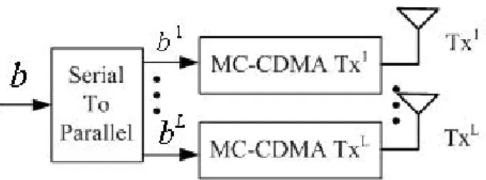
(19) Chapter 2 System Model In this chapter, the MIMO MC-CDMA system model is presented. It applies L antennas to transmit different data, so spectral efficiency becomes L times. But the layered antenna interference is also induced to the received signals. The details of system model are described and illustrated as follows.. 2.1. Transmitted Signal. Fig. 2.1: The transmitter block diagram of the MIMO MC-CDMA system. 7.

(20) The block diagram of the transmit end is shown in Fig. 2.1. The transmitted data passes through spatial multiplexing to L data streams which are delivered to L transmitters. Each data stream bl , which is called a layer, is processed by MC-CDMA transmission scheme in l Fig. 2.2. Here the data stream is mapped to QPSK symbols d k ∈ {±1 ± j} , where. 1 ≤ k ≤ K , then these symbols are modulated individually by K spreading code vectors. s k = [ sk ,1 ,… , sk ,i ,… , sk , N ]T , where. T denotes the transpose operation. After summing K. all spreading symbols, signals expressed as. ∑d s k =1. l k k. are element-wise multiplied the. l l l l T scrambling vector ξ = [ξ 1 ,… , ξi ,… , ξ N ] , which can reduce the correlation between. Fig. 2.2: The MC-CDMA transmission scheme at the lth transmit antenna. signals of different transmitters to help suppress LAI. The transmitted signal of the lth transmitter can be given by. ⎛ K l ⎞ x = ⎜ ∑ dk sk ⎟ ⎝ k =1 ⎠ l. where. denotes the element-wise product operation. 8. (2.1). ξ. l.

(21) N elements of x. l. are fed into an OFDM modulator, which includes N-point inverse. discrete Fourier transform(IFFT) block followed by a parallel to serial(P/S) block and guard interval(GI) insertion. To suppress the inter-symbol interference (ISI), the output symbols of P/S is cyclically extended with the guard interval (GI). After GI insertion, the symbol duration. T is increased to T + Tg , where the duration of GI, Tg , is equal to one-fourth of T . Then we transmit symbols at all L transmitters simultaneously.. 2.2. Received Signal. Fig. 2.3: The OFDM demodulator at the jth receive antenna. For simplification, we assume that the synchronization and channel estimation at the receivers are perfect and the maximum multipath delay spread is fewer than. Tg , so receivers. can obtain the accurate channel information and be ISI-free. The signals of all L transmitters propagate through the multipath channel and are received by M receivers. At the jth receiver, we obtain baseband signals on N subcarriers from an. 9.

(22) OFDM demodulator in Fig. 2.3. After GI deletion and FFT operation, the received signal of the jth receiver is the superposition of the signals from L transmitters plus the complex additive white Gaussian noise, given by ⎛⎛ K ⎞ r j = ∑ H j ,l ⎜ ⎜ ∑ d kl s k ⎟ ⎠ ⎝ ⎝ k =1. where. (2.2). ⎞ ξl ⎟+ Nj ⎠. T. r j = ⎡⎣ r1 j ,..., ri j ,..., rNj ⎤⎦ denotes signals on N subcarriers, H j ,l is the channel. frequency response matrix ( N × N ) between lth transmitter and jth receiver. It is defined by. H. j ,l. = d ia g { h1j , l , … , hi j , l , … , h Nj , l }. At the multipath environment, the channel matrix can be written as H. (2.3). j ,l. =. P. ∑H p =1. j ,l p. ,. where i , p and P are, respectively, the subcarrier index, the path index and the number of the paths. The N elements of N j are the complex additive white Gaussian noise with zero mean and variance σ n2 .. 10.

(23) Chapter 3 Iterative Multi-Layered Detection Methods for MIMO MC-CDMA Systems In this MIMO system, each transmitter is used to transmit different data stream that induces the layered antenna interference (LAI). The received signals which are described in Eq.(2.2) contain LAI. The data stream for individual transmitter must be detected from signals at M receivers. Each layer is considered in turn to be the desired signal, and the remainder is treated as interference. In Section 3.1, we describe the adaptive MMSE equalization for each receiver is used to suppress LAI and noise. After the equalizing and dispreading, the signals of M receivers are combined to obtain the receiver diversity, and a decision on the desired signal is made. Afterward the decision results can be used to reconstruct and cancel the received interferers from the received signals. After several iterations, the decision data is accurate enough, so we can apply the MPIC to suppress inter-code interference which results from the loss of orthogonality between spreading codes. The details of above are included in Section 3.2. By exploiting MMSE. 11.

(24) equalizer and MPIC combined with layered antenna interference cancellation (LAIC) by turn, the LAI and MPI can be reduced iteration by iteration. In Section 3.3, we present different interference cancellation orders, and the performance results are showed in section 3.4.. 3.1. Adaptive MMSE Equalizer and Iterative Layered-antenna Interference Cancellation. After process in Fig. 2.3, the MMSE equalizer for the Qth layer is applied to suppress the other layered interferers and noise at jth receiver as Fig.3.1. For the first iteration, the j ,Q equalizer factor gi is derived by minimize the mean square error between the transmitted j ,Q j Q symbol d k and the equalized signal gi ri on the ith subcarrier [18], and it can be. expressed as. g i j ,Q =. | hi j ,Q |2 +. where σ = σ + 2 K 2. 2 n. L. ∑. l =1,l ≠ Q. (3.1). (hi j ,Q )*. σ. 2. 2K. | hi j ,l |2 and K is the number of spread code used.. After the equalization, dispreading and scrambling, the signals of all M receivers is combined, then the signal of the uth spread code for the Qth layer can be expressed as. 12.

(25) ( (. M. z = ∑ suT ξ Q Q u. j =1. (G. j ,Q. rj. ))). M N M K ⎛ N ⎞ = d Qu ∑∑ gij ,Q hi j ,Q + ∑∑ d Qk ⎜ ∑ gij ,Q hi j ,Q sk ,i su ,i ⎟ j =1 i =1 j =1 k=1 ⎝ i =1 ⎠ k≠u. Desired Signal. Inter-code Interference. M N ⎛ N j ,Q j ,l Q l ⎞ + ∑ ∑ ∑ d ⎜ ∑ gi hi sk ,i su ,iξi ξi ⎟ + ∑∑ su ,i gij ,Q nijξiQ j =1 l =1,l ≠ Q k=1 ⎝ i =1 ⎠ j =1 i =1 M. L. K. l k. Layered Antenna Interference. where G. j ,Q. (3.2). Enhanced Noise. = diag { g 1j , Q , … , g i j , Q , … , g Nj ,Q } . The spreading chips are transmitted. through multiple carriers over the frequency selective channel that causes the equivalent j ,Q. channel gain which equals gi hi. j ,Q. is not the same on N chips and the orthogonality. between spreading codes is destroyed. Hence, the inter-code interference (ICI) is induced. In addition to ICI, layered antenna interference and enhanced noise are also the reasons for the performance degradation. Q l After the decision is made on zu , the decision results dˆ k are delivered to the next. iteration. The layered antenna interference cancellation scheme which combines with MMSE l equalization is illustrated in Fig. 3.2. The decision result dˆ k passes through spreading,. scrambling and multiplying channel gain hi j ,l to reconstruct the interference from other transmitters. The LAI is subtracted from the received signal. ⎛⎛ K ⎞ ˆr j ,Q = r j − ∑ H j ,l ⎜ ⎜ ∑ dˆkl s k ⎟ l∈I ⎠ ⎝ ⎝ k =1. ⎞. r j , then we have (3.3). ξl ⎟ ⎠. 13.

(26) 14. Fig.3.1:The first iteration of multilayered detection method.

(27) where I includes the transmitter index which we want to cancel, and Q is not included. Because some LAI are cancelled from adjusted to σ 2 = σ n2 + 2 K. L. ∑. l =1,l∉I,l ≠ Q. r j , the coefficient of MMSE equalizer in Eq.(3.1) is. | hi j ,l | , and the signal before decision can be expressed as. follows:. ( (. M. (G. zˆ = ∑ suT ξ Q Q u. j =1. M. =d. Q u. N. ∑∑ g j =1 i =1. j ,Q i. hi. j ,Q. j ,Q. rˆ j. ))). ⎛ N j ,Q j ,Q ⎞ + ∑∑ d ⎜ ∑ gi hi sk ,i su ,i ⎟ j =1 k=1 ⎝ i =1 ⎠ M. K. Q k. k≠u. Desired Signal. Inter-code Interference. ⎛ ⎞ + ∑∑∑ (d lk − dˆ lk ) ⎜ ∑ gij ,Q hi j ,l sk ,i su ,iξiQξil ⎟ j =1 l∈I k=1 ⎝ i =1 ⎠ M. K. N. (3.4). Residual Layered Antenna Interference. ⎛ N j , Q j ,l ⎞ + ∑ ∑ ∑ d ⎜ ∑ gi hi sk ,i su ,iξiQξil ⎟ j =1 l =1,l∉I ,l ≠ Q k=1 ⎝ i =1 ⎠ M. L. K. l k. Layered Antenna Interference M. N. + ∑∑ su ,i gij ,Q nijξiQ j =1 i =1. Enhanced Noise l where the residual LAI is due to the decision errors for other layers. If the decision result dˆ k. is correct, the residual LAI from the lth transmitter will be cancelled, such that the decision for Qth layer becomes more accurate and some decision errors made before will be corrected. Theoretically, the LAI cancelled in later iteration will be more accurate than the former, and this system is finally free of LAI. In practice, however, the error propagation may occur between layers because the interference is so serious at first that decision results have. 15.

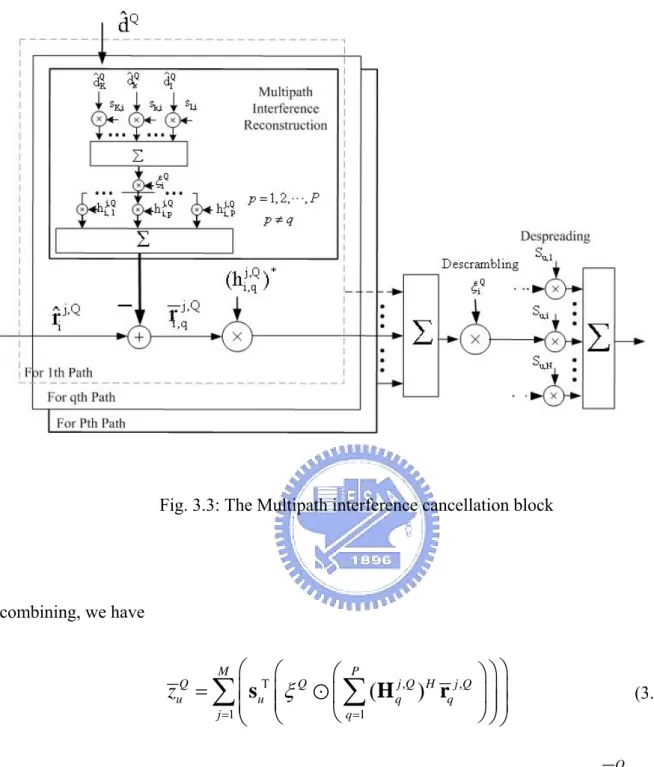
(28) too many errors.. Multipath Interference Cancellation. 3.2. As described in Eq.(3.2), inter-code interference which comes from the loss of orthogonality between spreading codes is one of the reasons for the performance degradation. If each path is matched individually, the frequency response will become flat to avoid ICI, and the multipath diversity can be obtained additionally. Thus when the decision data is accurate enough, we use the multipath interference cancellation (MPIC) scheme following MMSE equalization as Fig. 3.2.. The details of the MPIC block are illustrated in Fig. 3.3. For the qth path, the interferers from other paths ( p = 1 ~ P, p ≠ q ) for the Qth layer are reconstructed and cancelled from rˆ j ,Q which has cancelled LAI, so it can be expressed as. rq. j ,Q. = rˆ. j ,Q. −. P. ∑. p =1, p ≠ q. H. j ,Q p. ⎛ ⎛ K ˆQ ⎞ ⎜ ⎜ ∑ dk sk ⎟ ⎠ ⎝ ⎝ k =1. ⎞ ξ ⎟ ⎠. (3.5). Q. j ,Q Afterward maximum ratio combining is exploited to get multipath diversity gain. rq is. matched by the complex conjugate of the channel frequency response for the qth path, and the sum of all matched signals is descrambled and despread. After receiver diversity. 16.

(29) 17. Fig. 3.2: The second and subsequent iterations of multilayered iteration method.

(30) Fig. 3.3: The Multipath interference cancellation block. combining, we have. ⎛ ⎛ z = ∑ ⎜ suT ⎜ ξ Q ⎜ ⎜ j =1 ⎝ ⎝ M. Q u. ⎛ P ⎞⎞⎞ j ,Q H j ,Q ( H ) r ⎜∑ q ⎟ ⎟⎟ ⎟⎟ q ⎝ q =1 ⎠⎠⎠. where ( i ) H denotes the conjugate transpose operator. Then the decision is made on. (3.6). zuQ .. After several iterations, the LAI is almost cleared and the MMSE equalization can’t improve performance any more, so we remove the MMSE equalization and only apply MPIC at subsequent iterations.. 18.

(31) 3.3. Successive and Parallel Interference Cancellation. The successive interference cancellation (SIC) scheme, as its name, detects L layers successively. The decision results from the former layers are exploited to cancel LAI or MPI for the later. Hence, for the first iteration, LAIC has been employed as shown in Fig. 3.2, and the set of recostructed layers I for the Qth layer in Eq.(3.3) includes Q-1 layers which have been detected before. For the later layer detection, signals will have less interference and more accurate decision results. Thus the iteration denotes that all layers finish detecting sequentially. After the second iteration, the set I includes all layers except the Qth layer.. In contrast, the parallel interference cancellation (PIC) scheme detects all layers simultaneously. The set I is null for the first iteration, and includes all layers except the Qth layer for the following iterations. For the PIC architecture, the iteration denotes that all. layers finish detecting simultaneously. Thus LAI has never been deleted from received signals will make more decision errors than SIC, then incorrect LAI cancellation for the following iteration is induced by these errors that degrades the performance, and even serious error propagation occurs between layers. Although PIC spends less time for each iteration, SIC may obtain better performance finally. The performance comparison of these methods is illustrated and discussed in Section 3.4.1.. 19.

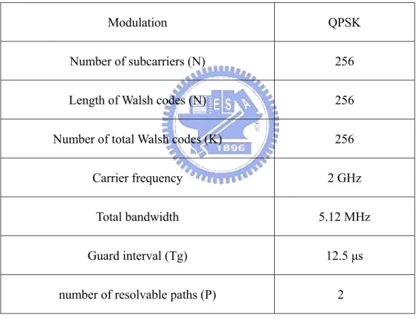
(32) 3.4 Performance Results We compare the performance of iterative multi-layered detection methods with different interference cancellation architectures and different numbers of spread code used in this section. Additionally, these methods are also compared with VBLAST at their performance and computation complexity.. Modulation. QPSK. Number of subcarriers (N). 256. Length of Walsh codes (N). 256. Number of total Walsh codes (K). 256. Carrier frequency. 2 GHz. Total bandwidth. 5.12 MHz. Guard interval (Tg). 12.5 μs. number of resolvable paths (P). 2. Table 3.1:Simulation parameters. The simulation parameters are listed in Table 3.1. We apply the Walsh code to spread symbols and a pseudo random code generator to produce the scrambling codes. It is assumed that synchronization and channel estimation are perfect, and the noise power is known at the 20.

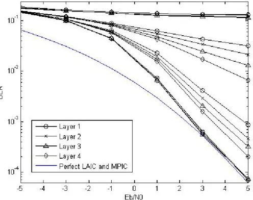
(33) receive end. The equivalent baseband impulse response of the multipath fading channel between lth transmitter and jth receiver is modeled by P. (3.7). ϕ (t ) = ∑ a δ (t − τ ) j ,l. p =1. j ,l p. j ,l p. where a pj ,l and τ pj ,l are, respectively, the complex amplitude and excess delays of pth multipath component. P denotes the number of resolvable paths and δ (•) is the unit impulse function. In our simulations, τ pj ,l is uniformly distributed between 0 μ s to 12.5 μ s , a pj ,l is generated by complex Gaussian random variable, and for the two-path channel model, the power ratio of paths is 0:0 (dB). Furthermore, the fading patterns of each path between each transmitter and receiver are generated independently. Throughout this chapter, the process procedure is presented in Table 3.2. iteration. 1st. 2nd~4th. 5th~9th. process. MMSE. MMSE and MPIC. MPIC. Table 3.2: The process procedure. 3.4.1. The Performance Comparison with Different Interference Cancellation Architectures. The BER performance of the MIMO system with four transmitters and four receivers using successive interference cancellation is showed in Fig. 3.4. At early iterations, we observe that the layer detected later always has better performance. However, when the information of all layers is propagated adequately at later iterations, all layers will have the 21.

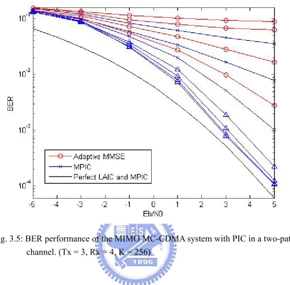
(34) same performance. We can find the BER at high Eb/N0 is close to the performance with perfect LAIC and MPIC, the bound of diversity order equals to 8. By exploiting this detection method with SIC in MIMO system, the spectral efficiency becomes eight times in SISO system.. Fig. 3.4: BER performance of the MIMO MC-CDMA system with SIC for all four layers in a two-path channel at iteration 1, 3, 5 and 9. (Tx = 4, Rx = 4, K = 256). 22.

(35) Fig. 3.5: BER performance of the MIMO MC-CDMA system with PIC in a two-path channel. (Tx = 3, Rx = 4, K = 256). From the simulation results of the system (Tx = 4, Rx = 4) with PIC architecture, we find that the error propagation occurs, so the iterative interference cancellation can’t improve the performance. Fig. 3.5 shows the performance of the system which decreases the number of transmitter to three. We observe that the speed of convergence is almost the same as that of the system with SIC. Hence, the spectral efficiency of the PIC architecture is three-fourths of SIC. But the former spends lesser process time than the later.. 23.

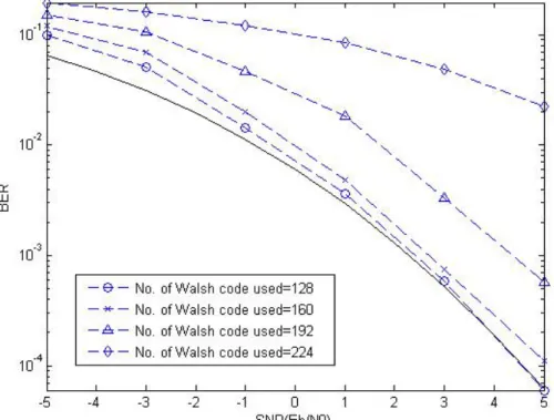
(36) 3.4.2. Effect of the Number of Walsh Codes Used. The number of Walsh codes used (K) will affect the LAI, ICI and spectral efficiency. Fig. 3.6 shows the effect of the number of Walsh codes used. In this MIMO MC-CDMA system (Tx = 4, Rx = 4) using PIC, We can find that more Walsh codes are used, more LAI and ICI occur to received signals. Thus, the performance of the system which uses fewer Walsh codes is more close to the theoretical performance, but its spectral efficiency is lower. We compare it with the system using PIC described in section 3.4.1, the highest spectral efficiency of these workable systems, 5 bits/sec/Hz, is still lower slightly than that of the system with PIC using three transmitters, 6 bits/sec/Hz.. 24.

(37) Fig. 3.6: BER performance of the MIMO MC-CDMA system with PIC versus the number of Walsh codes used in a two-path channel. (Tx = 4, Rx = 4). 25.

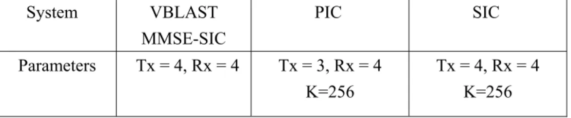
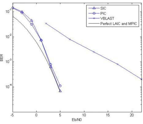
(38) 3.4.3. The Performance Comparison between V-BLAST and the Proposed Systems. Fig. 3.7 shows the BER performance comparison between VBLAST and the proposed systems. The system parameters are showed in Table 3.3.. System. VBLAST MMSE-SIC. PIC. SIC. Parameters. Tx = 4, Rx = 4. Tx = 3, Rx = 4 K=256. Tx = 4, Rx = 4 K=256. Table 3.3: The system parameters of VBLAST and the proposed systems.. Here we use the VBLAST with the MMSE detector and successive interference cancellation in OFDM system to compare with our proposed methods. The performance of VBLAST is far away from the theoretical bound and our systems. In the Multipath channel, the frequency selective effect will make the symbols on some carriers fade seriously in the OFDM system. If the symbols are spread to all subcarriers, as in MC-CDMA, the effect will be mitigated. Our proposed methods exploit MC-CDMA system to increase frequency diversity and resist the frequency selective fading. MPIC is applied to combine the multipath diversity gain that VBLAST can’t obtain. Our proposed systems can achieve the performance of perfect LAIC and MPIC. But the system with parallel interference cancellation has lower spectral efficiency than the other systems.. 26.

(39) The complexity comparison between them is presented in Table 3.4. Most complexity of our proposed systems is used on spreading and despreading process. The complexity of the PIC is lower than SIC in the first iteration, and both of them are much higher than V-BLAST. We can compare PIC architecture with the layered space-time (LST) technique mentioned in [4]. Although the LST technique combines layered space time scheme and turbo coding, the performance are still worse than our proposed systems.. Fig. 3.7: BER performance comparison between VBLAST and the proposed systems in a two-path fading channel.. 27.

(40) Architecture. Process. SIC. PIC. V-BLAST. ( L’= number of elements in I , L = 4, M= 4). ( L’= number of elements in I , L = 3, M = 4 ). ( L’= number of residual layers, L= 4, M = 4) each layer at all receivers. Each layer at each receiver 2 L ' NK + 6 NL '. LAIC. 2 L ' NK + 6 NL '. 4 NML '. MMSE. 8 N + 2 KN + 2. 4 N (2ML '2 + L '3 ). MPIC. 8 NP + 2 N ( K + 1). 0. All L layers at M receivers / the average for each layer at M receivers 1st iteration. 3721248 / 930312. 1597464 / 532488. 360448 / 90112. LAIC+MMSE. 6422560 / 1605640. 4816920 / 1605640. 802816 / 200704. +MPIC iteration LAIC+MPIC iteration. (for the other iterations) 4292608 / 1073152. 3219456 / 1073152. Table 3.4: The complexity comparison of multi-layered detection methods ( measured by the number of the real multiplier, N=256, K=256 , P=2. ).. 28.

(41) Chapter 4 Parallel Iterative Multi-Layered Detection Method for Bit-Interleaved Coded Modulation in MIMO MC-CDMA Systems. Here we describe a parallel iterative multi-layered detection method which combines soft interference cancellation, adaptive MMSE detector and bit-interleaved coded modulation (BICM). By exploiting soft information from output of the soft-in soft-out decoder at receive end, the interference reconstruction is more reliable, so the situation of the error propagation is reduced. The bits which are affected by the same channel gain or correlate with each other are spread by the bit interleavers to resist bursty errors induced by the correlated fading and maximize the diversity order.. In the Section 4.1, we present the BICM scheme proposed in [15]. Our proposed method is presented in the Section 4.2, and the simulation results are included in the last section.. 29.

(42) 4.1. 4.1.1. Bit-Interleaved Coded Modulation The Transmitter. Fig. 4.1: The transmitter block diagram of the 8PSK bit-interleaved coded modulation.. The BICM transmitter is showed in Fig. 4.1, where t is the time index. The BICM transmitter is a serial concatenation of the convolutional encoder, the interleaver and the 8-PSK modulator. Here we use a rate-2/3 convolutional encoder, a group of independent bit interleavers and an 8-PSK modulator. By applying 8-PSK modulation, the bandwidth efficiency is not lost on coding. At first two data bits bt = [b0t ,b1t ] are encoded to three bits Ct =[C0t , C1t ,C2t ] , and Ct passes through the interleaver which is the combination of three bit interleavers. In order to mitigate bursty errors and maximize the diversity order, the interleaver design can follow some rules below :. z. Using three independent interleavers to ensure the coded bits with different protection 30.

(43) keep their different positions at the symbol labeling.. z. The interleaved coded bits Vt =[Vt0 , Vt1 ,Vt2 ] modulated to the same symbol must come from Cit which are at a distance larger than the code constraint length from each other.. z. The coded bits close to each other at code trellis will be modulated to symbols which apart from each other or suffer uncorrelated channel gains. After interleaving, Vt is mapped to a 8-PSK symbol by a mapping operator μ . The. symbol d t belongs to Ω , the 8-PSK constellation, and is transmitted. d t =μ ([Vt0 ,Vt1 ,Vt2 ]) , d t ∈ Ω. 4.1.2. (4.1). The Receiver. Fig. 4.2: The receiver block diagram of the 8PSK bit-interleaved coded modulation.. The receive signal can be presented as y t = H × d t + n , where H is the channel gain and n is the complex additive white Gaussian noise. The BICM receiver block diagram is showed in 31.

(44) Fig. 4.2. Here we use the suboptimal method with separate steps, demapper and decoder. They are separated by bit interleavers used to return the coded bit information to original sequence. The details of the demapper and soft-in soft-out decoder are described below:. a. Demapper This block is used to demodulate channel symbol and obtain bit information for decoding. The bit information is computed by using the maximum a-posterior probability criterion. The a-posteriori probability of coded bit can be calculated as. p(Vti = c | yt ) =. ∑. w∈Ωic. p ( w | yt ) =. {. }. where Ωic = μ ([Vt0 ,Vt1 ,Vt2 ]) | Vti = c. ∑. w∈Ωic. p( yt | w) p ( w) p ( yt ). (4.2). is a subset of 8-PSK constellation whose size is four,. c= 0 or 1 and w is a 8-PSK symbol. For the fading channel, the conditional probability of received signal can be presented as the complex Gaussian distribution. p ( yt | w) =. 1 2πσ. e 2. −. | yt − H t w|2 2σ 2. (4.3). where σ 2 is the noise variance. We use the log likelihood ratio (LLR) to deal with the bit information. The a-posterior LLR of coded bit is defined as ⎛ p (Vti = 0 | yt ) ⎞ Λ (Vti | yt ) = ln ⎜ ⎟ i ⎝ p (Vt = 1| yt ) ⎠. (4.4). Substituting Eq.(4.2) into Eq.(4.4) and assuming independent bits (using the random enough 32.

(45) interleavers), we have 2 ⎛ ⎞ ⎛ ⎞ p ( y | w ) p ( w ) p ( y | w ) pa (Vti' = V i' ( w)) ⎟ ∏ t t ⎜ ∑ ⎜ ∑ ⎟ i'=0 w∈Ωi0 ⎟ ⎟ = ln ⎜ w∈Ωi0 Λ (Vti | yt ) = ln ⎜ 2 ⎜ ⎟ ⎜ ⎟ i' i' ⎜ ∑ p( yt | w)∏ pa (Vt = V ( w)) ⎟ ⎜ ∑ p( yt | w) p( w) ⎟ ⎜ w∈Ωi ⎟ ⎜ w∈Ωi ⎟ i'=0 1 1 ⎝ ⎠ ⎝ ⎠. (4.5). where V i' ( w) ∈ {0,1} denotes the value of the i’th bit for the symbol w .. The a-priori LLR of Vti is defined as. , thus we can obtain. pa (Vti = c) =. ⎛ p (V i = 0) ⎞ Λ a (Vti ) = ln ⎜ a ti ⎟ ⎝ pa (Vt = 1) ⎠. exp{-Λ a (Vti ) × c} , for c = 0 or 1 1 + exp{-Λ a (Vti )}. (4.6) (4.7). Substituting Eq.(4.3) and Eq (4.7) into Eq.(4.5), we have | y − H w|2 2 ⎛ ⎞ − t 2t exp{-Λ a (Vti' ) × V i' ( w)} ⎟ 1 σ 2 ⎜ ∑ e ∏ ⎜ w∈Ωi 2πσ 2 1 + exp{-Λ a (Vti' )} ⎟ i'=0 i 0 Λ (Vt | yt ) = ln ⎜ ⎟ | y − H w|2 2 i' i' − t 2t ⎜ ⎟ exp{(V ) V ( w )} Λ × 1 t a e 2σ ∏ ⎜ ∑ ⎟ 2 i' ⎜ w∈Ωi 2πσ 1 + exp{-Λ a (Vt )} ⎟ i'=0 1 ⎝ ⎠ ⎛ ⎞ | yt − H t w |2 2 − ∑ Λ a (Vti' ) × V i' ( w)} ⎟ ⎜ ∑ exp{− 2 2σ i'=0 w∈Ωi0 ⎟ = ln ⎜⎜ 2 2 ⎟ | y − Ht w | i' i' (V ) V ( w )} − Λ × ⎜ ∑ exp{− t ⎟ ∑ t a ⎜ w∈Ωi ⎟ 2σ 2 i'=0 1 ⎝ ⎠. (4.8). The a-posterior LLR of the coded bit can also be written as. ⎛ p( yt | Vti = 0) ⎞ ⎛ p(Vti = 0) ⎞ ln Λ(Vti | yt ) = ln ⎜ + ⎟ ⎜ ⎟ i i ⎝ p( yt | Vt = 1) ⎠ ⎝ p(Vt = 1) ⎠ extrinsic information. ⎛ | yt ⎜ ∑ exp{− w∈Ωi0 = ln ⎜⎜ |y ⎜ ∑ exp{− t ⎜ w∈Ωi 1 ⎝. a-priori probability 2 ⎞ − H t w |2 − Λ a (Vti ' ) × Vi ' ( w)} ⎟ ∑ 2 2σ i '= 0,i '≠ i ⎟ + Λ (Vi ) a t 2 2 ⎟ − Ht w | i' i' − Λ × w (V ) V ( )} ⎟ ∑ a t ⎟ 2σ 2 i '= 0,i '≠ i ⎠. 33. (4.9).

(46) The extrinsic information term output by the demapper is ⎛ | yt ⎜ ∑ exp{− w∈Ωi0 Λ ex (Vti ) = ln ⎜⎜ |y ⎜ ∑ exp{− t ⎜ w∈Ωi 1 ⎝. 2 ⎞ − H t w |2 − Λ a (Vti ' ) × Vi ' ( w)} ⎟ ∑ 2 2σ i '= 0,i '≠ i ⎟ 2 2 ⎟ − Ht w | i' i' (V ) V ( w )} − Λ × ⎟ ∑ a t ⎟ 2σ 2 i '= 0,i '≠ i ⎠. (4.10). where the a-priori information Λ a (Vti ' ) comes from the output of the decoder in Fig. 4.2. Because Λ a (Vti ' ) is not available at the first demapping, we assume it is equally likely, and Eq.(4.10) becomes ⎛ | yt ⎜ ∑ exp{− w∈Ωi0 Λ ex (Vti ) = ln ⎜⎜ |y ⎜ ∑ exp{− t ⎜ w∈Ωi 1 ⎝. − H t w |2 ⎞ ⎟ 2σ 2 ⎟ − H t w |2 ⎟ ⎟ ⎟ 2σ 2 ⎠. (4.11). Then Λ ex (Vti ) is deinterleaved and sent to the decoder. After the first decoding, the extrinsic information of coded bits Λ ex (Cit ) is delivered by the decoder to the interleaver and becomes Λ a (Vti ) , the a-prior probability of the demapper. The process to exchange information between demapper and decoder is continued, and the final decoding output is the a-posteriori information of data bits Λ ex (bit ) , i = 0 or 1.. 34.

(47) a. Gray Labeling. b. Set-Partitioning Labeling Fig. 4.3: Two signal labeling schemes, the bits from left to right are Vt0 , Vt1 and Vt2 .. The improvement of iterative demapping is much-correlated with the signal labeling. Two general signal labeling schemes are showed in Fig. 4.3. For the ith bit, the subset Ω1i includes the symbols in the shadow regions, and the other symbols are included in Ωi0 are in the white regions. In the figure of the ith bit, the pair of symbols which have the same bits except the ith bit is connected by a line. When we use the a-prior information of the other bits ( ≠ Vti ) from interleaver to help demap Vti , one of four pairs is chosen and 8-PSK mapping is 35.

(48) translated to binary modulation. Because of the reduction of the nearest neighbor symbols, the distance between the symbols in the pair becomes larger and the extrinsic information of the ith bit Λ ex (Vti ) is more reliable. Thus the improvement of iterative detection is much relative to the signal labeling scheme used.. Comparing two signal labeling schemes, the average distance of all pairs of symbols in set-partition labeling is larger than Gray labeling, so set-partition labeling has better improvement with iterative decoding. However, Gray labeling have fewer nearest neighbor symbols in the beginning because the neighbor symbols for every symbol are only different in one bit. Hence it will provide more reliable soft information for the first iteration than set-partition labeling. For the MIMO systems, layered antenna interference is so serious that if the set-partition labeling scheme is used, the extrinsic information of the demapper for the first iteration will be unreliable. The terrible information is passed between the demapper and decoder for the following iterations and error propagation occurs. That is the reason why we use Gray labeling scheme for our proposed iterative multi-layered method presented in this chapter.. B. Soft-in soft-out decoder After deinterleaving the output of the demapper, Λ a (Cit ) is utilized to decode. Here we. 36.

(49) use the soft-in soft-out decoder which applies the modification of BCJR algorithm suggested by [17]. This algorithm defines the forward and backward recursions as follows: (4.12). 2 ⎛ ⎞ α t ( s ) = ∑ ⎜ α t −1 ( s ')∏ Pa {Ci't = Ci' (s, s ')} ⎟, all s' ⎝ i'=0 ⎠. ⎛. 2. ⎞. ⎝. i'=0. ⎠. t=1,2,… ,τ. β t (s) = ∑ ⎜ βt +1 ( s ')∏ Pa {Ci't+1 = Ci' (s ', s)} ⎟, all s'. The boundary conditions:. (4.13). t=τ -1,τ -2,… ,0. α 0 ( s = 0) = 1 α 0 (s ≠ 0) = 0. And. βτ ( s = 0) = 1 βτ (s ≠ 0) = 0. where Ci' ( s, s ') denotes the jth coded bit for the state transition (s,s’), τ is the length of coding sequence, and the summation is over all s ' which make the state transition ( s, s ') possible. Compare with BCJR algorithm, α t (s) and β t ( s) are, respectively, the forward and backward probability for the state s at time t. The probability of the state transition ( s, s ') at time t, γ t ( s, s ') , is substituted by the product of the probability of the coded bits which come from the demapping output. For simplification, we use the natural logarithm of the probability, α t and β t , intead of the probability to express the forward and backward recursions, where α t =ln(α t ) and. β t = ln( βt ) . Besides, pa (Cit ) can be derived like Eq.(4.7) exp{-Λ a (Cit ) × c} pa (C = c) = , for c = 0 or 1 1 + exp{-Λ a (Cit )}. (4.14). i t. where Λ a (Cit ) comes from the deinterleaver output. Substitute it into Eq.(4.12) and 37.

(50) Eq.(4.13), we have ⎛. 2. ⎞. ⎝. i '= 0. ⎠. α t (s) = ln ∑ exp ⎜ α t −1 (s') + ∑ (−Λ a (Cit ' ) × Ci ' (s',s)) ⎟ , t=1,2,… ,τ all s'. ⎛. 2. ⎞. ⎝. i '= 0. ⎠. βt (s) = ln ∑ exp ⎜ β t +1 (s') + ∑ (−Λ a (Ci't+1 ) × Ci' (s,s')) ⎟ , t=τ -1,τ -2,...,0 all s'. (4.16). (4.15). and the denominator in Eq.(4.14) is normalized for all α t (s t ) and β t (s t ) . Define ϒi0 and ϒ1i are the set of state transitions ( s ', s ) such that the ith coded bit is, respectively, 0 and 1. The a-posteriori LLR of the coded bit Cit at the output of the decoder is given by ⎧. 2 ⎫ (s') + β t (s) − ∑ Λ a (Cit ' ) × Ci ' (s',s) ⎬ i '= 0 ⎭ ϒ0 Λ (Cit )=ln i 2 ⎧ ⎫ Λ a (Cit ' ) × Ci ' (s',s) ⎬ ∑1 exp ⎨⎩α t −1 (s') + βt (s) − ∑ i '= 0 ⎭ ϒi. ∑ exp ⎨⎩α. t −1. ⎧. (4.17). ⎫ Λ a (Cit ' ) × Ci ' (s',s) ⎬ i '= 0,i '≠ i ϒ0 ⎩ ⎭ = ln i 2 ⎧ ⎫ Λ a (Cit ' ) × Ci ' (s',s) ⎬ ∑1 exp ⎨α t −1 (s') + βt (s) − i '=∑ 0,i '≠ i ϒi ⎩ ⎭. ∑ exp ⎨α. t −1. (s') + β t (s) −. 2. ∑. Λex (Cti ). +Λ a (Cit ). It’s the summation of the extrinsic information Λ ex (Cik ) and a-priori information Λ a (Cik ) . Λ ex (Cik ) is obtained from the a-prior information of the other coded bits by the trellis structure of the code, and Λ a (Cik ) is supplied by the deinterleaver output. The extrinsic information Λ ex (Cik ) is what the decoder sends to help demap for the following iterations. We can also compute the a-posteriori LLR of the data bits for the final decoding results.. 38.

(51) Similarly, define Γi0 and Γ1i are the set of state transitions ( s ', s) such that the ith data bit bit is, respectively, 0 and 1. The a-posteriori LLR of the data bit is given by ⎧. 2 ⎫ (s') + βt (s) − ∑ Λ a (Cit ' ) × Ci ' (s',s) ⎬ i '= 0 ⎭ Γ0 Λ (bit )=ln i 2 ⎧ ⎫ Λ a (Cit ' ) × Ci ' (s',s) ⎬ ∑1 exp ⎩⎨α t −1 (s') + βt (s) − ∑ i '= 0 ⎭ Γi. ∑ exp ⎩⎨α. t −1. (. ). (. ). (4.18). Finally, the decision is made on Λ (bit ) . If Λ (bit ) is larger than 0, the decision result of bit will be 0, or 1 otherwise.. 39.

(52) 4.2. Transmit End of the MIMO MC-CDMA System with BICM. The block diagram of the transmit end is showed in Fig. 4.4. The coding scheme which concatenates the convolutional encoder, interleaver and mapper is used to preprocess the data bits bit before spatial multiplexing. The interleaver is a parallel connection of three independent bit interleavers, and the length of each bit interleaver is equal to the number of symbols in a transmitted block, a multiple of L × K . After Gray labeling mapping, the 8-PSK symbols are spatially multiplexed to L symbol streams which are delivered to L transmitters.. Fig. 4.4: The transmitter block diagram of the MIMO MC-CDMA system. Fig. 4.5: The scheme diagram of the lth MC-CDMA transmitter. 40.

(53) The scheme diagram of the lth MC-CDMA transmitter is showed in Fig. 4.5. The only difference of the systems between Fig. 4.5 and Fig. 2.2 is that the input here is the 8-PSK symbol streams and the QPSK modulator is taken away, thus we can express transmit signals here as in Section 2.1. The symbol streams are processed by multiplexing to K symbol stream and spread by individual spread codes. After summing, serial-to-parallel and scrambling, the signal can be expressed as. K. x = ∑d s l. k =1. l k k. ξ. (4.19) l. After being modulated to the OFDM symbosls and inserting GI, all signals at L transmitters are transmitted simultaneously.. 4.3. Parallel Iterative Multi-Layered Detection Method. 4.3.1. Receive Signal. The signals transmitted by all L transmitters propagate through the multipath channel and are received by M receivers. As described in Section 2.2, the baseband signals at jth receiver which are obtained by the OFDM demodulator in Fig. 2.3 can be expressed as 41.

(54) ⎛⎛ K ⎞ r = ∑ H ⎜ ⎜ ∑ d kl s k ⎟ l =1 ⎠ ⎝ ⎝ k =1 L. j. j ,l. ⎞ ξ ⎟+Nj ⎠. (4.20). l. where these symbols, r j , H j ,l and N j , have the same meanings as mentioned in Section 2.2.. 4.3.2. Overview on the Parallel Iterative Multi-layered Detection Method. The parallel multi-layered detection method exploits the soft information instead of hard decision results to implement adaptive MMSE equalization, MPIC and LAIC, thus the information of layered detection and decoding can be passed to each other and exchanged between layers adequately. For the reason of saving process time, we adopt parallel interference cancellation architecture in our proposed method.. The scheme diagram for the first iteration is shown in Fig.4.6. After OFDM demodulation, the baseband signal at jth receiver, r j , passes through MMSE equalizer to suppress layered-antenna interference and noise. After being despread, scrambled and summed up for all L receivers to combine receiver diversity, the signal is delivered to the BICM decoder block.. In the decoder block, the signal is demapped to the information of three coded bits firstly,. 42.

(55) 43. Fig.4.6: The first iteration of the multilayered detection method..

(56) and the bit deinterleavers are used to return the information to the encoding order. After iteratively decoding and demapping, the a-posteriori information of coded bits will be obtained from the output of the decoder and be exploited to generate the soft symbol.. For the following iteration, the soft symbols of the previous iterations are utilized to reconstruct and cancel LAI. The soft symbol can also be exploited to adjust the factors of adaptive MMSE equalizer and calculate the statistics of signals to help demap. The block diagram is illustrated in Fig. 4.7.. Through several iterations, the soft symbols become more and more reliable, we can replace the MMSE equalizer by the MPIC scheme shown Fig. 3.3. After LAIC, MPIC exploits soft symbols to reconstruct and delete MPI, and matches each path individually to suppress intercode interference (ICI) and combine multipath diversity. The block diagram of the iteration with MPIC is shown in Fig. 4.8. The details of adaptive MMSE equalizer, MPIC, symbol demapper and soft symbol block are described as follows:. A. Adaptive MMSE equalizer. For the first iteration, because the soft information of the transmit symbols is not available, we use the factor derived in Eq.(3.1) to equalize r j . Thus the signal before demapping in Fig.4.6 can be expressed as. 44.

(57) 45. Fig. 4.7: The second iteration of the multilayered detection method..

(58) 46. Fig. 4.8: The MPIC iteration of the multilayered detection method..

(59) ( (ξ. M. z =∑ s Q u. j =1. M. =d. Q u. T u. N. ∑∑ g j =1 i =1. (G. Q. j ,Q i. hi. j ,Q. j ,Q. r. j. (4.21). ))). ⎛ N j ,Q j ,Q ⎞ + ∑∑ d ⎜ ∑ gi hi sk ,i su ,i ⎟ j =1 k=1 ⎝ i =1 ⎠ M. K. Q k. k≠u. Desired Signal. Inter-code Interference. M N ⎛ j ,Q j ,l Q l ⎞ + ∑ ∑ ∑ d ⎜ ∑ gi hi sk ,i su ,iξi ξi ⎟ + ∑∑ su ,i gij ,Q nijξiQ j =1 l =1,l ≠ Q k=1 ⎝ i =1 ⎠ j =1 i =1 M. L. N. K. l k. Layered Antenna Interference. Enhanced Noise. where G j ,Q is a diagonal matrix to represent the equalization, and its ith element is. g i j ,Q =. Where σ 2 = σ n2 + 2 K. L. ∑. l =1,l ≠ Q. (hi j ,Q )* | hi j ,Q |2 +. (4.22). σ2. 2K. | hi j ,l |2 , K is the number of spread code used and σ n2 is the noise. power.. Assuming transmitted symbols are independent to each other, zuQ can be model as a complex Gaussian distribution from the central limit theorem. It consists of four components: the desired signal (DS), the inter-code interference (ICI), the layered antenna interference (LAI) and the enhanced noise (EN).The mean of the distribution comes from the DS term, and the variance comes from the other terms. Here we use h eq to represent the equivalent channel gain for the desired signal. The means of the real part Re{zuQ } and the imaginary part Im{zuQ } can be obtained. M. N. μ zI = E[Re{zuQ }] = Re{d Qu }∑∑ gij ,Q hi j ,Q j =1 i =1. 47. (4.23).

(60) M. (4.24). N. μ zQ = E[Im{zuQ }] = Im{d Qu }∑∑ gij ,Q hi j ,Q j =1 i =1. Thus h eq for the iteration with MMSE equalizer is a real number. M. N. ∑∑ g j =1 i =1. j ,Q i. hi j ,Q . The ICI is. induced by the frequency selective channel effect, thus the variance of ICI is M. (4.25). N. Var[ICI]=(K-1)E av ∑∑ | ψ i j ,Q |2 j =1 i =1. where ψ i j ,Q = gij ,Q hi j ,Q −. 1 N. N. ∑g i =1. j ,Q i. hi j ,Q , the equivalent channel gain of the ith subcarrier which. deletes the common part for all N subcarriers, E av denotes the power of 8-PSK symbol.. The variance of LAI and EN are, respectively, calculated as. M. Var[LAI]=K ⋅ E av ∑. L. ∑ ∑| g. j =1 l =1,l ≠ Q i =1. Var[EN]=σ. 2 n. M. j =1 i =1. j ,Q i. j ,l 2. hi |. (4.27). N. ∑∑ | g. (4.26). N. j ,Q 2 i. |. Hence the variances of Re{zuQ } and Im{zuQ } are given by. 1 2. σ z2 =Var[Re{zuQ }] = Var[Im{zuQ }]= ( Var[ICI]+ Var[LAI]+ Var[EN]). (4.28). Afterward the mean and variance of zuQ are applied in the demapper block. For the second and following iteration, the soft symbols dˆ l are supplied, and LAIC can be applied. At the left of Fig. 4.7, the receive signal which has deleted LAI can be presented as. 48.

(61) K ⎞ j ,l ⎛ ⎛ l l ⎞ H ⎜ ⎜ ∑ dk sk ⎟ ξ ⎟ ∑ l =1,l ≠ Q ⎠ ⎝ ⎝ k =1 ⎠ L ⎛⎛ K ⎞ ⎛⎛ K ⎞ ⎞ =H j ,Q ⎜ ⎜ ∑ d kQs k ⎟ ξ Q ⎟ + ∑ H j ,l ⎜ ⎜ ∑ (d kl − dˆkl )s k ⎟ ⎠ ⎠ ⎝ ⎝ k =1 ⎠ l =1,l ≠Q ⎝ ⎝ k =1 L. rˆ j ,Q = r j −. (4.29). ⎞. ξl ⎟+ Nj ⎠. Where dˆkl is the soft symbol with the kth spread code for the lth layer. The subtracted term is produced by LAI reconstruction block in the top of Fig. 4.7. Then the adaptive equalizer parameter σ 2 in Eq.(4.22) is adjusted to L. ∑. σ =σ + 2. 2 n. l =1,l ≠ Q. j ,l 2. | hi |. K. ∑ E[| d k =1. − dˆkl |2 ]. l k. (4.30). where E[•] is the average operator for the transmitted symbol. Because the soft symbol dˆkl is the mean of the transmitted symbol d kl and the mean of the 8-PSK symbol power is 1, it can be rewritten as L. ∑. σ =σ + 2. 2 n. l =1,l ≠ Q L. =σ + 2 n. ∑. l =1,l ≠ Q. j ,l 2. | hi |. j ,l 2. | hi |. K. ∑ E[| d k =1 K. | ] − E[| dˆkl |]2. l 2 k. ∑ (1− | dˆ k =1. (4.31). l 2 k. |). where dˆkl will be updated for each iteration. Before demapping, the signal zûQ can be expressed as. 49.

(62) ( (. M. (G. zˆ = ∑ suT ξ Q Q u. j =1. M. =d. Q u. N. ∑∑ g j =1 i =1. j ,Q i. hi. j ,Q. j ,Q. rˆ j. ))). (4.32). ⎛ N j ,Q j ,Q ⎞ + ∑∑ d ⎜ ∑ gi hi sk ,i su ,i ⎟ j =1 k=1 ⎝ i =1 ⎠. Desired Signal. M. K. Q k. k ≠u. Inter-code Interference. N l ˆ l ) ⎛ g j , Q h j , l s s ξ Qξ l ⎞ − (d d ∑ ∑ k k ⎜⎝ ∑ i i k ,i u ,i i i ⎟ j =1 l =1,l ≠ Q k=1 i =1 ⎠ M. L. +∑. K. Residual Layered Antenna Interference M. N. + ∑∑ su ,i gij ,Q nijξiQ j =1 i =1. Enhanced Noise. where the only difference with Eq.(4.21) is the residual LAI term which is induced by the incorrect soft symbols, thus the mean of zûQ is the same as zuQ and we only replace Var[LAI] in Eq.(4.28) by K ⎧⎛ N ⎞⎫ j , Q j ,l 2 ⎞ ⎛ Var[RLAI]= ∑ ∑ ⎨⎜ ∑ | gi hi | ⎟ ⎜ ∑ E[| d kl − dˆkl |2 ] ⎟ ⎬ j =1 l =1,l ≠ Q ⎩⎝ i =1 ⎠ ⎝ k =1 ⎠⎭ M L ⎧⎛ N ⎞⎛ K ⎞⎫ = ∑ ∑ ⎨⎜ ∑ | gij ,Q hi j ,l |2 ⎟ ⎜ ∑ (1− | dˆkl |2 ) ⎟ ⎬ j =1 l =1,l ≠ Q ⎩⎝ i =1 ⎠ ⎝ k =1 ⎠⎭ M. L. (4.33). Then the mean and variance of zûQ are computed and delivered to the demapper block.. B. MPIC. The MPIC scheme is applied in the condition that the soft symbol is accurate enough to cancel the multipath interference. As the LAI reduces gradually, the soft information becomes more and more reliable and the accuracy of soft symbol is improved, and we start to apply. 50.

(63) MPIC scheme which is illustrated in Fig. 3.3. The iteration of multi-layered detection method with MPIC is shown in Fig. 4.8.. In the same way mentioned in Section 3.2, the MPI-cancelled signal for the qth path can be derived as. rq. j ,Q. = rˆ j ,Q −. P. ∑. p =1, p ≠ q. H. j ,Q p. ⎛ ⎛ K ˆQ ⎞ ⎜ ⎜ ∑ d k sk ⎟ ⎠ ⎝ ⎝ k =1. ⎞. ξQ ⎟ ⎠. ( substitute Eq.(4.29) into ). =H. j ,Q q. ⎛⎛ K Q ⎞ ⎜ ⎜ ∑ dk sk ⎟ ⎠ ⎝ ⎝ k =1. P K ⎞ ⎞ j ,Q ⎛ ⎛ ξ ⎟ + ∑ H p ⎜ ⎜ ∑ (d kQ − dˆkQ )s k ⎟ ⎠ ⎠ p =1, p ≠ q ⎝ ⎝ k =1 Q. Desired Signal K j ,l ⎛ ⎛ l ˆl ⎞ H ⎜ ⎜ ∑ (d k − d k )s k ⎟ ∑ l =1,l ≠ Q ⎠ ⎝ ⎝ k =1 L. +. ⎞ ξ ⎟ ⎠. (4.34). Q. Residual Multipath Interference. ⎞. ξl ⎟+ Nj ⎠. Noise. Residual Layered-antenna Interference P. where the diagonal matrix of multipath channel gain H j ,l = ∑ H pj ,l is the Fourier transform p =1. j ,Q exp{− j 2π τ pj ,l of Eq.(3.7) in Section 3.4. The ith diagonal element of H pj ,Q is h j,Q i,p =ap. i }, N. a complex amplitude multiplied by a phase which shifts with the subcarrier frequency. When rq j ,Q is matched by the complex conjugate of H qj,Q , chips on all subcarriers will suffer the. same equivalent channel gain |apj ,Q |2 , and the ICI that induced by the loss of code orthogonality will be suppressed. After maximum ratio combining for all paths, the signal is despread and descrambled. The signal after combining for all receivers can be expressed as. 51.

(64) z = (s u ) ξ T. Q u. ⎛M P ⎞ j ,Q * j,Q ⎜ ∑∑ (H q ) rq ⎟ ⎝ j=1 q=1 ⎠. (. Q. ). (4.35). M P M K ⎛ N P ⎞ = d uQ N ∑∑ |aqj ,Q |2 + ∑∑ (d kQ - dˆkQ ) ⎜ ∑∑ (h ij,,qQ )* (h ij ,Q - h ij,,qQ )sk ,i su ,i ⎟ j=1 q=1 j=1 k=1 ⎝ i=1 q=1 ⎠. Desired Signal. Residual Multipath Interference. N M N l j ,Q j Q ˆ l ) ⎛ (h j ,Q )*h j ,l s s ξ Qξ l ⎞ + ( d d ∑ ∑ k k ⎜∑ i i k ,i u ,i i i ⎟ ∑∑ h i ni su ,iξ i j =1 l =1,l ≠ Q k =1 ⎝ i=1 ⎠ j=1 i=1 M. +∑. L. K. EN. Residual LAI. where the residual multipath interference (RMPI) term which induced by incorrect soft symbols replace the ICI term in Eq.(4.32). We can obtain the means of zuQ M. (4.36). P. μ zI = E[Re{zuQ }] = Re{duQ }N ∑∑ |aqj ,Q |2 j =1 q =1 M. (4.37). P. μ zQ = E[Im{zuQ }] = Im{duQ }N ∑∑ |aqj ,Q |2 j =1 q =1. M. P. Thus for the iteration with MPIC, h eq is a real number which equals N ∑∑ |aqj ,Q |2 . j =1 q =1. The variance of RMPI, RLAI and EN are, respectively,. ⎛M N ⎞ K ⎞ j 2 ⎛ Var[RMPI]= ⎜ ∑∑ | χ i | ⎟ ⎜ ∑ E[| d kQ − dˆkQ |2 ] ⎟ ⎠ ⎝ j =1 i =1 ⎠ ⎝ k =1. (4.38). P. where χij =|hi j ,Q |2 -∑ |aqj ,Q |2 q =1. ⎧⎛ N ⎞⎛ K ⎞⎫ Var[RLAI]= ∑ ∑ ⎨⎜ ∑ |h ij ,Q |2 |h ij ,l |2 ⎟ ⎜ ∑ E[| d kl − dˆkl |2 ] ⎟ ⎬ j =1 l =1,l ≠ Q ⎩⎝ i=1 ⎠ ⎝ k =1 ⎠⎭ M. Var[EN]=σ. 2 n. M. L. N. ∑∑ | h j =1 i =1. i. (4.39). (4.40) j ,Q 2. |. Thus the variance of zuQ is. 52.

(65) 1 2. σ z2 =Var[Re{zuQ }] = Var[Im{zuQ }]= (Var[RMPI]+Var[RLAI]+Var[EN]). (4.41). These parameters are exploited to help demap.. C. Demapper and soft symbol. The damapper block which translates symbol to bit information is applied after all receive signals are combined. The statistic parameters of the demapping signal, mean and variance, are sent to the demapper block and substituted into Eq.(4.10). We can compute the extrinsic LLR of the ith bit of the symbol for the lth layer as 2 ⎛ ⎞ | zuQ − h eq w|2 l i' i' − Λ × (V ) V ( w )} ⎜ ∑ exp{− ⎟ ∑ a t 2σ z2 i '= 0,i '≠ i ⎜ w∈Ωi0 ⎟ l i Λ ex (Vt ) = ln ⎜ Q 2 ⎟ 2 | z − h eq w| l i' i' ⎜ ∑ exp{− u ⎟ − Λ × (V ) V ( )} w ∑ a t ⎜ w∈Ωi ⎟ 2σ z2 i '= 0,i '≠ i 1 ⎝ ⎠. (4.42). where i = 0 ∼ 2 , w is the symbol included in Ωi0 or Ω1i , heq and σ z2 change with different processes ( MMSE or MPIC ). Notice that the a-priori information Λ la (Vti' ) is equal to zero for the first demapping. After demapping for all layers, Λ lex (Vti ) is dinterleaved to return to the coding order, and the soft-in soft-out decoder described in Section 4.1.2.B is used to output the extrinsic information of coded bit Λ ex (Cit ) . Λ ex (Cit ) is interleaved and taken as Λ la (Vti ) of the demapper. After several iteration of demapping and decoding, the final a-posteriori LLR Λ (Cit ) is passed to the soft symbol block.. 53.

(66) The soft symbol is the expectation of the transmitted symbol. The probability of the transmitted symbol is computed from the a-posteriori information of coded bits Λ (Cit ) by. } P(C =c)= 1+exp {-Λ(C )} i t. {. exp -Λ(Cit ) × c i t. (4.43) for c=0 or 1. and we can obtain the soft symbol by 3. ˆ d= ∑ w ⋅ P{w} = ∑ w ⋅ ∏ P{Cit = Ci (w)} w∈Ω. w∈Ω. (4.44). i=1. where w is the mapping symbol included in the set of all 8-PSK mapping symbol Ω . The soft symbols are passed to the next iteration for LAIC or MPIC.. 54.

(67) 4.4. Simulation Results. We will show the simulation results of the parallel iterative multi-layered detection method with BICM presented in this chapter. The simulation parameters are listed in Table 4.1. The assumptions on channel model and estimation are the same as the description in Section 3.4.. The number of transmitters / receivers. 3/4. Number of subcarriers (N). 256. Length of Walsh codes (N). 256. Number of Walsh codes (K). 256. Carrier frequency. 2 GHz. Total bandwidth. 5.12 MHz. Guard interval (Tg). 12.5 μs. Number of resolvable paths (P). 2 or 6. Modulation. 8-PSK. Code rate. 2/3. Number of decoding iteration. 4. Signal labeling. Gray. Table 4.1:Simulation parameters. 55.

(68) 4.4.1. The Performance Results of the Parallel Iterative Multi-layered Detection Method. a. In a two-path fading channel:. The BER performance of the iterative multi-layered detection method for bit-interleaved coded modulation in 2-path fading channel is shown in Fig. 4.9. The bandwidth efficiency of this system is 6 bits/Hz. We apply MMSE equalization at first, and use it and MPIC by turns from the second iteration to the fifth iteration. When layered-antenna interference becomes little and MMSE equalizer can’t improve performance any more, only the MPIC iteration is applied for the following iterations. Because Gray labeling is applied, the improvement by iterative demapping is not very obvious. The performance slope between 1dB and 3dB becomes sharper than at lower SNR and the performance is very close to that of perfect LAIC and MPIC. Thus, at high SNR, not only the diversity is obtained, but also the reliability of reconstructed soft symbol is good enough to cancel interference clearly. At Eb/N0= 2 ~ 3 dB, we can find that the performance improvement for each iteration is better than that in the system without BICM shown in Fig. 3.5 and the coding gain of 2 dB is supplied. In the same SNR region, the performance of the final iteration is very close to that of perfect LAIC and MPIC that shows the accuracy of the interference cancellation is improved by using BICM. But it has worse performance at lower SNR. 56.

(69) The FER performance of the iterative multi-layered detection method for bit-interleaved coded modulation in 2-path fading channel is shown in Fig. 4.10. In the high SNR region, we can observe FER is low. Error bits concentrate in some frames which suffer worse channel effect, and no errors occur to other frames. If the soft information of most bits in a frame is reliable enough, the other error bits will be correct.. Fig. 4.9: The BER performance of the iterative multi-layered detection method for bit-interleaved coded modulation in MIMO MC-CDMA system over a two-path fading channel. ( Tx = 3, Rx = 4, K=256) 57.

(70) Fig. 4.10: The FER performance of the iterative multi-layered detection method for bit-interleaved coded modulation in MIMO MC-CDMA system over a two-path fading channel. ( Tx = 3, Rx = 4, K=256). 58.

(71) b. In a six-path fading channel:. Here we use the six-path channel defined by Universal Mobile Telecommunication System (UMTS) [20]. The relative path power profiles are -2.5, 0, -12.8, -10, -25.2 and -16 (dB). The BER performance of the iterative multi-layered detection method for bit-interleaved coded modulation in 6-path fading channel is shown in Fig. 4.11. Although the number of paths increases, the power of each path decreases and signal on each path becomes weak. In six-path channel, the proposed method has almost the same performance as in two-path channel but larger difference with the performance of perfect LAIC and MPIC.. 59.

(72) Fig. 4.11: The BER performance of the iterative multi-layered detection method for bit-interleaved coded modulation in MIMO MC-CDMA system over a six-path fading channel. ( Tx = 3, Rx = 4, K=256). 60.

(73) 4.4.2. The Effect of Imperfect Channel Estimation. For the previous simulations, the channel estimation is assumed to be perfect, and we discuss the effect of imperfect channel estimation. The BER performance versus channel estimation error with different Eb/N0 over a six-path channel is shown in Fig. 4.12. The parameter α is defined as α = (ε / Etotal ) ×100% , where ε is the power of channel estimation error and Etotal is the total channel power. Then the estimation value of the actual complex fading gain a pj ,l mentioned in Eq.(3.7) is modeled as aˆ pj ,l = a pj ,l + ε / P ρ pj ,l , where P is the total number of paths between a transmitter and receiver, and ρ pj ,l is a random variable which is complex Gaussian distribution with zero mean and unit variance.. In Fig. 4.12, we can observe that the performance degradation is more obvious in the higher SNR region where the proposed method provides better performance. Thus the performance of our proposed method is very sensitive to the accuracy of channel estimation.. 61.

(74) Fig. 4.12: The BER performance versus channel estimation error with different Eb/N0 over a six-path fading channel. ( Tx = 3, Rx = 4, K=256). 62.

(75) Chapter 5 Conclusions For the future generation of wireless communication systems, high data rate transmission is a major demand. In this thesis, spatial multiplexing is applied in MIMO MC-CDMA system to increase spectral efficiency, and we propose iterative multilayered detection methods to suppress the interference which is induced by multi-layered transmission and multipath environment. At receive end, a simple adaptive MMSE equalizer is employed at first, and LAIC scheme reduces the interference in the received signals. MPIC technique is used to combine the path diversity over multipath channel. In Chapter 3, we present two interference cancellation procedures, successive interference cancellation (SIC) and parallel interference cancellation (PIC). In simulation results, it is shown that SIC ( Tx = 4 and Rx = 4) and PIC ( Tx = 3 and Rx = 4) can achieve the performance of perfect LAIC and MPIC. Thus SIC can supply of the spectral efficiency of 8 bits/sec/Hz which is four times that of the system with single transmitter and single receiver, and PIC supplies the spectral efficiency of 6 bits/sec/Hz. But considering processing time, we adopt PIC to employ the iterative multi-layered detection method with soft interference cancellation. In order to improve the reliability of interference cancellation and adjust adaptive MMSE equalizer factors accurately, we employ BICM in front of spatial multiplexing. The soft 63.

(76) information helps not only interference cancellation and equalizer adjustment, but also symbol demapping. It is also shown that the parallel iterative multilayered detection method with BICM achieves better power efficiency than the system without BICM and provides the same spectral efficiency. It is also shown that our proposed system is sensitive to channel estimation error.. 64.