行政院國家科學委員會專題研究計畫 成果報告
北太平洋黑鮪漁獲策略的貝氏統計模式建構與參數估計研
究(3/3)
研究成果報告(完整版)
計 畫 類 別 : 個別型 計 畫 編 號 : NSC 95-2313-B-002-015- 執 行 期 間 : 95 年 08 月 01 日至 96 年 07 月 31 日 執 行 單 位 : 國立臺灣大學海洋研究所 計 畫 主 持 人 : 許建宗 計畫參與人員: 碩士級-專任助理:陳怡秀 博士班研究生-兼任助理:陳國書、李卉華 處 理 方 式 : 本計畫可公開查詢中 華 民 國 96 年 10 月 19 日
行政院國家科學委員會補助專題研究計畫
■ 成 果 報 告 □期中進度報告北太平洋黑鮪漁獲策略的貝氏統計模式建構與參數估
計研究(3/3)
計畫類別:■ 個別型計畫 □ 整合型計畫
計畫編號:NSC 95- 2313 -B -002-015-
執行期間:
95 年 08 月 01 日至 96 年 07 月 31 日
計畫主持人:許建宗
共同主持人:
計畫參與人員: 陳國書、李卉華、陳怡秀
成果報告類型(依經費核定清單規定繳交):□精簡報告■完整報告
本成果報告包括以下應繳交之附件:
□赴國外出差或研習心得報告一份
□赴大陸地區出差或研習心得報告一份
□出席國際學術會議心得報告及發表之論文各一份
□國際合作研究計畫國外研究報告書一份
處理方式:除產學合作研究計畫、提升產業技術及人才培育研究計
畫、列管計畫及下列情形者外,得立即公開查詢
□涉及專利或其他智慧財產權,□一年□二年後可公開查詢
執行單位:國立臺灣大學海洋研究所
Abstract
Bluefin tuna is the largest and the highest economic species among tunas. Traditionally, Pacific bluefin tuna were exploited by Japan, Taiwan, U.S.A. Mexico and South Korea. About 90% of annual catch was caught by Japanese, and 5% for Taiwanese. Japan used longline, troll, purse seine, handline and driftnet to catch adult and juvenile fish smaller than 215 cm; Taiwan used longline to catch fish over 185 cm; U.S.A. used purse seine incidentally to catch smaller fish; Mexico used purse seine to catch juveniles for farming; and South Korea used purse seine and trawl to fish seasonally. Recently, the production was lower than 15,000 t after the highest harvest was made in 1980 (33,494 t). The recent two decades, declined productions may result from decreasing standing crops. And the accuracy of reported catches and selectivity are the issues of analyzed the stock accurately. The study used abundance indices from different fisheries to build the production models by Bayesian approach and to analyze the uncertainty of the observed data. Then the study used age-structured models to investigate the population dynamics, and finally the study estimated the population reproductive potential in order to understand when a strong year-class occurred. Results indicated that Taiwanese longline index declined from the peaked in 1999 to the lowest in 2002, then increased slight then after. Bayesian model was built with uncertainty shows that total biomass was the lowest in 2002 about 80,000 t, and recovered to 130,000 t in 2004. The exploitation rate was declined from 2002 to 2004 about lower than 40% annually. The estimated MSY ranged from 24,400 t to 25,000 t. The standing crop was at moderate to full exploitation status. The adaptive VPA indicated that the spawning stock biomass (over 5-year-old) was in fluctuated increasing, about 30,000 t to total biomass about 60,000 t in 2003. This result was more conservative than from Bayesian approach, but the abundance is the second high since 1970s. The recruit shows a great fluctuation recent decade from 1 to 9 million fish. Population reproductive potential analysis shows the tendency of recruitment coincidently. However, the great fluctuation of recruits needs to be investigated in future.
Keywords: Pacific bluefin tuna; abundance index; Bayesian approach; production analysis; virtual population analysis; reproductive value; population reproductive
摘要
黑鮪是鮪類中體型最大,經濟價值最高,因此,被過度捕撈的機率也最大。傳統的 太平洋黑鮪系群漁業國主要為日本、臺灣、美國、墨西哥和南韓。日本漁獲量佔有 總漁獲量的 90%以上,臺灣約佔有 5%。日本以鮪延繩釣、曳繩釣、圍網、手釣和 刺網漁業為主,捕撈 215 公分以下的成魚和幼魚;臺灣以鮪延繩釣為主,捕撈 185 公分以上的成魚;美國主要為圍網的意外兼捕;墨西哥以圍網捕撈幼魚,作為黑鮪 養殖之種苗;南韓則是季節性的在濟州島外海,為圍網和拖網漁業的意外捕獲。近 年,自 1980 年達歷年最高產量(33,493 公噸)以後,總捕獲量趨於穩定在 15,000 公噸 或以下。20 年來,漁獲量下降是資源存量的問題,抑或是努力量降低的問題,是管 理此一資源所應探討的重點。且漁獲量的準確度和各漁業所捕獲不同的年級群,故 本研究採用不同漁業的資源指標,進行貝氏統計建構及漁獲量不準確度的分析,再 則採用年齡群構造的年級群分析模式做年級群動態分析,以及估計該族群的生殖潛 能,以了解該族群有否強度年級群的加入。 分析結果顯示,臺灣鮪延繩釣漁業捕獲的產卵群資源量指標,自 1999 年的最高點 以來,持續下降至 2002 年,後呈兩年的略微上升。這一現象是否實質表現出該資 源已自低點回升,貝氏統計建構及漁獲量不準確度的分析指出總資源存量在 2002 年呈現近年來的最低點(約 80,000 公噸),已回升到約 130,000 公噸。開發率也由 2000 年的最高點,下降到 2003 年又再度回升,該現象表現出其中量尚維持在 40%的資 源存量之下。又,估計平均最大持續生產量約 24,400-25,000 公噸。故,北太平黑鮪 資源上在中度到完全充分開發之間。經用年級分析法分析,更表現出產卵群(5 歲以 上成魚)雖呈波動上升,2003 年以後呈增加趨勢,有約 30,000 公噸以上;而總資源 生物量也已超過 60,000 公噸。結果雖較貝氏分析結果保守,資源量已是 1970 年以 後,達次高點。分析加入群數量顯示,近 10 年來年度波動很大,自 1 百萬尾至 9 百萬尾之間,結果正確與否,值得在研究。由生殖潛能分析發現,加入群量的趨勢 和族群生殖潛能是相一至的。但加入群量的高度波動原因如何,值得繼續探討。 關鍵詞:太平洋黑鮪,資源量指標,貝氏途徑,生產量分析,年級群分析,生殖價, 族群生殖潛能,加入群量,產卵群生物量,開發率,最大持續生產量。INTRODUCTION
Bluefin tuna is a common name for three species, those are northern bluefin tuna which includes Thunnus thynnus distributing in the Atlantic Ocean where is mainly the Carrabean Sea in the western Atlantic, Mid-northern Atlantic and Eastern Atlantic and the Mediterranean Sea; and Thunnus orientalis in the North Pacific Ocean; Thunnus maccoyii in the waters circum-southern hemisphere (Gibbs and Collette 1967). Usually, T. thynnus is called as Atlantic bluefin tuna, T. orientalis is Pacific bluefin tuna and T. maccoyii is southern bluefin tuna. Fig. 1-1 indicates the distribution of PBF in the Pacific Ocean (Collete and Nauen 1983) for the species.
Bluefin tuna is a highly migratory species, it can migrate trans-ocean (Mather, 1960; Orange and Fink, 1963;Clemens, 1969;Mather, 1980;Cort and Rey, 1985;Clay, 1991; Bayliff, 1993; Anonymous 2007). It can be found mainly in temperate and tropical waters of northern hemisphere, including the Pacific ocean; Atlantic Ocean and Mediterranean Sea (Nakamura, 1938;Blackburn, 1965;Nakamura and Warashina, 1965; Shingu et al., 1974;Collette and Nauen, 1983). The bluefin tuna can tolerate a very wide range of water temperature that is from about 5oC to 29oC, as long as the archival tags for western Atlantic bluefin tuna indicated the water temperature at their habitat ranged from 4oC to 24oC during the late winter and early spring (Block et al. 1998). The distribution of Pacific bluefin tuna (PBF) was investigated by biological studies (Deriso and Bayliff 1991), fishery (Bayliff 1994) and tagging (Takahashi et al. 2002). The PBF adults migrate to northeastern waters off Luzon, eastern and northeasternTaiwan, Ryukyu Islands, southern Kyushiu prefecture and the Sea of Japan (Deriso and Bayliff 1991) in the western North Pacific; The juveniles and sub-adults distribute in the waters northward off southern Japan and the eastern North Pacific where are the waters off California and Mexico in the western North America, and they return to the western North Pacific waters when they grow to about 4 and 5-year-old as becoming sexual maturity (Bayliff 1994; Takahashi et al. 2002).
Many studies and reports were issued to describe the stock status of the Pacific bluefin tuna during the past two decades, however, other than biological studies, the stock assessment was very few with the abundance index derived from Japanese fleets and purse seiners in the eastern Pacific Ocean.2 For this species are exposed to multi-fisheries over most of a wide fishery space extent, historical statistics from different fishing parties should be very essential to indicate its different population patterns. To assess and propose a management measures for the Pacific bluefin tuna, thus, catch and effort data collection as well as developing a reliable abundance index to represent the spawning stock are urged for Taiwanese fishery. Biomass dynamic models are one of the simplest analytical methods available that focuses on the dynamics of the population as a whole. The original method of assuming equilibrium conditions has been criticized for providing overly optimistic estimates of optimum effort and maximum sustainable yield and suggestions were made to abandon the use of the models (Hilborn and Walters, 1992; Haddon, 2001; Williams and Prager, 2002). The major concerns about fitting these models to time-series data are that uncertainties and variability are not taken into consideration. Parameters are point estimates or assumed values are used and
process errors.
To resolve both the observation error and the process error structures for Pacific bluefin tuna, the state-space modeling with a Bayesian approach was used. The model incorporates uncertainties about reported catch data in and abundance indices from the six major fisheries, which Taiwanese small longline fisheries seasonally was included and those fisheries were weighted equally within the model in order to capture the true uncertainties about quantities of interest such as maximum sustainable yield. Therefore, the following 5 topics were pursued in this three-year term project, in which a synopsis of PBF fishery and 4 complete papers that have and will be submitted to SCI journals was presented and attached as a final report of this project.
1. Pacific bluefin tuna fishery;
2. Abundance index for the longline fishery targeting spawning Pacific bluefin tuna in the southwestern North Pacific Ocean;
3. Incorporating uncertainty into the estimation of biomass for the Pacific bluefin tuna; 4. Stock assessment of bluefin tuna in the North Pacific Ocean by virtual population
analysis with adaptive framework;
5. Reproductive potential analysis of bluefin tuna in the North Pacific Ocean; 1. PBF fishery
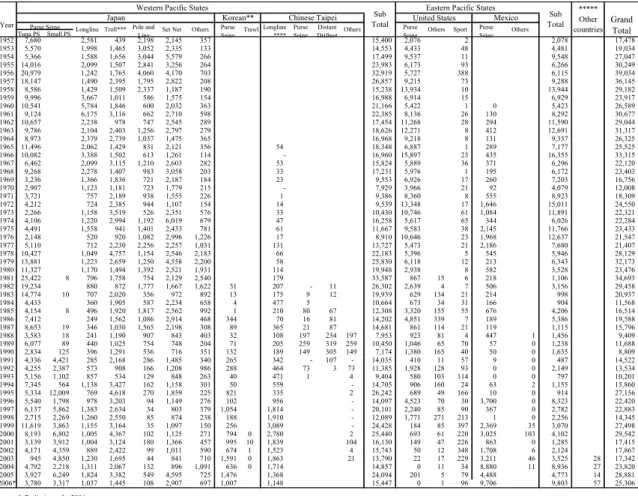
PBF provides important fishery for Japan, Mexico, Taiwan, U.S.A. and South Korea (Anon. 2007). Table 1-1 shows the historical catches by those nations. The PBF catch is mainly from western North Pacific Ocean, which occupies about 84% by Japan, Taiwan and South Korea; from eastern North Pacific by U.S.A. and Mexico. The catches by nations were summarized as followed:
1.1 Japan
Fig. 1-2 shows catch of PBF by Japanese fisheries (Yamada 2007). Japan has used PBF before 1952, including several gears, such as purse seine, longline, troll, pole and line and set net etc. The annual catch varied from 8,000 tons to 30,000 tons. Since 1990s, annual catches ranged from 8,000 tons to 22,000 tons with a 80% age composition about 0-2 years old juveniles, and in particular, 95% in 1991 (Takahashi and Yamada 2002). Yamada and Yamazaki (2002) reported that 70% of Japanese catch (about 5,000 tons to 8,000 tons year to year) were from the coastal purse seine fishery, in which two places were operated, those were the Pacific waters off eastern Japan for juveniles and adults from June to August each year, and off the Sea of Japan for adults from July to August and for juveniles from April to June. Japanese longline was operated at coastal waters off Japan and distant waters in the North Pacific Ocean from late April to early June, including southwestern waters of Miyako Island, southeastern waters of Ishigaki Island and northern waters of Nishimote Island. The annual production varied between 300 and 1,400 tons. Troll fishery was mainly operated in sides of the Sea of Japan from July to March. Catches were almost the juveniles about 20-30 cm. The pole and line fishery fish juvenile PBF incidentally from June to December, with a great variation catches from 100 to 400 tons annually. The Japanese set net fishery exploited size variety PBF in different seasons, the catches were less than 500 tons with main 0 and 1-year-old PBF. And the driffnet fished PBF at coastal waters for juveniles; the catches were less than 100 tons.
of 3,089 tons in 1999, then declined year to year, about 1,400 tons in 2006. 1.3 South Korea
PBF by South Korean fishermen was caught using mackerel purse seiners incidentally from January to August off Cheju and Tsushima. The sizes of caught PBF were about 30-80 cm, equivalent to about o year-old and one-year-old. And the total annual catch was about 1,000 tons with more than 30 purse seiners and 4 trawlers (Anon.2007).
1.4 U.S.A.
The PBF fishery in the eastern Pacific Ocean was exploited from 23oN to 34o30’N, northward to Alaska waters using mainly the purse seiners from May to October. Besides, the recreational fishery was taken by U.S.A. and drift net by Mexico. The annual catches were from 250 tons to 4,900 tons, in which were about 75% were taken from south California and the coastal waters off Mexico (Dreyfus 2007). Also the swordfish and bigeye tuna fisheries can take PBF incidentally by longline gear in the California and Hawaii waters.
1.5 Mexico
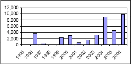
Mexicans took PBF from the coast waters during June and October with a PBF mean weight about 20 kg (5 – 60 kg)。 The catches were from 100 tons to 700 tons annually before 1989 and from 0 to about 9,900 tons then after.
References
Anonymous. 2007. Report of the Fifth Pacific Bluefin Tuna Workshop, Shimizu, Japan. Bayliff, W. H. 1993. Growth and age composition of northern bluefin tuna, Thunnus
thynnus, caught in the eastern Pacific Ocean, as estimated from length-frequency data, with comments on trans-Pacific migrations. Inter-Amer. Trop. Tuna Comm., Bull., 20(9): 501-540.
Bayliff, W. H. 1994. A review of the biology and fisheries for northern bluefin tuna, Thunnus thynnus, in the Pacific Ocean. FAO Fish. Tech. Pap., 336(2) : 244-295. Blackburn, M. 1965. Oceanography and the ecology of tunas. Oceanogr. Mar. Biol.
Ann. Rev., 3: 299-322. Block et al. 1998
Clemens, H. B. 1969. Bluefin tuna migrate across the Pacific Ocean. Calif. Fish and Game, 55(2): 132-135.
Clay, D. (ed.). 1991. Atlantic bluefin tuna (Thunnus thynnus thynnus (L.)): a review. Inter-Amer. Trop. Tuna Comm., Spec. Rep., 7: 89-179.
Collette,B.B. and C.E.Nauen. 1983.FAO species catalogue, Vol. 2. Scombrids of the world; an annotated and illustrated catalogue of tunas, mackerels, bonitos and related species known to date. FAO Fisheries synopsis,125:137 pp.
Cort, J. L. and J. C. Rey. 1985. Analisis de los datos de marcado de atun rojo (Thunnus thynnus L.) en el Atlantico este y Mediterraneo. Migracion, crecimiento y mortalidad. ICCAT, Coll. Vol. Sci. Pap., 22: 213-239.
Deriso, R. B. and W. H. Bayliff (ed.). 1991. World meeting on stock assessment of bluefin tunas: strengths and weaknesses. Inter-Amer. Trop. Tuna Comm., Spec. Rep., 7: 357pp.
Haddon, M. 2001. Modeling and Quantitative Methods in Fisheries. Chapman and Hall/CRC.
Hilborn, R. and C. J. Walters. 1992. Quantitative Fisheries Stock Assessment, Choice, Dynamics and Uncertainty. Chapman and Hall. New York, 570 pp.
Hsu, C. C. 2007. Brief description of revision of north Pacific bluefin tuna catch by Taiwanese fishery. A report submitted to the 2007 Pacific Bluefin Tuna Workshop, Shimizu, Japan. ISC PBF-WG_07_23.
Mather, F. J., III. 1960. Recaptures of tuna, marlin and sailfish tagged in the western north Atlantic. Copeia, 2: 149-151.
Mather, F. J., III. 1980. A preliminary note on migratory tendencies and distributional patterns of Atlantic bluefin tuna based on recently acquired and cumulative tagging results. ICCAT, Coll. Vol. Sci. Pap., 9(2): 478-490.
McAllister, M.K. and Kirkwood, G.P. 1998. Using Bayesian decision analysis to help achieve a precautionary approach for managing developing fisheries. Can. J. Fish. Aquat. Sci. 55: 2642–2661.
Mohn, R.K. 1993. Bootstrap estimates of ADAPT parameters, their projection in risk analysis and their retrospective patterns. In Risk evaluation and biological references points for fisheries management. Ed. by S.J. Smith, J.J. Hunt, and D. Rivard. Canadian Journal of Fisheries and Aquatic Sciences, Special Publication, 120: 173–184.
Nakamura, H. 1938. Preliminary report on the habit of the bluefin, Thunnus orientalis. Zool. Mag. Tokyo, 50: 279-281.
Nakamura, I. and Y. Warashina. 1965. Occurrence of bluefin tuna, Thunnus thynnus (Linnaeus) in the eastern Indian Ocean and the eastern South Pacific Ocean. Nankai Reg. Fish. Res. Lab., Rep., 22: 9-14.
Orange, C. J. and B. D. Fink. 1963. Migration of a tagged bluefin tuna across the Pacific Ocean. Calif. Fish and Game, 49(4): 307-309.
Shingu, C., Y. Warashina and N. Matsuzaki. 1974. Distribution of bluefin tuna exploited by longline fishery in the western Pacific Ocean. Bull. Far Seas Fish. Res. Lab., 10: 109-140.
Smith, S.J., Hunt, J.J., and Rivard, D. 1993. Risk evaluation and biological reference points for fisheries management. Can. J. Fish. Aquat. Sci. Spec Pub, 120. 442 pp. Takahashi, M. and H. Yamada. 2002. Estimation of Pacific bluefin tuna catch at age by
fishery for Japanese fisheries in the north Pacific. ISC BFT-WG/02/DOC13.
Yamada, H. 2007. Reviews of Japanese fisheries and catch statistics on the Pacific bluefin tuna. A paper submitted to the 2007 Pacific Bluefin Tuna Workshop, Shimizu, Japan. ISC PBF-WG_07_01.
Yamada, H. and Y. Yamazaki. 2002. The outline of Japanese offshore purse seine fishery in the Sea of Japan, ISC BET-WG/02
Williams, E.H. and Prager, M.H. 2002. Comparison of equilibrium and nonequilibrium estimators for the generalized production model. Can. J. Fish. Aquat. Sci. 59: 1533–1552.
Table 1-1 shows the historical catches by those nations. (From Report of the 2007 Pacific Bluefin Tuna Workshop, Shimizu, Japan)
Western Pacific States Eastern Pacific States
Year Tuna PS Small PS 1952 7,680 2,581 439 2,198 2,145 357 15,400 2,076 2 2,078 17,478 1953 5,570 1,998 1,465 3,052 2,335 133 14,553 4,433 48 4,481 19,034 1954 5,366 1,588 1,656 3,044 5,579 266 17,499 9,537 11 9,548 27,047 1955 14,016 2,099 1,507 2,841 3,256 264 23,983 6,173 93 6,266 30,249 1956 20,979 1,242 1,765 4,060 4,170 703 32,919 5,727 388 6,115 39,034 1957 18,147 1,490 2,395 1,795 2,822 208 26,857 9,215 73 9,288 36,145 1958 8,586 1,429 1,509 2,337 1,187 190 15,238 13,934 10 13,944 29,182 1959 9,996 3,667 1,011 586 1,575 154 16,988 6,914 15 6,929 23,917 1960 10,541 5,784 1,846 600 2,032 363 21,166 5,422 1 0 5,423 26,589 1961 9,124 6,175 3,116 662 2,710 598 22,385 8,136 26 130 8,292 30,677 1962 10,657 2,238 978 747 2,545 289 17,454 11,268 28 294 11,590 29,044 1963 9,786 2,104 2,403 1,256 2,797 279 18,626 12,271 8 412 12,691 31,317 1964 8,973 2,379 2,739 1,037 1,475 365 16,968 9,218 8 131 9,357 26,325 1965 11,496 2,062 1,429 831 2,121 356 54 18,348 6,887 1 289 7,177 25,525 1966 10,082 3,388 1,502 613 1,261 114 - 16,960 15,897 23 435 16,355 33,315 1967 6,462 2,099 3,115 1,210 2,603 282 53 15,824 5,889 36 371 6,296 22,120 1968 9,268 2,278 1,407 983 3,058 203 33 17,231 5,976 1 195 6,172 23,403 1969 3,236 1,366 1,836 721 2,187 184 23 9,553 6,926 17 260 7,203 16,756 1970 2,907 1,123 1,181 723 1,779 215 - 7,929 3,966 21 92 4,079 12,008 1971 3,721 757 2,189 938 1,555 226 1 9,386 8,360 8 555 8,923 18,309 1972 4,212 724 2,385 944 1,107 154 14 9,539 13,348 17 1,646 15,011 24,550 1973 2,266 1,158 3,519 526 2,351 576 33 10,430 10,746 61 1,084 11,891 22,321 1974 4,106 1,220 2,994 1,192 6,019 679 47 16,258 5,617 65 344 6,026 22,284 1975 4,491 1,558 941 1,401 2,433 781 61 11,667 9,583 38 2,145 11,766 23,433 1976 2,148 520 920 1,082 2,996 1,226 17 8,910 10,646 23 1,968 12,637 21,547 1977 5,110 712 2,230 2,256 2,257 1,031 131 13,727 5,473 21 2,186 7,680 21,407 1978 10,427 1,049 4,757 1,154 2,546 2,183 66 22,183 5,396 5 545 5,946 28,129 1979 13,881 1,223 2,659 1,250 4,558 2,200 58 25,830 6,118 12 213 6,343 32,173 1980 11,327 1,170 1,494 1,392 2,521 1,931 114 19,948 2,938 8 582 3,528 23,476 1981 25,422 8 796 1,758 754 2,129 2,540 179 33,587 867 15 6 218 1,106 34,693 1982 19,234 880 872 1,777 1,667 1,622 31 207 - 11 26,302 2,639 4 7 506 3,156 29,458 1983 14,774 10 707 2,020 356 972 892 13 175 9 12 19,939 629 134 21 214 998 20,937 1984 4,433 360 1,905 587 2,234 658 4 477 5 10,664 673 34 31 166 904 11,568 1985 4,154 8 496 1,920 1,817 2,562 992 1 210 80 67 12,308 3,320 155 55 676 4,206 16,514 1986 7,412 249 1,562 1,086 2,914 468 344 70 16 81 14,202 4,851 339 7 189 5,386 19,588 1987 8,653 19 346 1,030 1,565 2,198 308 89 365 21 87 14,681 861 114 21 119 1,115 15,796 1988 3,583 18 241 1,190 907 843 403 32 108 197 234 197 7,953 923 81 4 447 1 1,456 9,409 1989 6,077 89 440 1,025 754 748 204 71 205 259 319 259 10,450 1,046 65 70 57 0 1,238 11,688 1990 2,834 125 396 1,291 536 716 351 132 189 149 305 149 7,174 1,380 165 40 50 0 1,635 8,809 1991 4,336 4,421 285 2,168 286 1,485 340 265 342 - 107 - 14,035 410 11 57 9 0 487 14,522 1992 4,255 2,387 573 908 166 1,208 986 288 464 73 3 73 11,385 1,928 128 93 0 0 2,149 13,534 1993 5,156 1,102 857 534 129 848 263 40 471 1 4 9,404 580 103 114 0 0 797 10,201 1994 7,345 564 1,138 3,427 162 1,158 301 50 559 - 14,705 906 160 24 63 2 1,155 15,860 1995 5,334 12,009 769 4,618 270 1,859 225 821 335 2 26,242 689 49 166 10 0 914 27,156 1996 5,540 1,798 978 3,203 94 1,149 276 102 956 - 14,097 4,523 70 30 3,700 0 8,323 22,420 1997 6,137 5,862 1,383 2,634 34 803 379 1,054 1,814 - 20,101 2,240 85 90 367 0 2,782 22,883 1998 2,715 2,269 1,260 2,550 85 874 238 188 1,910 - 12,089 1,771 271 213 1 0 2,256 14,345 1999 11,619 3,863 1,155 3,164 35 1,097 150 256 3,089 - 24,428 184 85 397 2,369 35 3,070 27,498 2000 8,193 6,802 1,005 4,367 102 1,125 271 794 0 2,780 2 25,440 693 61 220 3,025 103 4,102 29,542 2001 3,139 3,912 1,004 3,124 180 1,366 457 995 10 1,839 104 16,130 149 47 226 863 0 1,285 17,415 2002 4,171 4,359 889 2,422 99 1,011 590 674 1 1,523 4 15,743 50 12 348 1,708 6 2,124 17,867 2003 945 4,850 1,230 1,695 44 841 710 1,591 0 1,863 21 13,790 22 17 229 3,211 46 3,525 28 17,342 2004 4,792 2,218 1,311 2,067 132 896 1,091 636 0 1,714 14,857 0 11 34 8,880 11 8,936 27 23,820 2005 3,927 6,249 1,824 3,382 549 4,595 725 1,476 1,368 24,094 201 5 79 4,488 4,773 14 28,881 2006* 3,780 3,317 1,037 1,445 108 2,907 697 1,007 1,148 15,447 0 1 96 9,706 9,803 57 25,306 * Preliminary for 2006
** Catch statistics of Korea derived from Japanese Import statistics for 1982-1999, and 2005-2006 as minimum estimates. *** The troll catch for farming estimating 10 - 20 mt since 2000, is excluded.
**** Catches of Chainese Taipei's longline for 2005 and 2006 are preliminary.
***** Other countries include NZ, AUS, Cooks, and so on. Catches derived from Japanese Imort Statistics as minimum estimates.
Others Sport Purse Seine Others Purse Seine Distant Driftnet Sub Total Grand Total Purse
Seine Trawl Longline****
Sub Total ***** Other countries Mexico United States Others Set Net Purse
Seine Others Japan Purse Seine Chinese Taipei Korean**
Longline Troll*** Pole and Line
太平洋黑鮪的分佈
Fig. 1-1 indicates the distribution of PBF in the Pacific Ocean for the species (Collete
and Nauen 1983). (Adapted from Chen Kuo-Shu)
Fig. 1-2 Yearly changes of Pacific bluefin tuna catches by Japanese fleet and by fisheries. (From H. Yamada 2007) 0 5,000 10,000 15,000 20,000 25,000 30,000 35,000 40,000 195 2 195 5 195 8 196 1 196 4 196 7 197 0 197 3 197 6 197 9 198 2 198 5 198 8 199 1 199 4 199 7 200 0 200 3 2006 * Ca tch (m t) Others Handline Drift Net Set Net Pole and Line Troll Longline PS all
0 200 400 600 800 1000 1200 1400 1600 1800 2000 2200 2400 2600 2800 3000 3200 3400 1965 1970 1975 1980 1985 1990 1995 2000 2005 2010 Years C a tc h ( tons ) 1993 Total (small longline mainly)
Drift net
Purse seine others
Fig. 1-3 shows the historical catches of PBF by gears.
2. Abundance index for thelongline fishery targeting spawning Pacific bluefin tuna in the southwestern North Pacific Ocean;
Running title: Abundance index of spawning bluefin tuna
Abundance index for thelongline fishery targeting spawning Pacific bluefin tuna in the southwestern North Pacific Ocean
Hui-Hua Lee * and Chien-Chung Hsu
(Accepted by Fisheries Science and will be published in 74(5), February 2008))
Institute of Oceanography, National Taiwan University, P. O. Box 23-13, Taipei, Taiwan 106. ([email protected]) (Tel: 886-2-23622987; Fax: 886-2-23661198)
* Corresponding author: E-mail: [email protected]
Pacific bluefin tuna Thunnus orientalis Temmincks and Schlegel 1844 is a highly migratory species, distributing over the Pacific Ocean.1 This species is among the quality tunas with high economic values and has been historically exploited mainly by Japanese, USA, Mexican, and Taiwanese fleets. Catches were taken about 10% by Taiwanese fleet after 1999,2 particularly the individuals caught are all giant spawners.3,4 Taiwanese small-scale longliners (vessels less than 100 GRT) target the stock in the southwestern North Pacific from late April through June. Because of significant catch on spawners, any assessment for this stock should include data from Taiwanese fleet.
Many studies and reports were issued to describe the stock status of the Pacific bluefin tuna during the past two decades, however, other than biological studies, the stock assessment was very few with the abundance index derived from Japanese fleets and purse seiners in the eastern Pacific Ocean.2 For this species are exposed to multi-fisheries over most of a wide fishery space extent, historical statistics from different fishing parties should be very essential to indicate its different population patterns. To assess and propose a management measures for the Pacific bluefin tuna, thus, catch and effort data collection as well as developing a reliable abundance index to represent the spawning stock are urged for Taiwanese fishery. Therefore, the objective of the study was to model a time series catch per unit effort (CPUE) that can be used as an index of abundance for the Taiwanese fishery from 1999 to 2004.
Daily catch data from auction records and time records of vessels in-and-out which can trace the fishing effort of each vessel were collected and compiled at Tungkang port in which most of bluefin tuna were landed. A data flow diagram
vessel. Large vessels can store more fish than small ones and may stay at sea longer. Fishing effort was then converted from fishing days to number of hooks operated with assumption of average 1,400 hooks lifted daily. The estimated fishing days were subtracted two days, because the vessel took about one day from Tungkang port to the fishing ground and vice versa.
The catch and effort information were summarized in the form of catch-per-unit-effort (CPUE). Based on the assumption that catch is proportional to the product of fishing effort and density, the ability to use CPUE as an index of abundance depends on being able to remove the influences of factors which change fishing efficiency among vessels and cause differences between trips for the same vessel other than abundance.5 A generalized linear model (GLM)6 was applied to remove the influential factors and, in the present analysis, the available factors for each vessel-trip compiled in the catch and effort data include year (1999-2004); month (May and June); size of vessel (3 levels, 10-20 GRT, 20-50 GRT and 50-100 GRT). Considering all bluefin fisheries from western North Pacific, Taiwanese fishery appears to be a local fishery with marked fishing season even though the detailed fishing positions are not available and therefore, spawning bluefin density was assumed to be spatially homogeneous.
Independent variables considered for GLM are fishing year, month, size of vessel, and two-way interaction among month and size of vessel, and the dependent variable is the logarithm of catch per unit effort (lnCPUE) assuming a Gaussian error distribution. To avoid zero CPUE causing failure taking with the logarithmic transformation, a positive constant value was added to all CPUEs, while maintaining or achieving
residuals before choosing the value. The assumption of a GLM is that the relationship between the expected lnCPUE and the independent variables is linear. The full model is,
ijk k j k j i ijk c Y M S M S CPUE + )=μ+ + + + × +ε ln( (1)
where μ is overall mean, c is a constant that is decided in test runs, Y is the effect i of year i, Mj is the effect of month j, S is the effect of size of vessel k, k Mj×Sk is
the two-way interaction term between month j and size of vessel k , and ε is error ijk term with N
(
0,σ . Due to the difficulty of explaining interaction between year factor 2)
and other factors, only interaction between month and size of vessel was considered. A step-wise analysis of deviance was performed to determine the set of systematic factors and interactions that significantly explained most of the observed CPUE variability. The Chi-square (χ2) statistic was used to test the significance of an
additional factor in the model.8 Final selection of explanatory factors was conditional on significance of the χ2 test and percent change in deviance as each factor is added to the
model. The ln CPUE c
(
+ was estimated as the least squares means (LS means) of the)
factors selected and then back transformed to derive the standardized CPUE. The analyses were run with the SAS GENMOD and GLM procedures (SAS Inst. Inc.).Figure 2 illustrates the normality of residuals from the transformed data by adding different constant values. The normality was visually diagnosed by comparing quantile of residuals with the 45 degree reference line on the Q-Q plot, indicating that the Q-Q plot derived by adding 1 or 0.01 as a constant departed from the line more than that by adding 0.1 or 10% of overall mean. More specifically, the Q-Q plot for the data with
5). These data suggest that both 0.1 and 10% of overall mean as a constant capture the normality of residuals, but the value of 0.1 shows better fit of data at the right side than 10% of overall mean.
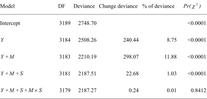
Results of deviance estimated from step-wise regression are presented in Table 1 indicating that factors of year, month, and the size of the vessel were significant for χ2
test (Pr(χ2)<0.0001). Among these factors, year or month explained over 5% of
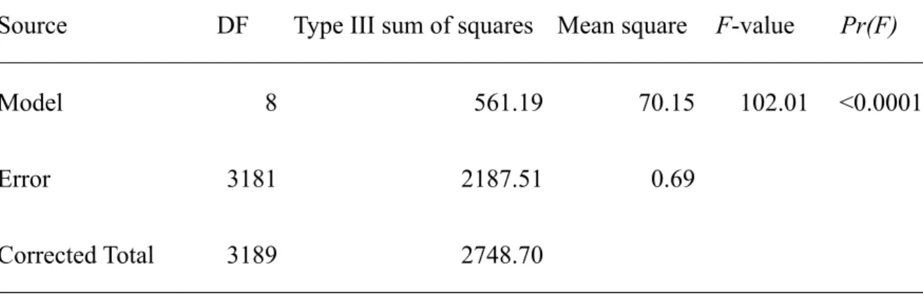
deviance, whereas size of vessel explained 1% of deviance. Therefore, factors of year, month, and size of vessel were selected into GLM. The result of ANOVA is shown in Table 2.
Estimated CPUE by GLM is illustrated in Figure 3. Annual abundance index sharply declined from 0.46 fish per 1,000 hooks in 1999 to 0.14 fish per 1,000 hooks in 2002, and remained constant at 0.2 fish per 1,000 hooks in 2003 and 2004.
The process attempts to remove most of the annual variation in the data that do not attribute to changes in abundance and the annual index reflects population abundance. In this study, the selected factors explained about 20% of variance of the data (Table 1) and explanatory power of the model (R2) were 0.2 (Table 2). Maunder and Punt9
indicated that the explanatory power is not always satisfactory and it can be increased by involving in more explanatory variables. Accordingly, the explained variation is not the absolute quantity to judge the reliability of index of abundance. Instead, it is more important to consider whether the time series of abundance index accurately reflects changes in catchability and fisheries. First, declined catches from the longline fisheries2 consists with our result shown in Fig. 3, which is low abundance of bluefin tuna in 2002. Second, abundance indices of spawning fish caught by Japanese costal longliners also
standardized CPUE in this study is a useful abundance index for spawning bluefin tuna targeted by Taiwanese small-scale longline fishery.
The rapid development of the Taiwanese small-scale longline fishery targeting spawning stock brought about high fishing pressure on the large bluefin in recent ten years. Taking into account the size specific seasonality of fishery target spawning bluefin tuna by Taiwanese longliners, the index of abundance estimated in the present study could provide important information to advance future stock assessment.
ACKNOWLEDGEMENTS
This study is a result of work sponsored by the National Science Council under grant NSC93-2313-B-002-015 ¸NSC93-2313-B-002-041 and NSC93-2313-B-002-055 to C. C. Hsu.
References
1. Bayliff WH. A review of the biology and fisheries for northern bluefin tuna, Thunnus
thynnus, in the Pacific Ocean. FAO Fish. Tech. Pap.1994; 336: 244–295.
2. Anonymous. Report of the Fourth ISC Meeting of the Pacific Bluefin Tuna Working Group. Interim Scientific Committee for Tuna and Tuna-Like Species in the North Pacific Ocean. ISC/06/Plenary/7, ISC, 2006.
3. Hsu CC, Liu HC, Wu CL, Huang ST, Liao HK. New information on age composition and length-weight relationship of bluefin tuna, Thunnus thynnus, in the southwestern
985-994.
5. Gulland JA. Fish Stock Assessment: A Manual of Basic Methods. Wiley, New York. 1983.
6. Nelder JA, Wedderburn RWM. Generalized linear models. J. R. Stat. Soc. Se. A. 1972; 137: 370–384.
7. Berry DA. Logarithmic transformations in ANOVA. Biometrics. 1987; 43: 439-456. 8. McCullagh P, Nelder JA. Generalized Linear Models. 2nd edn. Chapman and Hall,
London. 1989.
9. Maunder MN, Punt AE. Standardizing catch and effort data: a review of recent approaches. Fish. Res. 2004; 70: 141-159.
Figure captions
Fig. 1 Data flow diagram of Taiwanese longline fishery targeting Pacific bluefin tuna showing data sources (the top of the diagram), processing (in the middle of the diagram) and flowing into the catch and effort database, where arrows indicate the direction of data flow. T1 and T2 represent date of auction and
disembarkation time, respectively and the time difference (T1 -T2≤3) is in need
of quality of fish meat.
Fig. 2 The Q-Q plots of residuals of transformed data by adding different constant values (0.01, 0.1, 1, and 10% of overall mean) to the observations from GLM against the corresponding quantiles of a standard normal distribution, where mu and sigma represent mean and standard deviance of residuals of transformed data, respectively.
Fig. 3 Estimated and observed CPUE of Pacific bluefin tuna targeted by Taiwanese longline fishery. The lines represent 1 standard error.
Fig. 1
1. Merging: catch with matching effort; 2. Time difference: (T1-T2) 3 days;
3. Targeting: May and June.
Catch&effort Catch database Source: Fishermen’s Association Variables: date of auction, name of vessel, number of fish Effort database Source: Security Inspect Station Variables: name of vessel, size of vessel, embarkation time, disembarkation time ≤
Fig. 2 -2 0 2 -3 -2 -1 0 1 2 3 -2 0 2 -0 .5 0 .0 0 .5 1 .0 1 .5 -2 0 2 -4 -2 0 2 4 Normal Quantiles -2 0 2 -2 -1 0 1 2 3 Constant= 0.01 Normal parameters Mu 0 Sigma 1.433959 Normal parameters Mu 0 Sigma 0.828223 Normal parameters Mu 0 Sigma 1.003785 Normal parameters Mu 0 Sigma 0.304053 Resid ual s Constant= 0.1 Constant= 1 Constant= 10% of overall mean -2 0 2 -3 -2 -1 0 1 2 3 -2 0 2 -0 .5 0 .0 0 .5 1 .0 1 .5 -2 0 2 -4 -2 0 2 4 Normal Quantiles -2 0 2 -2 -1 0 1 2 3 Constant= 0.01 Normal parameters Mu 0 Sigma 1.433959 Normal parameters Mu 0 Sigma 1.433959 Normal parameters Mu 0 Sigma 0.828223 Normal parameters Mu 0 Sigma 0.828223 Normal parameters Mu 0 Sigma 1.003785 Normal parameters Mu 0 Sigma 1.003785 Normal parameters Mu 0 Sigma 0.304053 Normal parameters Mu 0 Sigma 0.304053 Resid ual s Constant= 0.1 Constant= 1 Constant= 10% of overall mean
Fig. 3 CP UE (number of fish / 1,000 hooks) 0.0 0.1 0.2 0.3 0.4 0.5 0.6 0.7 0.8 0.9 1.0 1999 2000 2001 2002 2003 2004 0 . 0 0 . 1 0 . 2 0 . 3 0 . 4 0 . 5 0 . 6 0 . 7 0 . 8 0 . 9 1 . 0 1 9 9 92 0 0 02 0 0 12 0 0 22 0 0 32 0 0 4Estimated CPUE Observed CPUE CP UE (number of fish / 1,000 hooks) 0.0 0.1 0.2 0.3 0.4 0.5 0.6 0.7 0.8 0.9 1.0 1999 2000 2001 2002 2003 2004 0 . 0 0 . 1 0 . 2 0 . 3 0 . 4 0 . 5 0 . 6 0 . 7 0 . 8 0 . 9 1 . 0 1 9 9 92 0 0 02 0 0 12 0 0 22 0 0 32 0 0 4Estimated CPUE Observed CPUE CP UE (number of fish / 1,000 hooks) 0.0 0.1 0.2 0.3 0.4 0.5 0.6 0.7 0.8 0.9 1.0 1999 2000 2001 2002 2003 2004 0 . 0 0 . 1 0 . 2 0 . 3 0 . 4 0 . 5 0 . 6 0 . 7 0 . 8 0 . 9 1 . 0 1 9 9 92 0 0 02 0 0 12 0 0 22 0 0 32 0 0 4Estimated CPUE Observed CPUE
Table 1 Analysis of deviance table of explanatory variables in GLM. Percentages of deviance refer to the percentages of change in deviance divided by deviance in
previous model, and Pr(χ2) values indicate the 5% Chi-square probability between
consecutive models.
Model DF Deviance Change deviance % of deviance Pr(χ2)
Intercept 3189 2748.70 <0.0001
Y 3184 2508.26 240.44 8.75 <0.0001
Y+M 3183 2210.19 298.07 11.88 <0.0001
Y+M + S 3181 2187.51 22.68 1.03 <0.0001
Table 2 Analysis of variance (ANOVA) table for the selection model in GLM.
Source DF Type III sum of squares Mean square F-value Pr(F)
Model 8 561.19 70.15 102.01 <0.0001
Error 3181 2187.51 0.69
Corrected Total 3189 2748.70
3. Incorporating uncertainty into the estimation of biomass for the Pacific bluefin tuna
Running title: production analysis by Bayesian approach for Pacific bluefin tuna
Hui-Hua Lee 1 and Chien-Chung Hsu1,*
1Institute of Oceanography, National Taiwan University, P. O. Box 23-13, Taipei,
Taiwan 106. (Tel: 886-2-23622987; Fax: 886-2-23661198)
* Corresponding author: E-mail: [email protected]
Key Words: Pacific bluefin tuna; Bayesian approach; production analysis; uncertainty; maximum sustainable yield
Introduction
Pacific bluefin tuna Thunnus orientalis Temmincks and Schlegel 1844 is a highly migratory species, distributing over the Pacific Ocean (Bayliff, 1994). This species is among the quality tunas with high economic values and has been historically exploited mainly by Japanese, USA, Mexican, and Taiwanese fleets. Since 2000, Japanese fleets, which targeted all the fish sizes around the year, have taken about 66%..USA fleets, which caught almost juveniles, have taken about 2%. Mexican purse seiners for juveniles have taken about 20%. Taiwanese fleets, which targeted all giant spawners (Hsu et al., 2000; Chen et al., 2006), have taken bout 10%. Recently, the state of this stock was evaluated by Food and Agriculture Organization of the United Nations and the stock was listed in fully exploitation (Maguire et al., 2006). However, this doesn’t provide estimates of stock status such as relative biomass and its exploitation rate and reference points.
Biomass dynamic models are one of the simplest analytical methods available that focuses on the dynamics of the population as a whole. The original method of assuming equilibrium conditions has been criticized for providing overly optimistic estimates of optimum effort and maximum sustainable yield and suggestions were made to abandon the use of the models (Hilborn and Walters, 1992; Haddon, 2001; Williams and Prager, 2002). The major concerns about fitting these models to time-series data are that uncertainties and variability are not taken into consideration. Parameters are point estimates or assumed values are used and uncertainties of parameters are often ignored or additional analyses are conducted to assess uncertainties using sensitivity analysis (e.g. Goodyear, 1995), confidence intervals (e.g. Mohn, 1993) or sampling distributions using re-sampling methods (e.g. Smith et al., 1993). However, none of these provide integrated analyses to describe unknowns and parameters in the form of probability for complex model (McAllister and Kirkwood, 1998). Further uncertainties are associated with how the model handles observation and process errors. If only observation error explains randomness, then the population dynamics will be deterministic, population abundance could not be accurately estimated. If there is only process randomness, then population size would be estimated perfectly, but ignores the random errors in the observations. In reality, both types of error almost certainly occur.
interest such as maximum sustainable yield.
Materials and methods
Data usedThe building blocks for assessing Pacific bluefin tuna are observations on stock size and removal and hypothesis (model) of how they relate in time space. Reliable catch data and indices of abundance are two key inputs for population dynamic models. We obtained Pacific bluefin tuna harvest data from the International Scientific Committee on Tuna and Tuna-like Species in the North Pacific Ocean (ISC) between 1952 and 2006. Abundance indices were available for six major fisheries, Japanese offshore longliners (1952-2005), Japanese coastal longliners (1994-2005), Taiwanese coastal longliners (1999-2005), eastern Pacific Ocean purse seiners (1960-2004), Japanese purse seiners (1981-2004), and Japanese troll fisheries (1981-2004).
Surplus production models
Biomass dynamic models are one of the simplest analytical methods available that provide for a full fish stock assessment when the measurements on the fishery consist of the annual catches and measures of abundance indices for a number of years are available. The current biomass is related to previous biomass plus term for surplus production in previous time minus term for catch. The (deterministic) state equation for the total biomass is
(1) where B is the biomass of the stock that is vulnerable to fishing at the start of year t, t
t
C is the catch during year t, and the surplus production function g(B) quantifies
the overall change in biomass due to growth, recruitment and natural mortality (Ricker, 1975). The surplus production function is assumed to be nonnegative with
0 ) ( ) 0 ( =g K =
g , where K is the carrying capacity resulting from the effect of finite resources in combination with environmental variability, food and space limitations. The quadratic Schaefer (1954) form of surplus production function is
⎟ ⎠ ⎞ ⎜ ⎝ ⎛ − = − − − K B rB B g t t t 1) 1 1 1 ( (2) 1 1 1 ( ) ˆ − − − + − = t t t t B g B C B
maximum reproductive rate). This function takes its maximum values of rK when 4 biomass is half of K. This maximum value is often regarded by management as the maximum surplus production (MSP).
Surplus production functions are fitted to annual indices of abundance. The index for each fishery is assumed to vary proportionally to stock biomass with constant catchability for that fishery. By assuming that abundance indices are correlated measures of population abundance, the model is able to incorporate multiple indices by interpreting differences among indices as sampling error. The (deterministic) observation equation is t i i t q B I , = (3)
where It,i is biomass indices for fishery i and q is the catchability coefficient for i
fishery i.
General framework for Bayesian stock assessment
The Bayesian approach to stock assessment in general consists of two steps: (i) constructing a full probability model that consists of a joint probability distribution for all observable (here the CPUEs) and unobservable quantities (here the biomasses and model parameters) and (ii) calculating the posterior distribution by conditioning on the observed data, i.e. the conditional probability distribution of the unobservable quantities of interest, given the observed data.
In the first step, the joint probability density p(Y,Θ) of the observations )
,..., (y1 yN
Y = and the unobservable quantities, state spaces,Θ=(θ1,...θn) can be written as the product of two densities, referred to as the prior density p(Θ) and the sampling density or likelihood function p(YΘ):
) ( ) ( ) , (Y Θ = p Θ p YΘ p (4)
In the second step, parameter estimation is a procedure of updating the prior distributionp(Θ), which describes the uncertainty about the parameter values prior to
∫
Θ Θ Θ Θ Θ Θ = Θ Θ = Θ d Y p p Y p p Y p Y p p Y p ) ( ) ( ) ( ) ( ) ( ) ( ) ( ) ( ∝ p(Θ)p(YΘ) (5), where p(Y) is a normalization constant, which involved in formidable high-dimensional integration for state-spaces Θ . Bayesian inference entails the evaluation of various summaries of a specific component θi, such as moments and quantiles. This requires integration, with respect to θi, of the joint posterior p( YΘ ). These integrals are evaluated via Markov chain Monte Carlo (MCMC) methods (Gilks et al. 1996), which Monte Carlo simulation from a Markov chain that is constructed whose stationary distribution is the joint posterior distribution. After running sufficiently long Markov chain to find the region of the state space with the highest density and burning-in pre-convergence values, one obtains (correlated) samples from the posterior distribution. Then the histogram of samples is used as an approximation.
The Gibbs sampling (Geman and Geman, 1984) is a specific MCMC method for sampling from the joint posterior distribution,p(θ1,θ2,...,θnY), where Θ=(θ1,...θn) are the unknowns and Y denotes the observables. Given an arbitrary set of starting vector Θ(0)=( (0) (0)
1 ,...,θn
θ ), the algorithm proceeds by sampling from the each of the full conditional posteriors as follows:
Simulate ~(1) 1 θ ( (0),..., (0), ) 2 1 Y pθ θ θn Simulate ~(1) 2 θ ( , (0),..., (0), ) 3 ) 1 ( 1 2 Y pθ θ θ θn M Simulate (1) ~ n θ ( ,..., (1), ) 1 ) 1 ( 1 Y pθnθ θn−
We obtain an updated vector ( 1,..., 1) 1 1
n
θ θ
θ = and start the procedures again by using previous vector to get θ . Repeat m iterations until convergence, this yields 2
) ,..., ( ( ) ( ) 1 ) ( m n m m θ θ
State-space modeling of biomass dynamics using a Bayesian approach
A Bayesian state-space formulation of the Schaefer surplus production model was developed by Millar and Meyer (2000) and an extension of their model forms the basis for biomass dynamics analyses of Pacific bluefin tuna. The model includes observation errors in indices of abundance and process errors between model-derived biomass and the true biomass. The model also takes into account uncertainties in catch data and estimates biomass from the six primary fisheries. There are 54 years of indices of abundance data and catch biomass (1952-2005). In the model, the years are sequentially named from year1 for 1952 to year 54 for 2005.
Modeling
The Bayesian surplus production (BSP) model uses a re-parameterized form of the Schaefer surplus production model (equ. 2). Re-parameterization was carried out to increase the Markov chain mixing speed and to reduce parameter correlations (Gill, 2002). The re-parameterized form relates the fraction of carrying capacity (Pt =Bt K) to intrinsic growth rate, carrying capacity, and the catch time series. The expected Pˆ is calculated as:t
Pˆ1 =1 for t=1 K C P rP P P t t t t t 1 1(1 1) 1 ˆ − − − − + − − = for t≥2 (6)
Index for each fishery is assumed to be proportional to stock biomass with constant catchability for each fishery, i, proportionality assumption. The expected Iˆ for t,i each fishery is calculated as:
i t
Iˆ, =qiKPt (7) where q is the catchability coefficient for each fishery. These relationships are the i basis of the state equations for the state-space model, which errors exist between
i t i t i t I v I ,) log(ˆ,) , log( = + (8)
where μtand vt,i are independent and identically normal distributed N(0,σ2) and )
, 0
( 2
i
N τ random variables, respectively. Abundance indices were weighted equally
within the model.
Uncertainties about true catches
Errors of catch biomass are likely made from various sources of catch estimation and raised catch values etc. Reported catch biomass were likely measured with error but were unbiased. Therefore to incorporate this uncertainty, we modeled the true catch for entire time series using a uniform distribution with a 10% coefficient of variation to describe variability of reported catch.
)] ˆ ( ), ˆ [( ~ ˆ ˆ t t t C C t t uniform C C C −σ +σ (9)
where C and t Cˆ are the true and reported catches in year t and t
t
Cˆ
σ (=10%Cˆ ) is t the standard deviation for the true catch in year t.
The likelihood
Due to vt,iis assumed to be normal distributions with parameters 2 i
τ , the It,i
then follow lognormal distributions by the equation 8. Given Iˆ , the likelihood for t,i It,i is
) ( 2 ,i i t I L τ = i τ π 2 1
(
)
⎟ ⎟ ⎠ ⎞ ⎜ ⎜ ⎝ ⎛ − − 2 2 , , 2 ) ˆ log( ) log( exp i i t i t I I τ (10)Specifying prior distribution
and 54 ratios of biomass to the carrying capacity (P :t 1≤ t≤54). The joint prior density p(K, r,σ ,2
i
q , 2
i
τ ,P ) is obtained from the prior t p(K, r,
2
σ ,q ,i 2 i
τ ) and the distribution of (Pt K,r,σ2 ) determined from the state equation
(equ. 6), ( p K, r,σ ,2 i q , 2 i τ ,P ) =t p(K, r,σ ,2 i q , 2 i τ )p( Pt K,r,σ2 ) =p(K, r,σ ,2 i q , 2 i τ ) p( P1 σ )2
∏
= − 54 2 2 1, , , ) ( t t t r K P P p σ (11) which ( , , , 2) 1 K r σ P Pp t t− terms are implicitly conditioning on the catches C . t
For simplicity, it will be assumed that each if the parameters is mutually independent in the joint prior density of (K, r,σ ,2
i
q , 2
i
τ ). Therefore, priors for each of the parameters can be constructed independently
( p K, r,σ ,2 i q , 2 i τ )= p(K) p(r) p(σ2) ( ) i q p ( 2) i p τ (12) where p(K),p(r),p(σ2), ( ) i q p , and ( 2) i
p τ are the prior for the parameter value K,
r,σ ,2 i q , and 2 i τ . K — carrying capacity
A prior distribution for K that is fully no informative because there is no previous work on production model for Pacific bluefin tuna and carrying capacity is stock-specific, which means that values for other related species might not be incorporated.
Thus, the prior for K can be regarded as scale parameters and a no informative prior is therefore uniform on log scale, K~uniform[log(33),log(500)] (in thousands of tons). The lowest bound is approximately equal to the largest observed catch in the
r — intrinsic growth rate of population
A prior for r that is non-informative would be restricted to r~uniform[0.01, 1], where the lower and upper bounds are considered to be very small and large values for r for tuna, respectively.
2
σ and 2 i
τ — process error variance and observation error variance
Conjugate priors can be constructed for the process error variance σ and the 2
observation error variance 2 i
τ in the normal models and therefore, their posterior distributions follow the same parametric form as the priors (Appendix A). An inverse gamma distribution with parameters α(>0) andβ (>0) was specified for the prior of both σ and 2 2
i
τ . The inverse gamma specification is articulated from the gamma statements through convention of specifying precisions instead of variances in normal specification. Carlin and Louis (2001) suggest solving the moment equations for α andβ using empirical mean and standard deviation as follows.
The first and second moments for the inverse gamma distribution are: μ = 1 − α β , for α>1 2 s = ) 2 ( ) 1 ( 2 2 − − α α β , for α>2 Then, α= 2 2 2 + s μ β = ⎟⎟ ⎠ ⎞ ⎜⎜ ⎝ ⎛ +1 2 2 s μ μ
A vague inverse gamma prior with high standard deviation was chosen and mean was set to be equal to its standard deviation so as to the fraction μ2 s2 is unity.
Thus, a vague inverse gamma distribution with mean and standard deviation equal to 50 was chosen so that α is 3 and β is 100. The inverse gamma specification is articulated from the gamma statements through convention of specifying precisions
i
q — catchability for each fishery
There was no information available that could be used to develop an informative prior for catchability coefficient for each fishery. Therefore, a uniform prior was chosen for q on log scale, i q ~i uniform[log(10−5),log(102)]. The quantity log( )
i
q can be regarded as an intercept term in the observation-error model (Kass and Wasserman, 1996).
Sampling from the posterior distribution
In order to construct a posterior probability density function of model input parameter, the steps referred to the Bayesian estimation are described as follows. In the first step, the joint posterior probability density was the product of the prior density and likelihood of the data.
( p K, r,σ ,2 i q , 2 i τ ,Pt It,i)∝ (p K, r,σ ,2 i q , 2 i τ ,P )t
∏
= 54 1 2 , , , ) ( t i i t i t P q I L τ =p(K, r,σ ,2 i q , 2 i τ )p( P1 σ )2∏
= − 54 2 2 1, , , ) ( t t t r K P P p σ∏
= 54 1 2 , , , ) ( t ti t i i q P I L τ (13)In the second step, the Gibbs sampler was used to sample from the joint posterior density (equ. 13). This requires each of the univariate full conditional posterior densities for all 69 unobservable in the model to be sampled in turn. The full condition posterior density of a certain parameter θi can be constructed from the joint posterior of Θ by extracting the terms that involve θi (Appendix B). The other terms in the posterior simply are regarded as the normalizing constant.
We performed 100, 000 cycles of the Gibbs sampler and the results of the first 5,000 cycles were discarded as a burn-in period. For the remaining 95,000 cycles, every 10th observation was thinned (saved) to avoid highly correlated values, which yielded a final chain of length 9,500. Convergence of the simulations was tested using the Geweke test (1992), the Heidelberger and Welch test (1983), the Rftery and Lewis (1992) from the package BOA (“Bayesian Output Analysis”) (Smith 2005) of R software (R Development Core Team 2004).
The Raftery and Lewis convergence diagnostics confirmed that the thinning of the chain, burn-in period, and the number of iterations were sufficient. Lags and autocorrelations within each parameter chain were reasonably low. Geweke’s Z scores do not fall within the extreme tails of a standard normal distribution, suggesting that the chain fully converged. Trace plots and running mean from the end of the burn-in period are shown in Fig. 1. All parameters and the states appear to be stable in the trace plots of path of the Gibbs sampler runs and have settled into a stable running mean. All together, the tests and graphical diagnostics showed no evidence against convergence.
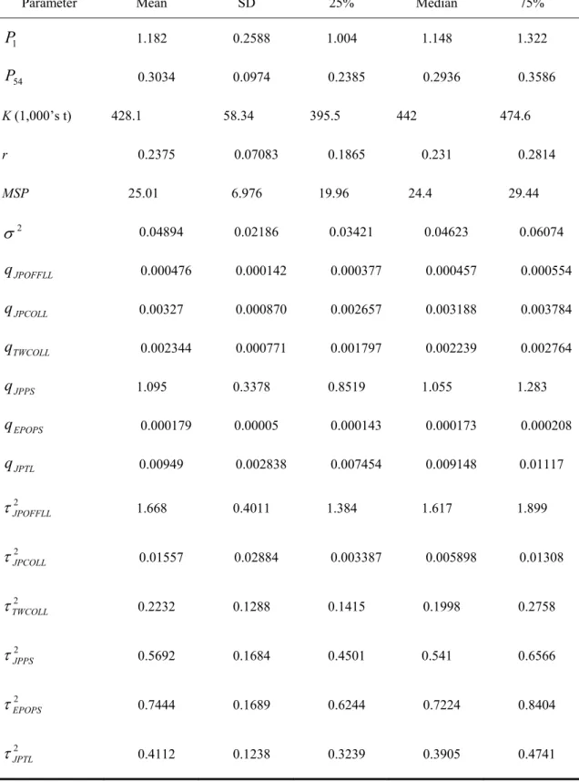
Kernel estimates for the marginal posterior densities for the above unknowns are demonstrated in Fig. 2. Summary statistics including mean, standard deviation, and 25, 50, and 75% quantiles are given in Table 1. As can be seen from the kernel density plots in Fig. 2, the posterior distributions show single mode and become sharper than priors distributions for K, r, and q with the uniform priors and i σ and2 2
i
τ with the vague inverse gamma priors.
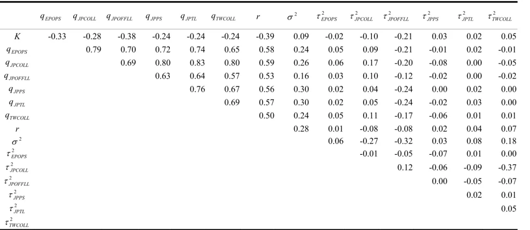
There are considerable correlations between parameters of K, r, q andi σ , 2
whereas the correlations between the other parameters are low (Table 2). Correlations among q are higher than those between parameters of K, r, i q andi σ whereas 2
correlations among 2 i
τ are low. This implies that abundance indices are correlated measures of population abundance and the difference among them is mainly from sampling error.
The posterior distributions showed that most of the observation error variances (τ ) are substantially larger than the process error variance (2 σ ) except for the 2
Japanese coastal longliners (Table 1, Fig. 2). The higher posterior densities on the observation error variances correspond to more variability in the data than in the dynamics model.
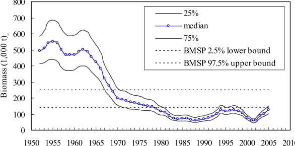
The posterior distribution of the maximum surplus production MSP has a mean of 25.01 ± 6.976 (thousand tons). The biomass that could produce maximum surplus production was estimated as 214.05 (thousand tons) which is the half of the estimated mean of K (Table 1). The posterior medians and uncertainties of the biomasses were
to increase in recent years. As for the forecast, the surplus production model predicts a biomass with posterior mean equal to 116.8 ± 57.22 for the following year 2006.
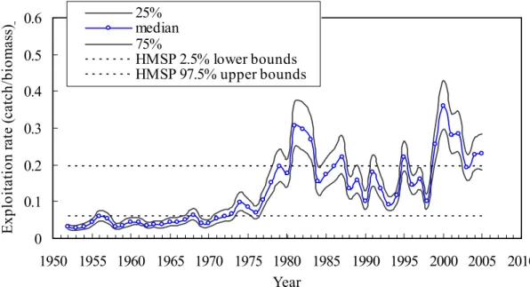
The posterior medians and uncertainties of the exploitation rate (catch/biomass) were shown in Fig. 4. The exploitation rates prior to 1970 are relatively low, whereas those after 1970 fluctuate over 2.5% quantile of exploitation rate at maximum surplus production. The situation is severe in the beginning of 1980s and in recent years probably due to the commencement of the surface fisheries and the longliners (Fig. 5).
A comparison between the observed CPUEs and the posterior predictive distribution of the CPUEs was made by overlaying the 95% posterior predictive intervals for CPUEs onto a plot of the observed CPUEs (Fig. 5). Predicted CPUEs do not follow strictly the observed CPUEs. In particular, poorly prediction were found in the early years for the Japanese offshore longliners resulting in large observation error variance with high standard deviation (Table 1 and Fig. 2). It might imply that catchability is not constant over the time period for the Japanese offshore longliners. Outliners are detected for others fisheries but most of the 95% predicted CPUEs overlaid by the observed CPUEs.
Discussion
This paper has presented a fully specified stochastic population dynamics for Pacific bluefin tuna containing both deterministic equations and the assumption about randomness. This is accomplished using a Bayesian approach to statistical inference via the Gibbs sampler and unrealistic assumptions made by the original population were overcome. The harvest was not assumed to equal surplus production (Quinn and Deriso, 1999) and the parameters were not assumed to be constant. This allows us to build hierarchical models with random-effect, handle arbitrary distributional assumptions for priors, and simultaneously estimate process and observation error. Further extension on stochastic historical catches was also considered because the catch figures usually provide the mean of catches.
A Bayesian stock assessment requires prior knowledge of various parameters to be incorporated into the analysis and careful consideration of the choice of prior (Punt and Hilborn, 1997; 2001). In the surplus production model, all parameters are defined on the positive real number and thus the lognormal, gamma and uniform distributions that include the positive are appropriate. Informative prior can be referred to similar
parameters (uniform on log scale). Gelman et al. (1995) recommended using vaguely informative priors to allow the data to have more weight in shaping the posterior distribution. Accordingly, we formulated vague inverse gamma distributions for the process and observation error variances. The posterior distributions for these key parameters showed sharper distributions than uniform and vague inverse gamma prior distributions (Fig. 2). This implies that the prior loses its influence on the shape of the posterior and data are informative. The choice of priors seems to be reasonable in the present study.
The Bayesian state–space model improves on the two estimators, the observation error estimator and process error estimator. The observation error estimator includes the observation error but ignores the process error, whereas the process error estimator includes the process error but disregards the observation error. In the Bayesian analysis, measurement and process errors are clearly separated and the precision of error variance estimates can be assessed in detail from the posterior densities (Fig. 2). Hilborn and Walters (1992) and Polacheck et al. (1993) found that the process error estimator produces less reliable estimates than the observation error estimator, which is generally regarded to be the best approach when only one error structure is considered. Our study indicates that the observation error variances excluding the Japanese coastal longliners are larger than the process error for modeling Pacific bluefin tuna population using the biomass dynamic model (Table 1). The prediction of CPUEs for Japanese coastal longliners was superior to those for others fisheries, resulting in a small observation error variance. These findings may suggest that when more than one index was used in the models, the observation errors should be incorporated into modeling to produce reliable parameter estimates.
Reference
Anonymous. Report of the Fourth ISC Meeting of the Pacific Bluefin Tuna Working Group. Interim Scientific Committee for Tuna and Tuna-Like Species in the North Pacific Ocean. ISC/06/Plenary/7, ISC, 2006.
Bayliff WH. A review of the biology and fisheries for northern bluefin tuna, Thunnus
thynnus, in the Pacific Ocean. FAO Fish. Tech. Pap.1994; 336: 244–295.
Carlin, B.P. and Louis, T.A. 2001. Bayes and empirical Bayes methods for data analysis. Second edition. Chapman & Hall/CRC, New York.
Carlin, B.P., Polson, N.G., and Stoffer, D.S. 1992. A Monte Carlo approach to nonnormal and nonlinear state-space modeling. J. Am. Statist. Ass. 87: 493-500. Casella, G. and Berger, R.L. 2002. Statistical inference. Second edition. Duxbury
Advanced Series.
Chen, K.S., Crone, P., and Hsu, C.C. 2006. Reproductive biology of female Pacific bluefin tuna Thunnus orientalis from south-western North Pacific Ocean. Fish. Sci. 72: 985-994.
Gelman, A., Carlin, J.B., Stern, H.S., and Rubin D.B. 1995. Bayesian data analysis. Chapman&Hall.
Geman, S. and Geman, D. 1984. Stochastic relaxation, Gibbs distributions and the Bayesian restoration of images. IEEE Transactions on Pattern Analysis and Machine Intelligence. 6: 721-741.
Gilks, W.R., Richardson, S., and Spiegelhalter, D.J. 1996. Markov Chain Monte Carlo in Practice. Chapman and Hall, London, UK.
Gill, J. 2002. Bayesian methods: A social and behavioral sciences approach. Chapman & Hall/CRC.
Geweke, J. 1992. Evaluation of the accuracy of sampling-based approaches to calculating posterior moments. In Bayesian statistics 4. Edited by J.M. Bernardo, J.O. Berger, A.P. Dawid, and A.F.M. Smith. Oxford University Press, Oxford, U.K. pp. 169-193.
Goodyear, C.P. 1995. Red snapper in US waters of the Gulf of Mexico. MIA-95/96-05. Southeast Fisheries Science Center. Miami, FL.
Haddon, M. 2001. Modeling and Quantitative Methods in Fisheries. Chapman and Hall/CRC.
Heidelberger, P. and Welch, P. 1983. Simulation run length control in the presence of an initial transient. Oper. Res. 31: 1109-1144.
Kass, R.E. and Wasserman, L. 1996. The selection of prior distributions by formal rules. J. Am. Statist. Ass. 91: 1343-1370.
Ludwig, D. and Walters, C.J. 1981. Measurement errors and uncertainty in parameter estimates for stock and recruitment. Can. J. Fish. Aquat. Sci. 38: 711–720.
Ludwig, D., Walters, C.J., and Cooke, J. 1988. Comparison of two models and two estimation methods for catch and effort data. Nat. Res. Model. 2: 457–498.
Maguire, J.J., Sissenwine, M., Csirke, J., Grainger, R., and Garcia, S. 2006. The state of world highly migratory, straddling and other high seas fishery resources and associated species. FAO Fisheries Technical Paper. No. 495, Rome, FAO. 84 pp. McAllister, M.K. and Kirkwood, G.P. 1998. Using Bayesian decision analysis to help
achieve a precautionary approach for managing developing fisheries. Can. J. Fish. Aquat. Sci. 55: 2642–2661.
Millar, R.B., and Meyer, R. 2000. Non-linear state space modelling of fisheries biomass dynamics using Metropolis-Hastings within-Gibbs sampling. Appl. Stat. 49, 327–342.
Mohn, R.K. 1993. Bootstrap estimates of ADAPT parameters, their projection in risk analysis and their retrospective patterns. In Risk evaluation and biological references points for fisheries management. Ed. by S.J. Smith, J.J. Hunt, and D. Rivard. Canadian Journal of Fisheries and Aquatic Sciences, Special Publication, 120: 173–184.
Plummer, M., Best, N., Cowles, K., and Vines, K. 2006. CODA: Convergence diagnosis and output analysis for MCMC. R News. 6: 7-11.
Polacheck, T., Hilborn, R., Punt, A.E. 1993. Fitting surplus production models: comparing methods and measuring uncertainty. Can. J. Fish. Aquat. Sci. 50: 2597–2607.
Punt, A. and Hilborn, R. 1997. Fisheries stock assessment and decision analysis: the Bayesian approach. Rev. Fish Biol. Fish. 7: 35–65.
Punt, A.E. and Hilborn, R. 2001. Bayesian stock assessment methods in fisheries. User’s manual. FAO Computerized Information Series (Fisheries). No. 12. Rome, FAO. 56 pp.
Quinn, T.J., Deriso, R.B. 1999. Quantitative Fish Dynamics. Oxford University Press, New York.
R Development Core Team. 2004. R: a language and environment for statistical computing. R Foundation for Statistical Computing (http://www.R-project.org).