Control of linear time-varying systems using forward Riccati equation

Min-ShJn Chen

Chung-yao Kao

Control of Linear Time-Varying

Systems Using Forward Riccati

Equation

This paper presents a new state feedback control design for linear time-varying systems. In conventional control designs such as the LQ optimal control, the state feedback gain is calculated off-line by solving a Differential Riccati Equation (DRE)

backwards with the boundary condition set at some future time. The apparent disad-vantage of using a backward DRE is that future information of the system matrices is required to find the .state feedback gain at every time instant. In this paper, an inversion state transformation is applied to the .system so that the DRE associated with the transformed system becomes forward in the sen.se that its boundary condition is .set at the initial time of operation (t = to). As a result, the forward DRE can be calculated on-line without using future information of the .sy.stem matrices.

1 Introduction

There are essentially two approaches to the state feedback control design of Linear Time-Varying (LTV) systems. In the first approach, one assumes knowledge of future information on the system matrices, and uses such information to synthesize the state feedback gain. A well-known example is the LQ con-trol (Kalman, 1964; Kwakernaak and Sivan, 1972), in which the control Riccati equation is solved backwards starting from some future time to the present time. Another example can be found in linear system text books (Callier and Desoer, 1992; Rugh, 1993), where the state feedback gain involves a weighted controllability grammian defined over some future time interval. In both examples, future information of the system matrices is required to calculate the state feedback gain at any present time instant. However, such a requirement is rarely met since prediction of how system matrices vary in the future can be very difficult in most practical applications. The second approach to the state feedback control design of LTV systems is the pole-placement-like control (Wolovich, 1968; Valasek and Olgac,

1993), or the model matching control (Arvanitis and Paraskev-opoulos, 1992). In this approach, one must differentiate the system matrices with respect to time consecutively up to the order of the system dimension. In practice, information of the system matrices is often obtained through sensor measurement. Such measurement inevitably introduces noise that can easily destroy the fidelity of the required information in a time-differ-entiation process. Hence, it is generally not advisable to calcu-late the state feedback gain by differentiating a noise-con'upted system matrix.

The goal of this paper is to devise a control design that avoids the shortcomings of the above approaches. In other words, the control design should require neither time differentiation of the system matrices nor prediction of future information of the system matrices. The calculation of the control law should be based soly on past and present information of the system matri-ces. In this paper, it will first be shown that by the introduction of an inversion .state transformation, the problem of stabilizing the system state is converted into that of destabilizing the trans-formed system. Second, it is shown that the differential Riccati equation for destabilizing the transformed state becomes & for-ward Riccati equation with the boundary condition set at the initial time of operation instead of at some future time, similar

to the differential Riccati equation used in the Kalman filter design. The requirement of future information on the system matrices can thus be avoided.

This paper is arranged so follows. The observer design for LTV systems is reviewed in Section 2. The purpose of this review is not only for the completeness of an observer-based control design, but also for reviewing an important property of the forward observer Riccati equation, which will be utilized in the proposed new control design. The new control design is presented in Section 3, and conclusions are given in Section 4.

2 Observer Design

Consider the observer design for a multivariable linear time-varying system

.t{t) = A(t)x{t) + B(t)u(t), x(0) = xo

yit) = C{t)x(t), (1) where x(t) G R" is the system state, y(t) e R'' is the system

output, M ( 0 e R'" is the control input, and A(r) G R"^", B{t) G R"^'", C(t) G R''^" are matrices whose elements are bounded continuous or piecewise continuous functions of time. The sys-tem (1) is assumed to be uniformly observable (Rugh, 1993).

Definition I: The pair (A(;), C{t)) is uniformly observable if there exist a constant A and another constant a depending on A such that the observability grammian J(t — A, /) satisfies

J{t - A, t) ( T , t)C'''(T)C(T)'^J'(T, t)dr al > 0,

where \I/(T, ;) is the state transition matrix of the free system (1), and is defined by

d'J'iT, t)

= A(r)>I'(T,/), yl'it,t) = l,

Contributed by the Dynamic Systems and Control Division for publication in the JOURNAL OI' DYNAMICS SYSTEMS, MEASURIIMENT, AND CONTROL. Manuscript received by the DSCD January 1996. Associate Technical Editor: S. D. Fassois.

* ( T , t) = * " ' ( ? , T ) .

In order to obtain an estimate of the system state x{t) from the system output y(t), one can construct a Luenberger-type observer:

.Kit) = A(t)x(t) + B(t)u{t) + L(t)(y ~ Cit)x(t)), x ( 0 ) = X o , (2)

where L(t) £ R'"^'' is the observer feedback gain. Subtracting Eq. (2) from Eq. (1) yields the state estimation error dynamics x(t) = [A(t) - L(t)C(t)]x(t), (3)

where x{t) - x{t) - x(t) is the state estimation error. The objective is to find the observer feedback gain L{t) such that x(t) in Eq. (3) decays to zero exponentially; in other words, x{t) approaches A:(f) exponentially. One such design is the well-known Kalman filter design (Kalman and Bucy, 1961), in which the observer feedback gain L{t) is chosen as

L(t)^Q(t)C\t)V2'(t), (4) where Q(t) satisfies a forward differential Riccati equation

Q(t) = A{t)Q(t) + G(OA'(f) + Vdt)

- Q(t)C^(t)V2'(t)Cit)Q{t),

2 ( 0 ) = So > 0, (5)

in which V,(t) > 0, ¥2(1) > 0, and V , ( 0 , V2U), VT'(t), ¥2^1) are all uniformly bounded.

The solution of the difltrential Riccati Equation (5) satisfies the following important property, which will be utilized again in the new state feedback control design in the next Section.

Lemma I: If the pair {A{t), C{t)) is uniformly observable as defined in Definition 1, there exist positive constants p, and P2 such that

l3JsQ(t):-:/32f, V o O .

Proof: See (Wonham, 1968) and (Anderson and Moore, 1968).

The following theorem proves the exponential stability for the Kalman filter design in Eqs. ( 2 ) , ( 4 ) , and ( 5 ) .

Throrem 1: Consider the system (1) and the observer (2) and ( 4 ) . If (A(t), C{t)) is uniformly observable, the state estimation errorx(t) in Eq. (3) converges to zero exponentially. Proof: The proof can be done by choosing a Lyapunov function candidate V(r, x) = x^(t)Q~'{t)x{t) for the system (3), where Q(t) is the solution of Eq. ( 5 ) . By checking its time derivative, it can be shown that V(t, x) decays to zero exponentially, and, by the definition of V(t, x) and Lemma 1, so does x(t). The details are omitted. Q.E.D.

Notice that the observer Riccati equation (5) runs forwards starting from r = 0. Therefore, at any time instant t, the matrix Q{t) and hence the observer feedback gain L(t) in Eq. (4) depend only on past information of the system matrices A(T) and C(T), T €. [0, t]. In other words, in the observer design for a linear time-varying system, there is no need to predict future information of the system matrices. In the next Section, a similar forn'ard differential Riccati equation as Eq. (5) will be utilizd to synthesize a stabilizing state feedback gain for the system ( 1 ) , discarding the usual backward differential Riccati equation used in the optimal control theory.

3 State Feedback Control Design

This Section discusses the state feedback control design for the system ( 1 ) . It is assumed that the system (1) is uniformly controllable (Rugh, 1993).

Definition 2: The pair (A(t), B(t)) is uniformly controlla-ble if there exist a constant A and another constant a depending on A such that the controllabifity grammian I{t - A, r) satisfies

I(t-A,t)

= 1

The goal is to find a state feedback gain K{t, x) such that the control input

u{t) = K{t, x)x{t) (6)

stabilizes the closed-loop system exponentially. Note here that the state feedback gain is allowed to be state-dependent. Most previous studies solve this control problem under the assump-tion that future informaassump-tion of the time-varying system matrices is known (recall that in the LQ control, the differential Riccati equation is solved backwards starting from some future time). However, such an assumption is unrealistic in many practical applications. The objective of this Section is then to find a stabilizing feedback gain K{t, x) whose determination requires onXy past and present information of the system matrices.

The proposed control design is based on the construction of an inversion state transformation

'"' = ^ ^ ' ^^^^^"'-It follows from this definition that

\W)\\

lk(OII

(7)

(8) By differentiating Eq. (7) along the trajectory ( 1 ) , one obtains

at)

/-24^^^|A(m(0

x'{t)x{t)

,^24^^^^W)"^'^

x'{t)x{t) \\x{t)

= nx)A(t)z{t) + T(x)B{t)v{t), (9) where 11(f) is the transformed input defined by

u(t) v(t)

\\x(t)\\' (10)

and T(x) is a Householder transformation (Chen, 1984) x(t)x'''(t)

T{x) = 1-1 x'^{t)x{t)

It is important to note that T(x) is symmetric and remains uniformly bounded for any x(t) =/= 0 since

r(^)ii = i. (11)

Equation (11) can be verified by checking that T\x) = I.

Another consequence of the above equation is that T(x) is invertible for any nonzero x(t):

T-'(x) = T(x). (12)

One can also verify that T(x)z{t) = -~z(t); hence, z{t) = ~-T'^(x)z{t). Substituting this relationship into the right-hand side of Eq. (9) yields

z{t) = A(t)zit) + B(t)v{t), A(t) = -T(x)A{t)T-'(x), B(t) = T(x)B{t). (13) (14) (15) Here, both A(t) and B(t) are functions of x(t); however, the argument x is omitted for the sake of brevity.

Equation (8) suggests that stabilization of the original system state xO) is achieved if one can find a transformed input v(t) in Eq. (13) to destabilize the transformed system (13). It will

be shown in the sequel that such a destabilizing control input is given by

v(t) = R2'(t)B''(t)P(t)z(t), (16) where P(t) satisfies the forward differential Riccati equation

P(t) = --A'^WPit) - P(t)A{t) + R,{t)

- P{t)B{t)R-,\t)B\t)P{t),

P{0) = Po > 0, (17)

in which A ( 0 , B{t) are defined in Eqs. (14) and (15), R,(t) > 0, R2(t) > 0, and R,(t), RiU), R:'(t), i?2"'(0 are all uniformly bounded. It follows from Eqs. (16), ( 7 ) , and (10) that the actual control input «(f) is given by

u(t) = R2\t)B''(t)P{t)x{t). (18) In other words, the proposed state feedback gain in Eq. (6) is

K{t,x) = RT'it)B'^it)P(t),

where P(t) is the solution of the forward differential Riccati equation (17).

Observe from Eq. (17) that P(t), and hence the state feed-back gain K(t, x), depend only on past information of the system matrices A(T) and B{T), and the past state X(T), where T e [0, ?]. In other words, the proposed control (18) is in fact a nonlinear dynamic state feedback control. The advantage of this nonlinear control design is that only past information of the system matrices is required, while future information of system matrices is required in the conventional linear optimal control design.

Since A(f) and B{t) in Eq. (17) depend on the system state x(t) (see Eqs. (14) and (15)), the existence of solutions of the differential Riccati equation (17) is yet to be investigated. However, note from the definitions of A{t) and B(t) in Eqs. (14) and (15), and from the properties (11) and (12) of the Householder transformation T(x), one can conclude that both A(t) and B(t) are uniformly bounded even though they are functions of possibly unbounded x(t). Hence, the coefficients appearing in the differential equation (17) are all uniformly bounded as in the linear time-varying LQ control. Proving the existence of solutions for Eq. (17) is thus promising, and will be a future research topic. Under the assumption of existence of solutions, the computation of P(f) is directly based on an on-line integration of the forward differential Riccati equation (17) starting at / = 0. This is quite different from the computa-tion of the backward differential Riccati equacomputa-tion appearing in the time-varying LQ control, where the integration has to be done off-line, starting from some future time. The stability of

2.0 3.0 Time (second)

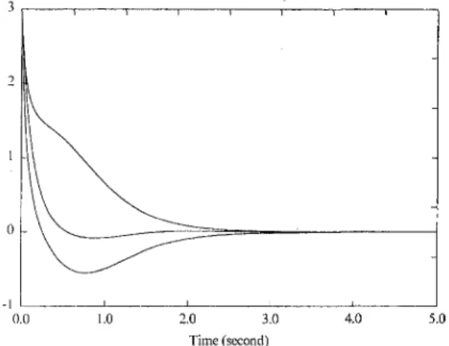
Fig. 1 Time liistory of the system state

2.0 3.0 Time (second)

Fig. 2 Time history of the control inputs

the proposed forward differential Riccati equation is guaranteed by Lemma 4 below (P(t) < 72/).

Before the analysis of the closed-loop system stability under the proposed control (18), one needs the following lemmas regarding the properties of the transformed system matrices A(t) and B(t). The first lemma shows that (A(t), B(t)) is ''uniformly controllable" in the sense that its "controllability grammian" as defined in Definition 2 is uniformly strictly positive definite. Lemma 2: If the pair (A(r), B{t)) in Eq. (1) is uniformly controllable, the pair (A(r), B{t)) in Eq. (13) is also uniformly controllable in the sense of Definition 2.

Proof: See Appendix.

The second lemma, whose proof is omitted, is an immediate consequence of Lemma 2 and Duality (Callier and Desoer,

1992).

Lemma 3: Under the Hypothesis of Lemma 2, the pair (-A^(t), B^(t)) is uniformly observable in the sense of Defi-nition 1.

Observe that the differential Riccati Equation (17) can be re-written as

Pit) = {-A\t))P(t) + P{t){~A\t)Y

+ R,{t) - P{t){B\t)YR-2\t){B\t))P{t), (19) which has exactly the same form as the observer Riccati Equa-tion (5) in SecEqua-tion 2. Therefore, based on Lemma 3, one can follow the procedure in proving Lemma 1 to show that P{t) in Eq. (17) is uniformly bounded above and below.

Lemma 4: Under the Hypothesis of Lemma 2, there exist positive constants yj and 72 such that the solution P(f) of the Riccati Eq. (17) satisfies

7 i / r a P{t) < 72/, Vr > 0.

One can now state the main theorem of this paper, which shows that the proposed control (18) is globally stabilizing for the system ( 1 ) .

Theorem 2: Consider the system (1) and the state feedback control (18) and (17). If the system (1) is uniformly controlla-ble, the closed-loop system is globally exponentially stable.

Proof: In this proof, one first shows that the transformed input v ( 0 in Eq. (16) drives the tran,sformed state z(f) to infin-ity exponentially. Choose a function V{t, z) = z^(t)P(t)z(t). It follows from Lemma 4 that

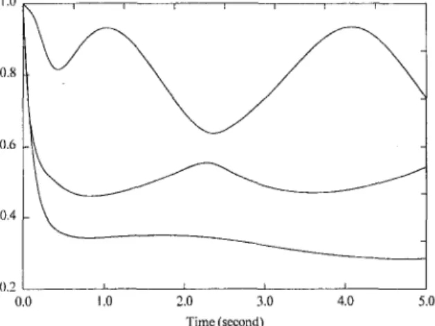
Fig. 3 Singular values of P ( 0

Calculating the time derivative of V(t, z) along the solutions of Eqs. (13), (16), and (17) yields

V = z'iA'' + K'B'^)Pz + z''P(A + BK)z

+ z''(-A''P - PA + R2- PSR;'B'^P)Z

= z'R^z + z^PBR^'B^'Pz a z'RtZ. (21) Assuming that R[(t) > al for some positive constant a, one obtains

V(t,z) s a\\zO)fs. — V(t,z),

where Eq. (20) is used to obtain the second inequality, which suggests that V(t, z) approaches infinity exponentially. It then follows from Eq. (20) that z(t) also approaches infinity expo-nentially. Finally, one concludes from Eq. (8) that x(t) ap-proaches zero exponentially. Q.E.D.

To verify the effectiveness of the proposed state feedback control, a simulation example is given below.

Example: Consider a multivariable time-varying system (1) with

A(t) =

-1-I-1.5 cos^f 1 - 1.5 sinf c o s ; - 1 - l.Ssinrcosr - l + 1.5sin^f 0 -sin t 1 -5 -f sin ? 5 ( 0 = 1 2 3 1 0 1

The initial condition of the system isx'^(O) = [3, 3, 3 ] . From simulation studies, it is found that the open-loop system is unstable. The proposed control (18) is then applied to the sys-tem with the following design parameters P ( 0 ) = /, Riit) = / and R2(t) = / in Eq. (17). Figure 1 shows the time history of the system state, which converges to zero as guaranteed by Theorem 2, and Fig. 2 shows the time history of the control inputs. In this simulation, the P(t) matrix is calculated by on-line integrating the forward differential equation (17) starting from t = 0. The integration is performed by using a finite difference approximation for the differential operator with a time step At = 0.01 second. The calculated singular values of P{t) are plotted in Fig. 3. One interesting question is the relationship between the state convergence rate and the design matrices R\(t) and RzU) in Eq. (17). It may appear from Eq. (21) that a larger Ri{t) and a smaller R2(t) will result in a faster divergent rate of V{t, z), and hence a faster convergent

rate of the system state x(t). However, the exact relationship is to be further studied in the future.

4 Conclusions

A new design is proposed in this paper for the state feedback control of multivariable linear time-varying systems. The new design is based on an inversion state transformation and a for-ward differential Riccati equation. Such a new design results in a time-varying nonlinear dynamic state feedback control law with the control input depending only on past and present infor-mation of the system matrices. In conventional time-varying LQ control, where a backward differential Riccati equation is used, the control input depends on future information of the time-varying system matrices, which is difficult to predict in most practical situations.

Acknowledgment

This work was supported by the National Science Council of the Republic of China under grant number NSC-85-2212-E-002-001.

References

Anderson, B. D. O., and Moore, J. B„ 1968, "Extensions of Quadratic Minimi-zation Theory, II. Infinite Time Results," Int. J. Control, Vol, 7, pp. 473-480. Arvanitis, K. G., and Paraskevopoulos, P. N., 1992, "Uniform Exact Model Matching for a Class of Linear Time-Varying Analytic Systems," System.'^ and

Control Letters, Vol. 19, pp. 312-323.

Callier, F., and Desoer, C. A., 1992, Linear System Theory, Springer-Verlag, Hong Kong.

Chen, C. T., 1984, Linear System Theory and Design, Holt, Rinehart and Win-ston, New York,

Kalman, R. E„ 1964, "When Is a Linear Control System Optimal," ASME

Journal of Basic Engineering, pp. 51 - 6 0 .

Kalman, R. E„ and Bucy, R. S., 1961, "New Results in Linear Filtering and Prediction Theory," ASME Journal of Basic Engineering, pp. 95-108.

Kwakernaak, H,, and Sivan, R., 1972, Linear Optimal Control Systems, Wiley, New York,

Rugh, W. J„ 1993, Linear System Theory, Prentice-Hall, Englewood Cliffs, NJ, Valasek, M,, and Olgac, N,, 1993, "Generahzation of Ackermann's Formula for Linear MIMO Time Invariant and Time Varying Systeins," Proceedings of

Conference on Decision and Control, pp. 827-831,

Wolovich, W, A„ 1968, "On the Stabilization of Controllable Systems," IEEE

Trans. Automat. Contr., Vol, 13, pp, 569-572,

Wonham, W. M., 1968, "On a Matrix Riccati Equation of Stochastic Control,"

SIAM J. Control, Vol, 6, pp, 681-697.

A P P E N D I X

Proof of Lemma 2: The purpose is to prove that there exists a positive constant a such that the "controllability grammian" of (A(r), B(t)) satisfies the lower bound:

Tit) = $ ( ? , T ) B ( T ) 5 ' ' ( T ) $ ^ ( f , T)dT > a / > 0, where $(f, r ) is defined by

'"'^''^^^Aitmur)

By direction differentiation, it can be verified that any z(t) satisfying the following integral equation also satisfies the dif-ferential Eq. (13)

Z ( r ) = $ ( f , ? o ) z ( f o ) + I Ht,T)B(T)v(T)dT, ( A 5 )

' ' ' 0

From the Hypothesis of the Lemma, the original system (1) is uniformly controllable. It then follows from the definition of uniform controllable (Callier and Desoer, 1992) that for the system (1), given any bounded and nonzero Xo, X/and any time instant t, there exist a constant A > 0 with A independent of t, and a bounded control input M* defined on the time interval [t - A, t], such that u* drives the system (1) from x{t - A ) = Xo tox(t) = Xf. Next observe that the inversion transformation from X to z in Eq. (7) and that from « to u in Eq. (10) are injective for all x * 0; hence, the same statement can be said about the transformed system (13); that is, given any bounded and nonzero zo, Z; and any time instant t, there exist a constant A > 0 with A independent of t, and a bounded transformed control input v* defined on the time interval [f - A, ?], such that D* drives the transformed system (13) from z(t — A ) = Zo to z(f) = Z/.

One can now prove Eq. ( A l ) by a contradiction argument using the above statement and Eq. (A5). Assume that Equation ( A l ) does not hold; in other words, there exist sequences of time instants f;'s, positive constants a,'s and unit vectors h\s e /?", with lim,-oo ti = «> and

lim a, = 0, (A6)

such that

hjl(t,)h, = a,..

Denote hj^(ti, T)B(T) = FJ{T). The above equation becames hjKti)hi (T)Fi(T)dT = « ; .

Since FjF, is always non-negative, one concludes from Eq. (A6) that

lim FJ(T) = lim hj$(ti, T)B{T) = 0, ('-•CO i^xa

Vr G [r, - A, ; , ] . (A7) Following the last statement in the previous paragraph, there exists a bounded transformed control input vf that drives z(f, - A) = $(f, - A, t,)hi/2 to z(ti) = /!,-. The integral Eq. (A5) (with t = ti and to = ti - A) thus becomes

hi/2

£

x(ti-A) = $ ( A - A , f , ) / ! , / 2 t o x{ti) • hi (A9) \mti-A,ti)hi/2r ii»,-ii Since the differential equation (A2) for $ ( ; , T ) is linear with bounded coefficients (recall that A(t) is uniformly bounded as long as x * 0), it is easy to show that there exist two positive constants m\ and m2 so that

0 < m, =s (Tj[$(A - A, f,)] s: mj, V/, (AlO) where aj denotes the singular value of a matrix. Equation (AlO) then suggests that both \\x(ti - A)|| and ||x(f,)|| in Eq. (A9) are uniformly bounded, and they are also uniformly bounded away from zero. Consequently, the control input uf that drives the system from x(ti - A ) to x(f,) is also uniformly bounded with respect to / (see Eq. (C-1) in Appendix C of Chen, 1984). Without loss of generality, assuming that \\x(t)\\ > e for some small number e > 0 during the motion when it is transfered from x(ti - A ) to x(f,). It then follows from Eq. (10) that the transformed input vf, which transfers z(f, - A ) to z(f,), is also uniformly bounded with respect to i\ i.e.,

\\vf(T)\\:sM<^, V T G [f, - A, f,], and Vi, ( A l l ) Now, multiplying both sides of Eq. (AS) by hj gives

hJh,/2= \ hJ^(ti,T)B(x,T)vf(T)dT. J I;- A

^{;

However, according to Eqs. (A7) and ( A l l ) , the right-hand side of the equation approaches zero as ( approaches infinity, meaning that

lim||/!,||V2 = 1 / 2 = 0.

The above contradiction proves that /(f) in Eq. ( A l ) will not approach singular asymptotically, and therefore remains uni-formly positive definite. Q.E.D.