行政院國家科學委員會專題研究計畫 期中進度報告
線上基因演算之模糊類神經網路及其在非線性系統辨識與
控制之應用(1/2)
計畫類別: 個別型計畫
計畫編號:
NSC91-2213-E-030-002-執行期間: 91 年 08 月 01 日至 92 年 07 月 31 日
執行單位: 輔仁大學電子工程學系(所)
計畫主持人: 王偉彥
計畫參與人員: 林炳榮、陳冠銘、張貞觀、郭重佑
報告類型: 精簡報告
處理方式: 本計畫可公開查詢
中
華
民
國 92 年 5 月 21 日
線上基因演算之模糊類神經網路及其在非線性系統辨識與控制之應用
(1/2)
On-line Genetic Algorithm for Fuzzy-Neural Network and Its Applications
in Nonlinear System Identification and Control
計畫編號:NSC 91-2213-E-030-002 執行期限:91 年 8 月 1 日至 92 年 7 月 31 日 主持人:王偉彥 輔仁大學電子工程系 參與人員:林炳榮、陳冠銘、張貞觀、郭重佑 輔仁大學電子工程系 摘要 本計畫提出一種以基因演算為基礎輸出回授直接適應性模糊類神經控制器的設計法則,此控制器 用以控制具未確定項之非線性動態系統。吾人使用一種 reduced-form genetic algorithm (RGA)去調 整模糊類神經控制器的權重因子,使得直接適應性模糊類神經控制器的權重因子可以基因演算方 式線上調整。線上調整的適應函數是使用 Lyapunov 設計方法推導。最後,加入監督式控制器確 保控制系統的穩定性。
Abstr act
In this project, we propose a novel design of a GA-based output-feedback direct adaptive fuzzy-neural controller (GODAF controller) for uncertain nonlinear dynamical systems. The weighting factors of the direct adaptive fuzzy-neural controller can successfully be tuned on-line via a GA approach. We use a reduced-form genetic algorithm (RGA) to adjust the weightings of the fuzzy-neural network. A new fitness function for on-line tuning the weighting vector of the fuzzy-neural controller is established by the Lyapunov design approach. A supervisory controller is incorporated into the GODAF controller to guarantee the stability of the closed-loop nonlinear system.
Keywords: genetic algorithms, fuzzy neural networks, function approximation, direct adaptive control, and supervisory control.
I. Intr oduction
Since neural networks and fuzzy logic systems are universal approximators, they have been widely used to approximate nonlinear functions for many practical applications [3]. Traditionally, fuzzy logic systems or/and neural networks [1]-[5] are trained by using gradient-based methods, which may fall into a local minimum during the learning process. Such techniques also suffer from difficulties such as the choice of starting guess, convergence, etc. Moreover, since the cost function generally has multiple local minima, the attainment of the global optimum by these nonlinear optimization techniques is difficult [6]. Genetic algorithms (GAs) [7]-[12], with their capabilities of directed random search for global optimization, have drawn significant attention in various fields. Thanks to a probabilistic search procedure based on the mechanics of natural selection and natural genetics, genetic algorithms are highly effective and robust over a broad spectrum of problems [13]-[15], [28]-[29], including parameter estimation [13], robust stability analysis [28], and controller design [29]. The use of genetic algorithms to overcome the problems encountered by conventional learning methods for fuzzy-neural networks had been proposed in [16]-[18]. In this project, a reduced-form genetic algorithm (RGA) [27] is adopted to tune the adjustable parameters (weightings) of a fuzzy-neural network.
Recently, some adaptive fuzzy-neural control systems [19]-[23], [30] have been proposed to incorporate expert information systematically, and their stability can be guaranteed by the universal approximation theorem [2], [5], [21]. Theoretical justification on the use of the direct adaptive fuzzy controllers in [5] using a state feedback approach is valid when all of the system states are available for measurement. In practice, however, the state feedback control does not always hold because system states are not always available. Estimations of states from the system output for output feedback control design of the direct adaptive fuzzy-neural controller are required. Thus far, the problem as to how a direct adaptive fuzzy-neural output-feedback controller is designed remains to be solved.
In this project, we propose a GA-based output-feedback direct adaptive fuzzy-neural controller (GODAF controller) for uncertain nonlinear dynamical systems. The weighting vector of the GODAF controller can be successfully tuned on-line via the RGA approach, instead of solving complicated mathematical equations. A new fitness function for on-line tuning the weighting vector of the fuzzy-neural controller is established by the Lyapunov design approach. In addition, a supervisory controller [5], [23] is incorporated into the GODAF controller to guarantee the stability the closed-loop nonlinear system. If the closed-loop system controlled by the GODAF controller becomes unstable,
especially in the transient period, the supervisory controller will be activated to work with the GODAF controller to stabilize the closed-loop system. On the other hand, if the GODAF controller works well, the supervisory controller will be deactivated.
II. Fuzzy-Neur al Networ ks
Fuzzy-neural networks are generally a fuzzy inference system constructed from structure of neural network. Learning algorithms are used to adjust the weightings of the fuzzy inference system.
Given the input data xq,q=1,2,L,n, and the output data yp,p=1,2,L,m, the ith fuzzy rule has the following form [31]-[34]: i m m i i n n i i w y and w y THEN A is x and A is x IF R = = L L 1 1 1 1 : (1)
where i is a rule number, i q
A ’s are the fuzzy sets of the antecedent part, and i p
w are real numbers of
the consequent part. When the inputs T n
x x x
x=[1 2L ] are given, the output ypof the fuzzy inference
can be derived from the following equations:
ϕ µ µ T p h i q A n q h i q A n q i p p p w x x w w x y i q i q = ∏ ∏ = ∑ ∑ = = = = 1 1 1 1 )) ( ( )) ( ( ) ( (2) where Ai(xq) q
µ is the membership function of Aqi , h is the number of the fuzzy rules,
T h p p p p w w w
w =[ 1 2L ] is a weighting vector related to the pth output yp(x), and ϕ=[ϕ1ϕ2Lϕh] is a set of fuzzy basis functions defined as:
. , , 2 , 1 , )) ( ( ) ( ) ( 1 1 1 h i x x x h i n q q A n q q A i i q i q L = = ∑ ∏ ∏ = = = µ µ ϕ (3)
By adjusting weighting values
w
ip of the fuzzy-neural network, w=[w1TwT2LwTm]T is a weighting vector of the fuzzy-neural network for m outputs, and the size of the weighting vector w is α=m×h.III. GA-Based Lear ning of Weighting Vector s of Fuzzy-Neur al Networ ks
In this project, the reduced-form genetic algorithm (RGA) in [27], characterized by three simplified processes is proposed, which evolutionarily obtains the optimal weighting vector for the fuzzy neural network.
A. Population Initialization
Assume that the weighting vector w of the fuzzy-neural network is a chromosome that represents a potential solution to the problem and is defined as:
h m R w w w w w w w w w w w w w T h m m m h h T m T T × = ∈ = = α α, ] [ ] [ 2 1 2 2 2 1 2 1 2 1 1 1 2 1 L L L L K (4)
where wij , defined in (2), is a weighting chosen from within the pre-defined interval
R w w
D=[ min, max]⊆ .
The initial chromosomes are randomly generated from within the feasible range D. A population with k chromosomes as defined in (4) is represented as:
= = Ψ + + + k k k k k 1 2 1 1 1 2 1 2 2 2 2 1 1 1 2 1 1 2 1 α α α α α α φ φ φ φ φ φ φ φ φ φ φ φ φ φ φ M L M O M M L L M (5)
where φl=[wTφαl+1]=[φ1lφ2lLφαlφαl+1] is the thl chromosome, l=1,2,K,k. Each chromosome, being a weighting vector w of the fuzzy-neural network, has α+1 elements and is a candidate of the population. φαl+1 is defined as a virtual gene, on which single gene crossover does not affect the
fitness values of the population, if the crossover point chooses j=α. The single gene crossover will be introduced later. It is expected that one of the candidate solutions, φl, can be evolutionarily obtained to form a set of near-optimal parameters for the fuzzy-neural network. Note that the number of chromosomes, k, needs be an even number and larger than 3 as required by the single gene crossover method below.
After initialization, two genetic operations: crossover and mutation are performed during procreation.
B. Fitness function
The performance of each chromosome is evaluated according to its fitness. After some number of generations of evolution, it is expected that the genetic algorithm converges and a best chromosome with largest fitness (or smallest error) representing the optimal solution to the problem is obtained.
C. Single Gene Cr ossover
In order to deal with adjustable parameters, the single gene crossover [27] is introduced into the learning algorithm.
D. Sor ting
After crossover, the newly generated population is sorted by ranking the fitness of chromosomes within the population. The first chromosome of the sorted population has the highest fitness value (or smallest error).
E. Mutation
After sorting, the first chromosome is the best one in the population in terms of fitness. The mutation operator in [27] is employed as
≤ − ∆ − > − ∆ + = + , 5 . 0 if ) , ( , 5 . 0 if ) , ( ˆ min 1 1 1 max 1 ) 1 2 / ( δ φ φ δ φ φ φ w t w t j j j j k j (6) ∆(t,y)=y*γ*(1−t/T)γ , (7)
where δ∈[0,1] is a random value,t is the current iteration, γ is a random number from [0..1], and T
is the maximal generation number.
IV. GA-Based Output-Feedback Dir ect Adaptive Fuzzy-Neur al Contr oller s A . System For mulation
Consider the nth order nonlinear dynamical system of the form
1 2 1 2 1 1 3 2 2 1 ) , , , ( ) , , , ( f x y d u x x x g x x x x x x x x x x n n n n n = + + = = = = − K K & & M & & (8)
where d is the external bounded disturbance, u∈R is the control input and y∈R is the system output. We assume that f and g are uncertain functions, and g is, without loss of generality, a strictly positive function. It is also assumed that a solution for (8) exists. In addition, only the system output y is assumed to be measurable. The control objective is to design a GA-based output-feedback direct adaptive fuzzy-neural controller (GODAF controller) such that the system output y follows a given bounded reference signal ym.
First, we convert the tracking problem to a regulation problem. Equation (8) can be rewritten as
) ) ( ) ( f ( +g u+d + =Ax B x x x& , x CT y= , (9) where = 0 0 0 0 0 1 0 0 0 0 1 0 0 0 0 1 0 L L L L L L L L A , = 1 0 0 0 M B , = 0 0 0 1 M C ,
and x=[x,x&,...,x(n−1)]T =[x1,x2,...,xn]T∈Rn is a vector of states. Define the output tracking error y
y
e= m− , the reference vector ym=[ym,y&m,K,y(mn−1)] and the tracking error vector e=[e,e&,...,e(n−1)]T T n e e e, , , ] [1 2K = .
Based on the certainty equivalence approach, an optimal control law is [ f( ) ˆ] ) ( 1 ( ) * x K e x T c n m y g u = − + + (10)
where eˆ=ym−xˆ, eˆ and xˆdenote the estimates of e and x, respectively. Kc=[kncknc−1...k1c]T is the feedback gain vector, chosen such that the characteristic polynomial of T
c
BK
A− is Hurwitz because
) ,
) (x
g are assumed to be uncertain, the optimal control law (10) cannot be implemented. To overcome this problem, suppose a control input u is
d
f u
u
u= + (11)
where uf is a fuzzy-neural controller designed to approximate the optimal control law (18), and the control term ud is employed to compensate for the external disturbance and the modeling error. From (9), (10) and (11), we have
. ] ) ( ) ( ) ( [ ˆ 1 * e C x x x B e BK Ae e T d f T c e d u g u g u g = − − − + − = & (12)
Thus, the tracking problem has been converted into a regulation problem of designing a state observer for estimating the state vector e in (12) in order to regulate e1 to zero.
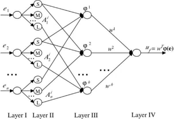
In addition, the configuration of the fuzzy-neural network is shown in Fig. 1. The fuzzy inference engine uses the fuzzy IF-THEN rules to perform a mapping from an input linguistic vector
[
]
n n R e e e ∈ = 1, 2,...,e to an output linguistic variable uf ∈R. The ith fuzzy IF-THEN rule is written as Ri: If e1 isA1i and
… and en is i n
A than uf isBi, (13)
where A1i,A2i,...,Ain and Bi are fuzzy sets. By using product inference, a singleton fuzzifier, and a
center-average defuzzifier, the output of the fuzzy-neural network in Fig. 1 can be expressed as
) ( ) ( ) ( ) ( 1 1 1 1 e e ϕ µ µ T h i n j j A h i n j j A i f w e e w w u i j i j = = ∑ ∏ ∑ ∏ = = = = (14) where Ai(ej) j
µ is the membership function value of the fuzzy variable, h is the total number of the IF-THEN rules , wi is the point at which ( i)=1
Bi w
µ , w=[w1,w2,...,wh]T is an adjustable weighting
vector which is tuned by the RGA, andϕ=[ϕ1,ϕ2,...,ϕh]T is a fuzzy basis vector, where ϕi is defined as (3).
When the inputs are given to the fuzzy-neural network shown in Fig. 1, the truth value ϕi(layer III) of
the antecedent part of the ith implication is calculated by (3). At layer IV, the output stands for the value of uf(ew).
B . Design of the GODAF Contr oller
First, we replace uf in (11) by the output of the fuzzy-neural network, i.e.,
) ˆ ( ) | ˆ (e Tϕe f w w u = (15) where eˆ denotes the estimate of e.
Next, consider the following observer that estimates the state vector e in (12)
e C K B e BK e A e ˆ ˆ ) ˆ ( ) ( ˆ ˆ ˆ 1 1 1 T o d T c e e e gu gv = − + − + − = & (16)
where Ko =[k1o,k2o,...,kno]T is the observer gain vector, chosen such that the characteristic polynomial
of T
oC
K
A− is strictly Hurwitz because (C,A) is observable. The control term v is employed to compensate the external disturbance d and the modeling error. We define the observation errors as
e e e ˆ ~= − and 1 1 1 ˆ ~ e e
e = − . Subtracting (16) from (12), we have
. ~ ~ ] ) | ˆ ( [ ~ ) ( ~ 1 C e e B e C K A e T f T o e d gv w gu gu = − − − + − = ∗ & (17)
Besides, the output error dynamics of (17) can be given as
] ) | ˆ ( )[ ( ~ 1 H s gu gu w gv d e = ∗− f e − − (18)
where s is the Laplace variable, and H(s)=CT(sI−(A−KoCT))−1B is the transfer function of (18). In order to adopt the RGA, we assume that the optimal weighting vector w∗ exists.
Assumption 1 [24]:
priori that the optimal parameter vector arg min[ sup (ˆ| )] ˆ ,ˆ w u u w U U M w w e e ee e − = ∗ ∈ ∈ ∈
∗ lies in some convex region
{ n w}
w w w m
M = ∈ℜ : ≤ , where the radius mw is constant. ♦
According to assumption 1, (17) can be rewritten as
e C e e B e C K A e ~ ~ ] ) | ˆ ( ) | ˆ ( [ ~ ) ( ~ 1 T f f T o e d gv w gu w gu = − + − − + − = ∗ δ & (19)
where δ=gu∗−guf(eˆ|w∗) is an approximation error. According to (15), (19) can be rewritten as
e C e B e C K A e ~ ~ ] ) ˆ ( ~ [ ~ ) ( ~ 1 T T T o e d gv w g = − + − + − = ϕ δ & (20)
where w~=w∗−w. Since only the output ~e1 in (20) is assumed to be measurable, we use the
SPR-Lyapunov design approach [25] to analyze the stability of (20). Equation (20) can be rewritten as
] ) ˆ ( ~ )[ ( ~ 1 H s gw gv d e = Tϕ e − +δ− (21)
where H
( )
s =CT(sI−(A−KoCT))−1B is a known stable transfer function. In order to employ the SPR-Lyapunov design approach, (21) can be written as] ) ˆ ( ~ )[ ( ) ( ~ 1 H sLs wT vf f e = ϕe − +δ (22)
wherevf=L−1(s)[gv],δf=L−1(s)[δ−d+gw~Tϕ(ˆe)]−w~Tϕ(eˆ), and L(s) is chosen so that L−1(s) is a proper stable transfer
function and H(s)L(s) is a proper SPR transfer function. Suppose that
m m m m bs b s b s s
L( )= + 1 −1+ 2 −2+...+ , where m<n, such that H(s)L(s) is a proper SPR transfer function. Then the state-space realization of (22) can be written as
e C e B e A e ~ ~ ] ) ˆ ( ~ [ ~ ~ 1 Tc f f T c c e v w = + − + = ϕ δ & (23) where n m T c n n T o c=(A−K C )∈ℜ × ,B =[00Lb1b2Lb ]∈ℜ A and CTc =[10L0]∈ℜn.
For the purpose of stability analysis of the GODAF controller, the following assumptions and lemma are required.
Assumption 2: The uncertain nonlinear function g(x) is bounded by
2
1 ( ) β
β ≤ gx ≤ (24)
where gl=β1,gu=β2 are given positive constants. The uncertain nonlinear function f(x) is bounded
by f(x)≤fu(xˆ). ♦
Assumption 3: δf is assumed to satisfy
ε
δf ≤ (25)
where ε is a positive constant. ♦
Consider the Lyapunov function candidate
e P e ~ ~ 2 1 T V= , ( 2 6 )
where P=PT>0. Differentiating (26) with respect to time and inserting (23) in the above equation yield ] ~ [ ~ ~ ) ( ~ 2 1 f f T c T c T c T w v V&= e A P+PA e+e PB ϕ− +δ ( 2 7 )
Because H(s)L(s) is SPR, there exists P=PT>0 such that
c c c T c C PB Q PA P A = − = + ( 2 8 )
where Q=QT >0. By using (28), (27) becomes
] ~ [ ~ ~ ~ 2 1 1 T f f T e w v V&=− e Qe+ ϕ− +δ . Let vbe given as < − ≥ = 0 ~ if 0 ~ if 1 1 e e v ρ ρ (29) where 1 β ε
ρ≥ . By using assumptions 2 and 3, (29) and the fact min 12 2 min(Q)~e λ (Q)~e λ ≥ , where 0 ) ( min Q > λ , we have
ϕ λ e e wT V ( )~ ~~ 2 1 1 2 1 min + − ≤ Q & . ( 3 0 ) Since w~=w∗−w, we have ϕ ϕ λ e ew ew V 1 1 2 1 min( )~ ~ ~ 2 1 + − − ≤ Q ∗ & (31) f u e u e e 1 1 2 1 min( )~ ~ ~ 2 1 − + − ≤ λ Q ∗ (32)
However, from (32) we see that it is very difficult to make the uf such that the last term of (32) is less than zero. How can this problem be solved?
First, we use RGA to tune the weightings of uf in hope that the last term of (32) is less than zero. Since u* is unknown, we need to find a new fitness function without u* for on-line tuning such that
0
<
V& is satisfied. Using assumption 2 and (10), (32) can be rewritten as
+ + + + − ≤ f T c n m u l u y f g e e V e K x x Q ˆ ) ˆ ( ) ( 1 ~ ~ ) ( 2 1 ) ( 1 2 1 min λ & (33)
We define a new fitness function without
u
* and for on-line tuning as0 ) ˆ ( ˆ ) ˆ ( ) ( 1 ~ ~ ) ( 2 1 ) ( ) ( 1 2 1 min < + + + + − = w u y f g e e w fitness f T c n m u l e e K x x Q λ (34)
(34) guarantees that V&<0 . For using the RGA to tune the weightings of uf , the sequential-search-based crossover point (SSCP) method determines a better crossover point j based on the fitness function (34) before the single gene crossover actually takes place. That is, a new generation of weightings is obtained by the single gene crossover if (34) is checked and satisfied. If there is no satisfactory crossover point in the current generation, then the crossover point is designated as j=α, so that the single gene crossover is performed on the virtual gene, and the fitness values will not be affected. In addition, after crossover, the generated population is sorted by ranking the fitness of chromosomes within the population, resulting in fitness(φˆ1)≤fitness(φˆ2)L≤ fitness(φˆk) . The first chromosome φˆ1 of the sorted population Ψˆ=[φˆ1φˆ2Lφˆk]T has the smallest fitness value.
However, there are two situations where the fitness function (34) is not satisfied. One situation is no crossover point satisfying (34). The other situation is that in the initial searching of the RGA, a random set of weightings in RGA will result in a large approximation error between uf and u*. We
solve this problem by appending a supervisory control term us to uf . That is, the controller becomes
uc=uf +us. (35)
This additional control term
u
s is called a supervisory control [5], [23]. Then using (32), we have) ( ~ ~ ) ( 2 1 1 2 1 min e e u uf us V&≤− λ Q + ∗− − s f eu u u e e 1 1 2 1 min( )~ ~( ) ~ 2 1 + + − − ≤ λ Q ∗ . (36)
By using (4-3) and assumption 2, we have
s f T c n m u l u e u y f g e e V 1 ) ( 1 2 1 min ~ ˆ ) ˆ ( ) ( 1 ~ ~ ) ( 2 1 − + + + + − ≤ e K x x Q λ & (37)
Then, we construct the supervisory control us as follows:
+ + + ∗ = x K e x ˆ ) ˆ ( ) ( 1 ) ~ sgn(1 u (mn) Tc l f s f y g u e I u (38)
where I=1 if V>V>0 (which is a constant specified by the designer), and I=0 if V≤V. V
denotes an error threshold and should be as small as possible. Because of I, the us is a supervisory kind of controller. Substituting (38) into (37) and considering the I=1 case, we have
0 ~ ) ( 2 1 2 1 min ≤ − ≤ Q e V& λ . (39)
Equation (39) only guarantees that e~1(t)∈L∞ and ~e(t)∈L∞, but does not guarantee convergence.
Because all variables in the right-hand side of (23) are bounded, e&~1(t) is bounded, i.e., e~&1(t)∈L∞.
Integrating both sides of (39) and some manipulation yields
) ( 2 1 ) ( ) 0 ( ) ( ~ min 0 2 1 Q λ ∞ − ≤ ∫∞e t dt V V . (40)
Since the right side of (40) is bounded, so ~e1(t)∈L2. Using Barbalat’s lemma [26], we have 0 ) ( ~ lim 1 = ∞ → e t t .
Lemma 1 [25]: Consider the linear time-invariant system
0 ) 0 ( ), ( ) ( ) ( Ax Bu x x x&t = t + t =
where x∈ℜn,u(t)∈ℜm,A∈ℜn×n,B∈ℜn×m. Suppose that A is a Hurwitz matrix andu(t)∈L2e. Let α0
and λ0 be positive constants that satisfy eA( )t−τ ≤λ0e−α0( )t−τ . Then for any constant ξ∈[0,ξ1], where 0 1 2 0<ξ < α , ξ α ξ α λ λ 2 0 0 0 0 2 ) ( 0 t t e t x B u x − + ≤ − ♦
Next, consider (20). Define u=gw~Tϕ )(eˆ−gv+δ−d. Because T oC
K
A− is a Hurwitz matrix, and
u
is bounded under assumptions 1-3, we haveξ α ξ α λ λ 2 0 0 0 2 ) 0 ( ~ ) ( ~ 0 t t u e t − + ≤ − e B e , (41)
according to Lemma 1. Therefore ~e(t)∈L∞. Using (16) and ud =v, we obtain
. ˆ ˆ ~ ˆ ) ( ˆ 1 C e e C K e BK A e T T o T c e = + − = & (42) Similarly, because T c BK
A− is a Hurwitz matrix and ~e(t) is bounded, eˆ(t) is bounded. From e~=e−eˆ, it follows that e1,e∈L∞ and e1(t)→0 as t→∞. From e,ˆe∈L∞, it follows that x ˆ,x∈L∞ . The
boundedness of y(t) follows that of e1(t) andym(t).
Therefore, we conclude that the nonlinear system (15) satisfies assumptions 1-3 and the total control law is d s f w u u u u= (eˆ| )+ + (43)
with the state observer (16) and the RGA with the fitness function in (34). Then all signals in the closed-loop system are bounded, and e1(t)→0 as
t
→
∞
.V. Simulation Results
Example 1: Consider the Duffing forced oscillation system
. cos 12 1 . 0 1 3 1 2 2 2 1 x y d u t x x x x x = + + + − − = = & &
It is assumed that the external disturbance d(t) is a square wave having an amplitude ±1 with a period of 2π. The control objective is to control the state x1 of the system to track the reference
trajectory ym, under the condition that only the system output
y
is measurable. The designparameters are selected as V=0.005, ρ=50, D=[−10,10], and Q=diag[500500]. The population size is 4, and the mutation rate is pm=(1−t T)×0.05+0.05, where t is the current iteration and T is the maximal generation number. The feedback and observer gain vectors are given as T
c=[14424]
K and
T o=[60900]
K , respectively. The filter L−1(s) is given as L−1(s)=1(s+2). The initial states are chosen to be x1(0)=3,x2(0)=3,xˆ1(0)=−1,xˆ2(0)=−1 and eˆ(0)=ym(0)−xˆ(0). Simulation results are provided for
two cases with different reference trajectories, i.e.,ym=0 (Case 1), ym=sint (Case 2)。
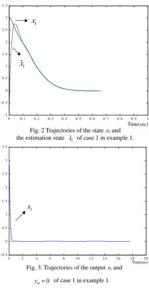
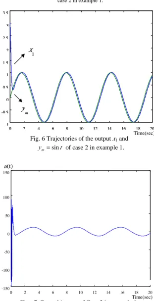
As shown in Figs. 2 (case 1) and 5 (case 2), the trajectory of the estimation state xˆ1 catches up to the
trajectory of the system state x1 very quickly and well for case 1 and case 2, respectively. Moreover,
the tracking performance is good as shown in Fig. 3 (case 1) and Fig. 6 (case 2), in which ym is the reference trajectory andx1is the system output. As shown in Figs. 4 (case 1) and 7 (case 2), a chattering
effect on the control input (due to ud+us) for these cases appears in the initial searching. In this period, the RGA searches the neighborhood for the optimal parameters of the GODAF controller. After this initial searching, the RGA has almost found the optimal parameters and the chattering effect on the control input (due to ud+us) disappears.
VI. Conclusions
This project proposed a reduced-form genetic algorithm (RGA), which can be successfully applied to the fuzzy-neural network to search for optimal weightings. A GA-based output-feedback direct adaptive fuzzy-neural controller (GODAF controller) was also proposed. The weighting vector of the direct adaptive fuzzy-neural controller can be successfully tuned on-line via the RGA approach, instead of solving complicated mathematical equations. Moreover, a new fitness function for on-line tuning the weighting vector of the fuzzy-neural controller is established by the Lyapunov design approach. The GODAF controller with the supervisory controller guarantees the stability of the resulting closed-loop system.
Refer ences
[1] K. Hornik, M. Stinchcombe, and H. White, "Multilayer feedforward networks are universal approximators," Neural Networks, no. 2, pp. 359-366, 1989.
[2] L.X. Wang and J.M. Mendel, "Fuzzy basis functions, universal approximation, and orthogonal least squares learning," IEEE Trans. on Neural Networks, vol. 3, no. 5, pp. 807-814, 1992.
[3] Fei-Yue Wang, "Building Knowledge Structure in Neural Nets Using Fuzzy Logic," Robotics and Manufacturing: Recent Trends in Research, Education and Applications, Ed. M. Jamshidi, New York: ASME Press, 1992.
[4] Wei-Yen Wang, Tsu-Tian Lee, Ching-Lang Liu, and Chi-Hsu Wang, “Function Approximation Using Fuzzy Neural Networks with Robust Learning Algorithm,”IEEE Transactions on Systems, Man, and Cybernetics-Part B: Cybernetics, Vol. 27, No 4, p.740-747, 1997.
[5] Li-Xin Wang, “Adaptive Fuzzy Systems and Control, ” Prentice Hall, 1994.
[6] Z. Yang, T. Hachino, and T. Tsuji, “Model reduction with time delay combining the least-squares method with the genetic algorithm,” IEE Proc. – Control Theory Appl., Vol. 143, No. 3, 1996. [7] G. W. Game and C. D. James, “The Application of Genetic Algorithms to the Optimal Selection of
Parameter Values in Neural Networks for Attitude Control Systems,” IEEE Colloquium on High Accuracy Platform Control in Space, pp. 3/1-3/3, 1993.
[8] Rui Ferreira, A. Pecas Lopes, and Tome Saraiva, “A Real Time Approach to Identify Actions to Prevent Voltage Collapse Using Genetic Algorithms and Neural Networks,” Power Engineering Society Summer Meeting, IEEE, Vol. 1, pp255 –260, 2000.
[9] Mitsuo Gen and Runwei Cheng,Genetic Algorithms and Engineering Design, A Wiley-Interscience Publication, John Wiley & Sons, INC.1997.
[10] Z. Michalewicz, Genetic Algorithms + Data Structures = Evolution Programs, Springer-Verlag, 1996.
[11] D. Goldberg, Genetic Algorithms in Search, Optimisation, and Machine Learning, Addison-Wesley, 1989.
[12] D. Lawrence, Handbook of Genetic Algorithms, Van Nostrand Reinhold, 1991.
[13] K. Kristinsson and G. Dumont, “System identification and control using genetic algorithms,”
IEEE Transaction on System Man and Cybernetics, Vol. 22, pp. 1033-1046, 1992.
[14] Antonio Gonzalez and Raul Perez, ”Selection of Relevant Features in a Fuzzy Genetic Learning Algorithm,” IEEE Transactions on Systems, Man, and Cybernetics-Part B: Cybernetics, Vol. 31, No. 3, June 2001.
[15] R. Caponetto, L. Fortuna, S. Graziani, and M. Xibilia, “Genetic algorithms and applications in system engineering: a survey,” Trans. Inst. Meas. Control, Vol. 15, pp. 143-156, 1993.
[16] Chi-Hsu Wang, H.L. Liu, and C.T. Lin, “Dynamic optimal learning rates of a certain class of fuzzy neural networks and its applications with genetic algorithm,” IEEE Transactions on Systems, Man and Cybernetics, Part B, Vol. 31, No. 3, pp.467 –475, June 2001.
[17] C.T. Lin and C.P. Jou,” GA-based fuzzy reinforcement learning for control of a magnetic bearing system,”IEEE Transactions on Systems, Man and Cybernetics, Part B, Vol. 30, No. 2, PP. 276 –289, April 2000.
[18] Wael A. Farag, Victor H. Quintana, and Germano Lambert-Torres,” A Genetic-Based Neuro-Fuzzy approach for modeling and control of dynamical systems,” IEEE Transactions on neural networks, Vol. 9, No. 5, Sept. 1998.
[19] Brown and Harris, "Neurofuzzy adaptive modelling and control", Prentice Hall, 1994.
[20] Y. G. Leu, Wei-Yen Wang, and Tsu-Tian Lee, “Robust Adaptive Fuzzy-Neural Controllers for Uncertain Nonlinear Systems,” IEEE Trans. On Robotics and Automation, Vol. 15, No. 5, pp. 805-817, October 1999.
[21] J. L. Castro, “Fuzzy logical controllers are universal approximators,” IEEE Trans. Syst., Man, Cybern., Vol. 25, pp 629-635, Apr. 1995.
[22] Wei-Yen Wang, M. L. Chan, C. C. Hsu, and Tsu-Tian Lee, “
H
∞ Tracking-Based Sliding Mode Control for Uncertain Nonlinear Systems via an Adaptive Fuzzy-Neural Approach,”IEEE Trans. on System Man and Cybernetics-Part B, Vol. 32, No.4, pp.483-492, Aug. 2002.[23] L. X. Wang, “A Supervisory Controller for Fuzzy Control Systems that Guarantees Stability,”
IEEE Trans. On Automatic Control, Vol. 39, No. 9, pp.1845-1847, 1994.
[24] K. S. Tsakalis and P. A. Ioannou, Linear time-varying systems. Englewood Cliffs, NJ: Prentice-Hall, 1993.
[25] P.A. Ioannou, and J. Sun, Robust Adaptive control. Englewood Cliffs, NJ: Prentice-Hall, 1996. [26] S.S. Sastry and M. Bodson, Adaptive control: stability, convergence, and robustness. Englewood
Cliffs, NJ: Prentice-Hall, 1989.
[27] Wei-Yen Wang, and Yi-Hsum Li, “Evolutionary Learning of BMF Fuzzy-Neural Networks Using a Reduced-Form Genetic Algorithm,”IEEE Trans. on System Man and Cybernetics-Part B, Vol. 33, No.3, June 2003.
[28] Fadali, M., Y. Zhang, and S. Louis, “Robust stability analysis of discrete-time systems using genetic algorithms,” IEEE Trans. on System Man and Cybernetics, pp.1033-1046, 1992.
[29] Hsu, C., K. Tse and C. Wang, “Digital Redesign of Continuous Systems with Improved Suitability Using Genetic Algorithms,” Electronics Letters, 33, No. 15, pp. 1345-1347, 1997.
[30] Tang Nan, Fei-Yue Wang, Frank W. Ciarallo, and Guihe Qin, "Neuro-Fuzzy Networks: Adaptive Fuzzy Modeling and Control," International Journal of Computer and Information Science, Vol. 1, No. 1, pp.1-21, 2001.
[31] H. Nomura, I. Hayashi, and N. Wakami, “A learning method of fuzzy inference rules by descent method,”IEEE International Conference on Fuzzy Systems, pp. 203 –210, Mar. 1992.
[32] C. H. Wang, W. Y. Wang, T. T. Lee, and P. S. Tseng, "Fuzzy B-spline membership function (BMF) and its applications in fuzzy-neural control," IEEE Transactions on Systems Man and Cybernetics, Vol. 25, No. 5, pp. 841-851, May 1995.
[33] A. M. Luciano, and M. Savastano, “Fuzzy identification of systems with unsupervised learning,”
IEEE Transactions on Systems, Man and Cybernetics, Part B, pp. 138-141, Vol. 27, No. 1, Feb. 1997.
[34] Y.P. Huang, T.M. Yu, “The hybrid grey-based models for temperature prediction,” IEEE Transactions on Systems, Man and Cybernetics, Part B,pp. 284-292, Vol. 27, No. 2, April 1997.
Fig. 1 Configuration of a fuzzy-neural approximator.
Layer I Layer II Layer III Layer IV
...
...
... ... ... w1 w2 wh...
u f= wTϕ(e) An i Ai2 Ai 1 ϕ1 ϕ2 ϕh e1 e2 en S M L S M L S M L0 0 . 1 0 . 2 0 . 3 0 . 4 0 . 5 0 . 6 0 . 7 0 . 8 0 . 9 1 -1 -0 . 5 0 0 . 5 1 1 . 5 2 2 . 5 3 3 . 5 1
x
1 ˆx
Time(sec)
0 0 . 1 0 . 2 0 . 3 0 . 4 0 . 5 0 . 6 0 . 7 0 . 8 0 . 9 1 -1 -0 . 5 0 0 . 5 1 1 . 5 2 2 . 5 3 3 . 5 1x
1 ˆx
Time(sec)
Time(sec)Fig. 2 Trajectories of the state x1 and the estimation state xˆ1 of case 1 in example 1.
0 2 4 6 8 1 0 1 2 1 4 1 6 1 8 2 0 -0 . 5 0 0 . 5 1 1 . 5 2 2 . 5 3 3 . 5 1 x
Time(sec)
0 2 4 6 8 1 0 1 2 1 4 1 6 1 8 2 0 -0 . 5 0 0 . 5 1 1 . 5 2 2 . 5 3 3 . 5 1 xTime(sec)
Time(sec)Fig. 3. Trajectories of the output x1 and 0 = m y of case 1 in example 1. 0 2 4 6 8 10 12 14 16 18 20 -150 -100 -50 0 50 100 150 0 2 4 6 8 10 12 14 16 18 20 -150 -100 -50 0 50 100 150 Time(sec)
Fig. 4 Control input u of case 1 in example 1.
0 0 .1 0 .2 0 .3 0 .4 0 .5 0 .6 0 .7 0 .8 0 .9 1 -1 -0 . 5 0 0 .5 1 1 .5 2 2 .5 3 3 .5 1
x
1 ˆx
Time(sec)
0 0 .1 0 .2 0 .3 0 .4 0 .5 0 .6 0 .7 0 .8 0 .9 1 -1 -0 . 5 0 0 .5 1 1 .5 2 2 .5 3 3 .5 1x
1 ˆx
Time(sec)
Time(sec)Fig. 5. Trajectories of the statex1 and the estimation state x of ˆ1
case 2 in example 1. 0 2 4 6 8 10 12 14 16 18 20 -1 -0.5 0 0.5 1 1.5 2 2.5 3 3.5 1
x
m y 0 2 4 6 8 10 12 14 16 18 20 -1 -0.5 0 0.5 1 1.5 2 2.5 3 3.5 1x
m yFig. 6 Trajectories of the output x1 and
t
ym=sin of case 2 in example 1.
Time(sec) 0 2 4 6 8 10 12 14 16 18 20 -150 -100 -50 0 50 100 150
Fig. 7 Control input u of Case 2 in example 1.
Time(sec)