防丟器的剖面追蹤研究 - 政大學術集成

全文

(1)國立政治大學統計學系碩士學位論文. 指導教授: 楊素芬博士蔡紋琦博士. 立. 政治大. ‧ 國. 學. 防丟器的剖面追蹤研究. ‧. Profile Monitoring on the RSSI of Babyfinder. n. er. io. sit. y. Nat. al. Ch. engchi. i Un. v. 研究生：徐伊萱撰中華民國九十九年六月.

(2) 謝. 辭. 時光荏苒，兩年的碩士生涯將在這本論文付梓之刻劃下尾聲，回首這一路走來，滿懷之感謝油然而生。這本論文的完成，得自太多人的幫助，謹以此篇論文獻給這一路來幫助、陪伴我的人。首先感謝我的指導教授，感謝. 楊素芬老師一直以來耐心的指導，對於老. 師付出的心力及平日的關心，即使忙碌仍撥冗協助自己，一直銘感五內；也感謝蔡紋琦老師不厭其煩地解答我請教的問題與細心省閱論文中的小錯誤。感謝我的口試委員，. 葉小蓁教授及. 黃榮臣教授，感謝老師們對於自己. 治政論文的指點與建議，使得我的論文更加完善。大立. 感謝受相同指導教授指導的夥伴們，亮妤、宜臻、政憲，這兩年來陪伴自. ‧ 國. 學. 己，相互幫助與打氣，你們是最佳的夥伴與朋友。. ‧. 感謝碩班全體同學，一起走過碩班兩年時光，與大家相處的日子十分愉快，研. sit. y. Nat. 究室內為考試、報告奮戰以及玩樂情景仍歷歷在目，很開心有緣分與大家齊聚一堂。. n. al. er. io. 論文的完成，仍要歸功與感謝協助我完成實驗的所有人：教育系的大學同. i Un. v. 學銘傳、學妹依玲與學弟遵行、統計系的學妹香吟、似蓉、依潔、學弟耕銘、欽. Ch. engchi. 殿、應數系的威辰、韋成、碩班同學明儒、福文、政勳、雨農、舜壕、夥伴們、學妹雨築、至芬、家玲、學弟鈞遠以及在準備與籌畫間所有幫助過我的人。感謝我親愛的家人及所有關心我的朋友們，你們的陪伴與支持，是我努力的動力。本研究承蒙行政院國家科學委員會補助，計畫編號 NSC-96-2118-M-004-001-MY2、NSC-98-2118-M-004-005-MY2，及政治大學商學院服務創新頂尖研究中心(CSI)補助，特此感謝。徐伊萱. 謹致. 中華民國九十九年六月.

(3) ABSTRACT The device of Babyfinder is designed to detect if an event occurs. The Babyfinder includes transceiver and receiver. The signal strength, Received Signal Strength Indicator (RSSI), generates once there are distances between transceiver and receiver. In wireless communication theory, the relationship between RSSI and distance should be expressed by the model that RSSI = a + b ln (distance) Nevertheless, some circumstance noises and user noises (or common causes), and/or events (special causes) may affect the variation of RSSI. Since the occurrence of. 政治大. events may change the functional relationship of RSSI and distance, to distinguish if. 立. the functional relationship is changed by the occurred events is the subject of this. ‧ 國. 學. study. This study designs some events and noises experiments based on the real noise factors and special events. Two monitoring schemes are proposed to distinguish the. ‧. occurred events and noise circumstance. One is the profile monitoring scheme, the. y. Nat. sit. other is the real time monitoring scheme. The two proposed approaches of profile. n. al. er. io. monitoring scheme are considered to monitor the profile of RSSI and distance and. i Un. v. that of distance and the number of transmitting points, respectively. The profile. Ch. engchi. monitoring approach for distance and the number of transmitting points shows better performance. However, the profile monitoring is an after-event tracing approach. It cannot detect the occurred events in time. A better approach of real-time monitoring approach is worth to be proposed in the future study. KEYWORDS: Profile Monitoring; Design of Experiments; Control Chart; Real-Time Detection..

(4) CONTENTS 1. INTRODUCTION....................................................................................1. 2. DATA COLLECTION AND THE DESIGN OF EXPERIMENTS .....5 2.1. The Description of Experiments .........................................................5. 2.2. The Data Processing ..........................................................................10. 3. DATA ANALYSIS FOR THE BABYFINDER EXPERIMENTS......14 3.1. The Profile Monitoring Scheme........................................................15. 政治大. 3.1.1. Control charts for monitoring the profile of Y given lnX.......15. 3.1.2. Control charts for monitoring the profile of X given t ...........28. 立. ‧ 國. 學. Real Time Monitoring Scheme .........................................................33. 3.3. Performance Comparisons of the Profile Monitoring and Real Time. ‧. 3.2. Monitoring Schemes...............................................................................................48. sit. y. Nat. SUMMARY AND CONCLUSIONS.....................................................51. io. n. al. er. 4. v. REFERENCES.................................................................................................52. Ch. engchi. I. i Un.

(5) LIST OF TABLES Table 2.1 The 7 internal and external noises factors ................................6 Table 2.2 The 17 non-stolen experiments ..................................................7 Table 2.3 The 4 factors of possible events( bicycle is stolen at a hillside location).................................................................................................9 Table 2.4 The 18 stolen experiments ..........................................................9 Table 2.5 The experiment 1~17 of dataset1 (average RSSI value at set distance) .............................................................................................. 11. 政治大 distance) ..............................................................................................12 立. Table 2.6 The experiment 18~35 of dataset1 (average RSSI value at set. ‧ 國. 學. Table 2.7 The experiment 2 of dataset2 (for example) ...........................13 Table 3.1 The regression results of Y | lnX for experiment 1~17 ..........17. ‧. Table 3.2 The regression result of X | t for experiment 1~17................29. Nat. sit. y. Table 3.3 False alarms in the in-control experiments.............................49. n. al. er. io. Table 3.4 No true alarms in the out-of-control experiments..................49. Ch. engchi. II. i Un. v.

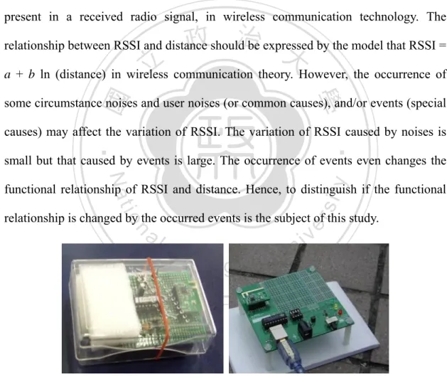
(6) LIST OF FIGURES Fig. 1.1 Transceiver (left) and receiver (right)...........................................1 Fig. 2.1 The pictures of an example experiment........................................7 Fig. 3.1 The scatter plots of Y vs. lnX for 17 experiments ...................16 Fig. 3.2 The βˆ0 chart..................................................................................20 Fig. 3.3 The βˆ1 chart..................................................................................21 Fig. 3.4 The χ Y2|ln X chart .............................................................................21. 政治大. Fig. 3.5 The monitoring results of βˆ 0 chart ...........................................22. 立. Fig. 3.6 The monitoring results of βˆ1 chart ...........................................22. ‧ 國. 學. Fig. 3.7 The monitoring results of χY2|ln X chart .....................................22. ‧. Fig. 3.8 The new βˆ0 chart........................................................................25. io. sit. y. Nat. Fig. 3.9 The new βˆ1 chart........................................................................25. er. Fig. 3.10 The new MSEY |ln X chart ...........................................................25. al. n. iv n C ˆ Fig. 3.11 The monitoring β chart .................................27 hresults e n gofcnew hi U 0. Fig. 3.12 The monitoring results of new βˆ1 chart ...................................27. Fig. 3.13 The monitoring results of new MSEY |ln X chart ........................27 Fig. 3.14 The scatter plots of X vs. t for 17 experiments.........................29 Fig. 3.15 The γˆ1 chart ..............................................................................32 Fig. 3.16 The χ X2 |t chart .............................................................................32 Fig. 3.17 The monitoring results of γˆ1 chart .........................................33 Fig. 3.18 The monitoring results of χ X2 |t chart ......................................33. III.

(7) Fig. 3.19 The confidence interval of. E (Yij | ln xi ), j = 1 ~ 3 ............................35. Fig. 3.20 The confidence interval of. E (Yij | ln xi ), j = 4 ~ 6. ..........................36. Fig. 3.21 The confidence interval of. E (Yij | ln xi ), j = 7 ~ 9. ..........................37. Fig. 3.22 The confidence interval of E (Yij | ln xi ), j = 10 ~ 12 .......................38 Fig. 3.23 The confidence interval of E (Yij | ln xi ), j = 13 ~ 15 .......................39 Fig. 3.24 The confidence interval of E (Yij | ln xi ), j = 16,17 ..........................40 Fig. 3.25 The predicted interval of Yi′*j ′ , j ′ = 18 ~ 20 ..............................42. 政治大 Fig. 3.26 The predicted 立 interval of Y , j ′ = 21 ~ 23 ..............................43 * i ′j ′. ‧ 國. 學. Fig. 3.27 The predicted interval of Yi′*j ′ , j ′ = 24 ~ 26 ..............................44. ‧. Fig. 3.28 The predicted interval of Yi′*j ′ , j ′ = 27 ~ 29 .............................45. Nat. io. sit. y. Fig. 3.29 The predicted interval of Yi′*j ′ , j ′ = 30 ~ 32 ...............................46. n. al. er. Fig. 3.30 The predicted interval of Yi ′*j ′ , j ′ = 33 ~ 35 ...............................47. Ch. engchi. IV. i Un. v.

(8) 1 INTRODUCTION The device of Babyfinder is designed to detect if an event occurs. When an event occurs, such as a child or old man gets lost, or a bicycle is stolen, the device of Babyfinder should give an alarm. In the wireless communication technology, the Babyfinder includes transceiver and receiver (see Fig. 1.1). Once there are distances between transceiver and receiver, the signal strength generates. The signal strength is called Received Signal Strength Indicator (RSSI), a measurement of the power present in a received radio signal, in wireless communication technology. The. 政治大. relationship between RSSI and distance should be expressed by the model that RSSI =. 立. a + b ln (distance) in wireless communication theory. However, the occurrence of. ‧ 國. 學. some circumstance noises and user noises (or common causes), and/or events (special causes) may affect the variation of RSSI. The variation of RSSI caused by noises is. ‧. small but that caused by events is large. The occurrence of events even changes the. y. Nat. io. sit. functional relationship of RSSI and distance. Hence, to distinguish if the functional. n. al. er. relationship is changed by the occurred events is the subject of this study.. Ch. engchi. i Un. v. Fig. 1.1 Transceiver (left) and receiver (right). A profile describes the functional relationship between the response variable and one or more explanatory variables. The goal of this study is to provide the approach of profile monitoring to ‘alarm’ changes in the functional relationship. The profile monitoring is the statistical techniques used to realize and to check the stability 1.

(9) of the functional relationship over time. The profile monitoring mainly using control charts is divided into two phases: Phase I and Phase II. In Phase I, one analyzes the historical data to model the in-control process, to evaluate stability process, and to realize the variation in the process over time. In Phase II, one uses on-line data to detect shifts in process from the baseline established in Phase I or known baseline. Many researchers have discussed profile monitoring in recent years. Woodall et al. (2004) and Woodall (2007) are relevant research papers that recommend areas for future research on profile monitoring. Most studies on profile monitoring analyze the linear profiles in Phase I and. 治政 Phase II. Kang and Albin (2000) proposed two approaches 大 to monitor simple linear 立 profiles in Phase II. First, they simultaneously monitored the profile parameters, slope ‧ 國. 學. and intercept using a multivariate T 2 control chart. Second, they used exponentially. ‧. weighted moving average ( EWMA ) chart and range ( R ) chart to monitor the mean. sit. y. Nat. and variance of the ‘residuals’ distribution, where ‘residuals’ represent the differences. io. er. between samples and the reference profile. Kim, Mahmoud, and Woodall (2003) coded the explanatory variable values to produce independent least square estimators. al. n. iv n C of the intercept and slope, so theyhcan monitor the U e n g c h i intercept and slope respectively. They used two two-sided EWMA charts to monitor the intercept and slope. separately, and a one-sided EWMA chart to monitor the error variance in Phase II. However, they recommended replacing the three EWMA charts by three Shewhart charts in Phase I because a quick detection is not the purpose in Phase I and the rule for deleting samples and for recalculating limits is not clearly defined. Mahmoud and Woodall (2004) proposed an alternative approach in Phase I through using a global. F-test to monitor the regression coefficients and a univariate control chart to monitor the variation of the regression lines. Zou et al. (2006) and Mahmoud et al. (2007) proposed a change-point monitoring method, which is especially suitable for use 2.

(10) during the set-up stages of process, for detecting the changes in parameters in Phase II and Phase I respectively. Zou et al. (2007) used a self-starting control chart based on recursive residuals to monitor linear profiles for overcoming the situation that the samples for parameter estimation are not sufficiently large. Noorossana and Amiri (2007) used a multivariate cumulative sum (MCUSUM) with the χ 2 chart to improve the performance of monitoring linear profiles in Phase II. These monitoring approaches above used fixed effects models. Shiau et al. (2006), on the other hand, monitored linear profiles with random effects.. 政治大 discussed approaches for more complicated profiles, such as non-linear profiles. 立 Except for monitoring the linear profile discussed above, many papers have. ‧ 國. 學. Walker and Wright (2002) used a general additive model, which is used to fit complicated curves in a nonparametric fashion and to assess the differences between. ‧. curves, to compare the density profiles of engineered wood boards. Ding et al. (2006). sit. y. Nat. applied some data-reduction methodology to nonlinear profiles for the high data. n. al. er. io. dimensionality resulting from the discretization of nonlinear profiles. Moguerza et al.. i Un. v. (2007) monitored fitted curves themselves rather than the parameters of model fitting. Ch. engchi. curves using support vector machines ( SVM ). Jin and Shi (2001), Reis and Saraiva (2006), Jeong, Lu and Wang (2006), Zhou, Sun and Shi (2007), and Chang and Yadama (2010) used wavelets to represent profiles or wavelet-based approaches to monitor complicated profiles. Shiau et al. (2009) also proposed approaches to monitor nonlinear profiles with random effects. To study the empirical functional relationship of RSSI (denoted as Y) and distance (denoted as X), experiments with noise factors and distance are designed. The in-control empirical model of Y and X thus determined. At the same time, the device of Babyfinder collects data of not only Y but also generated number of 3.

(11) transmitting points (denoted as t). The in-control empirical model of X and t is also investigated. However, the profile monitoring schemes trace an after-event and it has no function of real-time monitoring. A real-time monitoring scheme is proposed by considering the functional relationship of Y and t, where t is used to replace X through the empirical model of X and t, since the device cannot record the distance in reality. This study illustrates (1) how the data is collected by the design of experiments, (2) treating the collected data to 2 different dataset, (3) determining the empirical model of Y and lnX, and X and t, (4) constructing control charts to monitor the coefficients and error variance in the determined profiles, and (5) a real-time. 治政 monitoring scheme. In Chapter 2, the study describes大 how the seventeen non-stolen 立 experiments and eighteen stolen experiments are performed and processed. In Chapter ‧ 國. 學. 3, this study uses the profile monitoring scheme including using control charts to. ‧. monitor the profile of Y given the natural logical transformation of distance (denoted. sit. y. Nat. as lnX ) and to monitor the profile of X given t. The use of the prediction interval of. io. er. Y given t for real-time monitoring is considered. The performances of the using two schemes are compared. Finally in Chapter 4, a summary and conclusions are given.. n. al. Ch. engchi. 4. i Un. v.

(12) 2 DATA COLLECTION AND THE DESIGN OF EXPERIMENTS This section first describes the design of the Babyfinder experiments. To simplify, the experiments focus on the stolen bicycle problem. Before designing the experiments, we brainstormed some possible noise factors and conducted screening small experiments to identify the disturbances that significantly affect the Babyfinder device. This section adopts those significant disturbances in designing experiments. After conducting the experiments, this section presents and discusses the experiment. 政治大. data. The following subsection provides the details about these experiments.. 2.1 The Description立 of Experiments. ‧ 國. 學. The real environments have many noise factors; the experiments in this study. ‧. consider four possible kinds of noise factors: (1) interference in the vicinity of the. y. sit. io. er. vicinity of the user.. Nat. transceiver; (2) transceiver location; (3) the user's location; and (4) interference in the. From possible kinds of noise factors, we identify the significant noise factors,. al. n. iv n C which are either internal or external Table 2.1). Internal noises depend on hnoises e n g(see chi U the user, and include (1) the user’s figure (three levels: 1= thin and small, 2= normal, and 3= tall and strong), (2) user’s cell phone rings (two levels: 1= No and 2= Yes), (3) user turns around (two levels: 1= No and 2= Yes), and (4) the transceiver is in the user’s bag (two levels: 1= No and 2= Yes). External noises include (1) pedestrians passing by the user (two levels: 1= No and 2= Yes), (2) noises around the bicycle (four levels: 1= no noises, 2= a crowd of people around the bicycle, 3= someone sitting on the bicycle, and 4= a slight bicycle movement by the passenger), and (3) nearby locations (five levels: 1= a riverbank, which represents a spacious place, 2= a high building, 3= a three-story building, 4= a side door of a school, and 5= a 5.

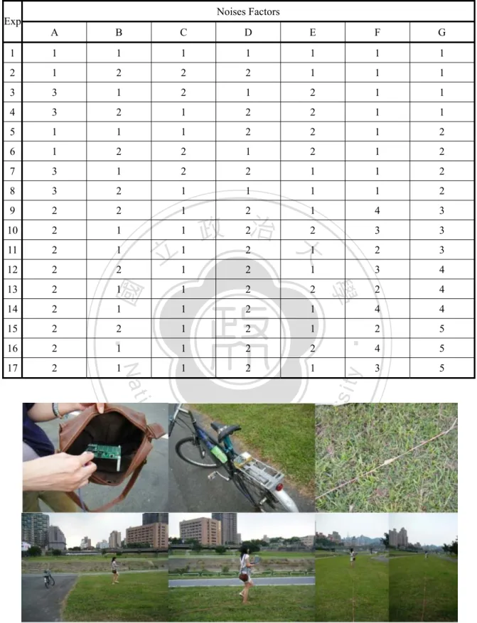
(13) schoolyard with high buildings nearby). Considering the 17 level combinations of the 7 noise factors, Table 2.2 presents the 17 experiments. Consider the following situation as an example: The user starts to walk near a riverbank. The user is thin and small, and the receiver is put in the user’s bag. Fig. 2.1 shows pictures of the example experiment. Table 2.1 The 7 internal and external noises factors Internal Noises SignLevel. Remark. Factor. 1. Thin and small. Pedestrians. 2 3. SignLevel 1. No. Normal. 2. Yes. Tall and strong 立. 1. No noises. passing by the. A crowd of people around. 1. No. the bicycle. B. Noises around Yes. al. n The transceiver is in the user’s bag. C. F. Someone sitting on the. 3. bicycle. A slight bicycle movement. er. io 1. the bicycle. sit. Nat. 2. User turns around. 2. ‧. rings. E. user 政治大. 學. User’s cell phone. A. ‧ 國. The user’s figure. Remark. y. Factor. External Noises. No. Ch. 2. Yes. 1. No. 2. Yes. engchi. i Un. v. 4. by the passenger. 1. A riverbank. 2. A high building. 3. A three-story building. 4. A side door of a school. D Nearby locations. G. A schoolyard with high 5 buildings nearby. 6.

(14) Table 2.2 The 17 non-stolen experiments Exp. Noises Factors A. B. C. D. E. F. G. 1. 1. 1. 1. 1. 1. 1. 1. 2. 1. 2. 2. 2. 1. 1. 1. 3. 3. 1. 2. 1. 2. 1. 1. 4. 3. 2. 1. 2. 2. 1. 1. 5. 1. 1. 1. 2. 2. 1. 2. 6. 1. 2. 2. 1. 2. 1. 2. 7. 3. 1. 2. 2. 1. 1. 2. 8. 3. 2. 1. 1. 1. 1. 2. 9. 2. 2. 1. 2. 1. 4. 3. 10. 2. 1. 1. 3. 3. 11. 2. 1. 2. 3. 12. 2. 2. 立 11. 13. 2. 1. 14. 2. 15. 2. 16. 2. 17. 2. 3. 4. 1. 2. 2. 2. 4. 1. 1. 2. 1. 4. 4. 2. 1. 2. 1. 2. 5. 1. 1. 2. 2. 4. 5. 1. 1. 2. 1. 3. 5. 學. 1. n. al. er. io. sit. y. ‧. Nat. 2. ‧ 國. 政 2治大2 2 1. Ch. engchi. i Un. v. Fig. 2.1 The pictures of an example experiment. 7.

(15) In this study, the data of the experiment is collected with the following steps: Step1: The distances of 3.32 m, 4.48 m, 6.05 m, 8.17 m, 11.02 m, 14.88 m, 20.09 m, 27.11 m, 36.60 m, 49.40 m, and 66.69 m are set and mark them on a rope. Step2: Place the transceiver on the bicycle and connect the receiver to a notebook computer. Step3: Choose an experiment number and set the experiment conditions. Step4: The user leaves the bicycle and walks along the rope to a predetermined distance, 66.69m. The duplicate data of the set distance is recorded. Note that the RSSI value and. 治政 t will be recorded in notebook when there is a distance 大between the transceiver and 立 receiver. ‧ 國. 學. In addition to 17 non-stolen experiments, this study also performs 18. ‧. experiments in which the bicycle was stolen at a distance 6.05 m. These experiments. sit. y. Nat. will be confirmed the validation of the proposed approach, that is, to detect out if the. io. er. bicycle has been stolen. These experiments took place at a hillside location, and considered factors such as (1) the direction of the user and bicycle (three levels: 1=. al. n. iv n C the opposite, 2= 90 degrees, and 3= (2) moving speed of bicycle (two h e45ndegrees), gchi U. levels: 1= uphill and 2= downhill), (3) method of stealing (two levels: 1= riding and 2= driving), and (4) the thief’s figure (three levels: 1= thin and small, 2= normal, and 3= tall and strong). Table 2.3 presents these factors and Table 2.4 shows the 18 stolen experiments of these factor combinations.. 8.

(16) Table 2.3 The 4 factors of possible events( bicycle is stolen at a hillside location) External Noises Factor. Sign. The direction of the user and bicycle. H. Moving speed of bicycle. I. Method of stealing. The thief’s figure. J. 立. Level. Remark. 1. The opposite. 2. 90 degrees. 3. 45 degrees. 1. Uphill. 2. Downhill. 1. Riding. 2. Driving. 政K 治 12 大. Thin and small Normal Tall and strong. 3. ‧ 國. 學. 18. 1. 1. 1. 19. 1. 1. 1. 20. 1. 2. 1. 21. 1. 2. 1. 22. 2. 23. io. n. al. K. 1. sit. J. er. I. ‧. H. Nat. Exp. y. Table 2.4 The 18 stolen experiments. n U i e h ngc 1 1. iv. 3. 3 1. 1. 2. C h2. 24. 2. 1. 1. 3. 25. 2. 2. 1. 1. 26. 2. 1. 2. 2. 27. 2. 2. 2. 2. 28. 1. 2. 2. 2. 29. 1. 1. 2. 2. 30. 3. 2. 1. 2. 31. 3. 2. 1. 2. 32. 3. 1. 1. 2. 33. 3. 1. 1. 2. 34. 3. 2. 2. 2. 35. 3. 1. 2. 2. 9. 3 1.

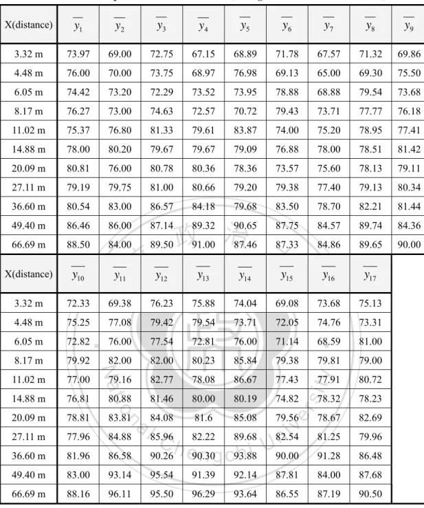
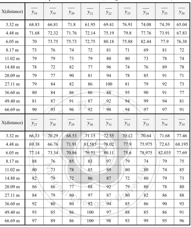
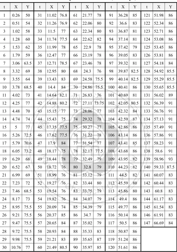
(17) 2.2 The Data Processing The collected data is treated as two datasets. One data sets with average RSSI at each set X, used to determine the empirical functional relationship of Y and lnX (called dataset1, and see Table 2.5 and Table 2.6). Another data sets with estimated X for the corresponding t (called dataset2). The details of processing dataset2 are as follows. (1) Impute X values by the distance. (2) Average the Y value at set distance X. (3) Average the previous and subsequent points of Y value missing resulted from noises to create this value. Experiment 2 provides an example, and Table 2.7 shows. 政治大. the data. This study uses dataset2 to determine the empirical functional relationship of X and t.. 立. ‧. ‧ 國. 學. n. er. io. sit. y. Nat. al. Ch. engchi. 10. i Un. v.

(18) Table 2.5 The experiment 1~17 of dataset1 (average RSSI value at set distance) X(distance). y1. y2. y3. y4. y5. y6. y7. y8. y9. 3.32 m. 73.97. 69.00. 72.75. 67.15. 68.89. 71.78. 67.57. 71.32. 69.86. 4.48 m. 76.00. 70.00. 73.75. 68.97. 76.98. 69.13. 65.00. 69.30. 75.50. 6.05 m. 74.42. 73.20. 72.29. 73.52. 73.95. 78.88. 68.88. 79.54. 73.68. 8.17 m. 76.27. 73.00. 74.63. 72.57. 70.72. 79.43. 73.71. 77.77. 76.18. 11.02 m. 75.37. 76.80. 81.33. 79.61. 83.87. 74.00. 75.20. 78.95. 77.41. 14.88 m. 78.00. 80.20. 79.67. 79.67. 79.09. 76.88. 78.00. 78.51. 81.42. 20.09 m. 80.81. 76.00. 80.78. 80.36. 78.36. 73.57. 75.60. 78.13. 79.11. 27.11 m. 79.19. 79.75. 81.00. 80.66. 79.20. 79.38. 77.40. 79.13. 80.34. 36.60 m. 80.54. 83.00. 86.57. 84.18. 79.68. 83.50. 78.70. 82.21. 81.44. 49.40 m. 86.46. 86.00. 84.57. 89.74. 84.36. 66.69 m. 88.50. 84.86. 89.65. 90.00. X(distance). y10. 89.32 90.65 87.75 治政 84.00 89.50 91.00 87.46 87.33 大立y y y y y. y16. y17. 3.32 m. 72.33. 69.38. 76.23. 75.88. 74.04. 69.08. 73.68. 75.13. 4.48 m. 75.25. 77.08. 79.42. 79.54. 73.71. 72.05. 74.76. 73.31. 6.05 m. 72.82. 76.00. 77.54. 72.81. 76.00. 71.14. 68.59. 8.17 m. 79.92. 82.00. 82.00. 80.23. 85.84. 79.38. 79.81. 79.00. 11.02 m. 77.00. 79.16. 82.77. 78.08. 86.67. 77.43. 14.88 m. 76.81. 80.88. 81.46. 80.00. 80.19. 74.82. 20.09 m. 78.81. 27.11 m. 77.96. 36.60 m. 13. 14. 15. 80.72. 78.32. 78.23. 78.67. 82.69. 81.25. 79.96. 81.96. a l 84.08 81.6 85.08 79.56i v 84.88 85.96 n C h 82.22 89.68 U82.54 i 86.58 90.26 e90.30 93.88 90.00 h ngc. 91.28. 86.48. 49.40 m. 83.00. 93.14. 95.54. 91.39. 92.14. 87.81. 84.00. 87.68. 66.69 m. 88.16. 96.11. 95.50. 96.29. 93.64. 86.55. 87.19. 90.50. er. io. sit. ‧. 77.91. Nat. 81.00. y. 12. 學. ‧ 國. 11. 87.14. n. 83.81. 11.

(19) Table 2.6 The experiment 18~35 of dataset1 (average RSSI value at set distance) X(distance). y18. y19. y20. y 21. y22. y23. y24. y25. y26. 3.32 m. 68.83. 66.81. 71.8. 61.95. 69.41. 76.91. 74.08. 74.39. 65.04. 4.48 m. 71.68. 72.32. 71.76. 72.14. 75.19. 79.8. 77.76. 73.91. 67.83. 6.05 m. 70. 73.75. 75.73. 72.75. 80.18. 75.88. 82.44. 77.9. 76.38. 8.17 m. 73. 76. 74. 72. 81. 71. 69. 81. 72. 11.02 m. 79. 79. 73. 79. 80. 80. 73. 78. 74. 14.88 m. 78. 72. 82. 77. 96. 74. 76. 89. 78. 20.09 m. 79. 77. 90. 81. 94. 78. 85. 91. 71. 27.11 m. 79. 84. 82. 86. 100. 81. 79. 92. 73. 36.60 m. 80. 84. 86. 86. 88. 95. 90. 91. 77. 49.40 m. 81. 87. 91. 99. 94. 81. 66.69 m. 90. 93. 96. 87 92 94 政92 治98 大94. 97. 97. 91. X(distance). y27. y28. y33. y34. y35. 3.32 m. 66.33. 70.29. 4.48 m. 69.38. 6.05 m. y32. 68.53. 71.15. 72.55. 70.12. 70.64. 71.68. 77.46. 66.76. 71.91. 81.585. 78.02. 77.9. 75.975. 72.63. 68.195. 77.14. 73.34. 70.86. 76.55. 80.11. 75.6. 78.975. 82.035. 77.69. 8.17 m. 88. 76. 85. 83. 97. 79. 74. 79. 75. 11.02 m. 80. 73. 78. 85. 89. 80. 80. y. 74. 85. 14.88 m. 82. 79. 72. 86. 87. 72. 80. 79. 73. 20.09 m. 86. 77. 88. 92. 79. 80. 78. 80. 27.11 m. 84. 79. 97. 87. 82. 86. 88. 36.60 m. 92. 80. Ch. 80. 85. 86. 90. 93. 49.40 m. 93. 85. 86. 100. 97. 88. 85. 86. 91. 66.69 m. 97. 89. 86. 100. 98. 93. 99. 95. 96. io. n. al. 80. e 92 n g c h94i. 12. sit. Nat 86. er. ‧ 國. y31. 29. 學. y30. ‧. 立y. v 80i n U.

(20) Table 2.7 The experiment 2 of dataset2 (for example) t. X. Y. t. 1. 0.26. 50. 31. 2. 0.51. 54. 3. 1.02. 4. X. Y. t. X. Y. t. X. Y. 11.02 76.8. 61. 21.77. 78. 91. 36.28. 85. 121 51.98. 86. 32. 11.26 76.9. 62. 22.06. 80. 92. 36.6. 83. 122 52.34. 86. 58. 33. 11.5. 63. 22.34. 80. 93. 36.87. 81. 123 52.71. 86. 1.28. 60. 34. 11.74 77.5. 64. 22.62. 82. 94. 37.14. 81. 124 53.08. 86. 5. 1.53. 62. 35. 11.99. 78. 65. 22.9. 78. 95. 37.42. 79. 125 53.45. 86. 6. 1.79. 59. 36. 12.47. 77. 66. 23.19. 78. 96. 39.05. 83. 126 53.81. 86. 7. 3.06 63.5. 37. 12.71 78.5. 67. 23.46. 78. 97. 39.32. 81. 127 54.18. 84. 8. 3.32. 69. 38. 12.95. 80. 68. 24.3. 76. 98. 39.87 82.5. 128 54.92 85.5. 9. 3.55. 64. 39. 13.43. 83. 69. 24.58 75.5. 99. 40.14 82.5. 129 55.29 85.5. 10. 3.78 68.5. 40. 14.4. 84. 70. 24.86 75.5. 100 40.41. 86. 130 55.65 85.5. 11. 4.02. 73. 41. 14.64 82.1. 81. 131 56.02. 89. 12. 4.25. 77. 42. 14.88 80.2. 80.5. 132 56.39. 91. 13. 4.48. 70. 43. 15.15. 71 26.83 76 101 40.69 治政 72 27.11 73.75 102 42.05 大. 14. 4.74. 74. 44. 15.43. 15. 5. 77. 45. 77. 立77. t. X. Y. 77. 103 42.32. 84. 133 56.76. 91. 74. 29.32. 78. 104 42.59. 87. 134 57.13. 91. 17.35 77.5. 75. 30.27. 77. 105 42.86. 86. 135 57.49. 91. 46. 17.62 77.5. 76. 31.22. 78. 106 43.14. 86. 136 57.86. 91. 47. 17.9. 84. 77. 31.54. 77. 107 43.41. 85. 91. 48. 18.17. 75. 78. 32.17 77.5. 108 43.68. 86. 138. 58.6. 91 93. 17. 5.79 70.6. 137 58.23. 18. 6.05 73.2. 19. 6.29. 68. 49. 18.44. 78. 79. 32.49. 79. 109 43.95. 82. 139 58.96. 20. 6.52. 67. 50. 18.72. 76. 80. 32.8. 79. 110 44.23. 82. 140 59.33 87.5. 21. 6.99. 69. 51. 22. 7.23. 72. 52. 23. 7.46 68.5. 53. 24. 8.17. 25. er. io. sit. 5.26 72.5. Nat. 16. y. 75. ‧. ‧ 國. 28.06. 學. 73. 82. 141 60.07. 83. 80. 142 60.44. 83. 80. 143. 60.8. 83. 54. 19.82. 76. 84. 34.07. 79. 114. 49.4. 86. 144 61.17. 83. 8.95 75.5. 55. 20.09. 74. 85. 34.39. 79. 115 49.77. 86. 145 61.54. 83. 26. 9.21 75.5. 56. 20.37. 85. 86. 34.7. 79. 116 50.14. 86. 146 61.91. 83. 27. 9.47 75.5. 57. 20.65. 84. 87. 35.02. 79. 117. 50.5. 86. 147 66.69. 84. 28. 9.72 75.5. 58. 20.93. 84. 88. 35.33. 83. 118 50.87. 86. 29. 9.98 75.5. 59. 21.21. 83. 89. 35.65. 87. 119 51.24. 86. 30. 10.76. 60. 21.49 80.5. 90. 35.97. 85. 120 51.61. 86. 77. n. a l 76 81 33.12 79 111 i44.5 v 19.27 76 45.59 n C h82 33.44 80 112 U 45.86 19.54 76 83e n 33.75 g c 79h i 113. 73. 18.99. 13.

(21) 3 DATA ANALYSIS FOR THE BABYFINDER EXPERIMENTS There are two different schemes to analyze the Babyfinder data: (1). Profile monitoring scheme. Two approaches are considered to monitor the profile. a.. Find the in-control relationship of Y and lnX, and construct the coefficients. charts and the error variance chart of the in-control model to detect the changes in the. 政治大. in-control model, under the total false alarm rate 1 − (1 − α1 ). 立. (#. of charts ). , where α1 is. the false alarm rate for one chart.. ‧ 國. 學. To construct the coefficients charts, the control limits of the coefficients charts are determined by two different methods of calibration. They are:. ‧. io. sit. y. Nat. ^ ^ ⎧ UCL = E (coefficient ) + K V (coefficient ) ⎪ , (a) Shewhart type control charts. Let ⎨ ^ ^ ⎪ LCL = E (coefficient ) − K V (coefficient ) ⎩. α1. al. n. ARL =. 1. er. where K is the width of control limits and computed for achieving in-control .. Ch. engchi. i Un. v. α ⎛ α ⎞ (b) Let UCL be the 100 × ⎜1 − 1 ⎟ percentile and LCL be the 100 × 1 2 2⎠ ⎝ percentile of all simulated coefficient obtained by bootstrap method. To construct the error variance chart, the control limits of the coefficients charts are determined by two different methods of calibration. They are: (a) Use the χ 2 distribution to determine the control limits of the error variance chart. (b) Let UCL be the 100 × (1 − α1 ) percentile of all simulated coefficient obtained by bootstrap method and let LCL be 0. 14.

(22) b.. Find the in-control relationship of X and t, and construct the coefficients charts. and the error variance chart of the in-control model to detect the changes in the in-control model under the total false alarm rate 1 − (1 − α 2 ). (#. of charts ). , where α 2 is. the false alarm rate for one chart. The approach of constructing control charts is similar to approach a. (2). Real time monitoring scheme. The profile monitoring scheme cannot detect the changes in profile in on-line production process. The real-time detection scheme is provided to improve it.. 治政 In reality, the distance X cannot be measured from 大the device but the RSSI (Y) 立 is obtained about every half second (or 400 millisecond) (t). That is, only the paired ‧ 國. 學. data (t, Y) can be obtained from the device. Hence this study may monitor the process. ‧. using the relationship of Y and t.. al. iv n C U of Y given lnX Control charts for monitoring h e n g cthe h iprofile n. 3.1.1. er. io. 3.1 The Profile Monitoring Scheme. sit. y. Nat. The following sections discuss the two different schemes.. This section attempts to identify the model of Y | lnX in the presence of noises, and uses the distribution of the estimators of the model parameters to construct the control charts, where Y represents the average RSSI value. We used dataset1 to fit the model of Y | lnX . Consider the scatter plots of 17 experiments (see Fig. 3.1). The 17 scatter plots reveal that the relationship of Y | lnX is linear.. 15.

(23) The orthogonal polynomial model is expressed as Yij ln xi = β 0 P0 (ln xi ) + β1 P1 (ln xi ) + ε Y |ln X ,ij ,. (3.1) ⎞. ⎛. where εY|ln X ,ij ~ NID(0, σY2|ln X ) , P0 (ln xi ) = 1 , and P1 (ln xi ) = 1× ⎜ ln xi − ln x ⎟ = ⎛⎜ ln xi − 2.7 ⎞⎟ , ⎟ ⎜ d. ⎝. ⎝. ⎠. 0 .3. ⎠. i = 1,2,..., n1 , j = 1,2,..., m , where d is the space of the explanatory variable,. j. denotes to be the experiment number and i denotes to be the i th observation, and there are m experiment, m=17, and each experiment is with n1 observations, n1 = 11 . The orthogonal polynomial model refers to Montgomery et al. (2001).. 政治大 ˆ. The fitted linear orthogonal polynomial model for experiment j is expressed as. 立. where βˆlj =. ∑P. l. i =1 n1. (ln xi ) yij. l. 2. , l = 0,1 , j = 1,2,..., m (see Table 3.1).. (ln xi ). ‧. ∑P i =1. (3.2). 學. n1. ‧ 國. Yîj ln x i = βˆ0 j P0 (ln xi ) + β1 j P1 (ln xi ) ,. sit. y. Nat. 2. al. n. Y1. 3. 4. 2. Y2. Y3. Ch. er. io. Scatterplot of Y j vs lnX, j=1, 2, ..., 17 3. 4. v ni Y4. engchi U. Y5 90 80 70. Y6. Y7. Y8. Y9. Y10. Y11. Y12. Y13. Y14. Y15. 90 80. Y. 70. 90 80 70 Y16. Y17. 2. 3. 4. 90 80 70 2. 3. 4. lnX. Fig. 3.1 The scatter plots of Y vs. lnX for 17 experiments. 16. 2. 3. 4.

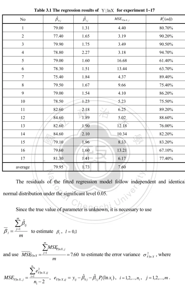
(24) Table 3.1 The regression results of Y | lnX for experiment 1~17 No. βˆ 0 j. βˆ1 j. MSEY |ln X , j. R2j (adj). 1. 79.00. 1.31. 4.40. 80.70%. 2. 77.40. 1.65. 3.19. 90.20%. 3. 79.90. 1.75. 3.49. 90.50%. 4. 78.80. 2.27. 3.18. 94.70%. 5. 79.00. 1.60. 16.68. 61.40%. 6. 78.30. 1.51. 13.44. 63.70%. 7. 75.40. 1.84. 4.37. 89.40%. 8. 79.50. 1.67. 9.66. 75.40%. 9. 79.00. 1.54. 4.10. 86.20%. 10. 78.50. 1.23. 5.23. 75.50%. 11. 82.60. 89.20%. 12. 84.60. 13. 82.60. 2.18 6.25 治政 1.89 5.02 大. 14 15 16. average. 12.18. 76.00%. 84.60. 2.10. 10.34. 82.20%. 79.10. 1.96. 8.33. 79.60. 1.60. 13.21. 81.30. 1.41. 6.17. 79.95. 1.73. 7.60. 83.20% 67.10%. ‧. 17. 1.90. 學. ‧ 國. 立. 88.60%. Nat. sit. y. 77.40%. io. al. n. normal distribution under the significant level 0.05.. Ch. engchi. er. The residuals of the fitted regression model follow independent and identical. i Un. v. Since the true value of parameter is unknown, it is necessary to use m. βl =. ∑ βˆ j =1. lj. m. to estimate β l , l = 0,1 m. and use MSEY|ln X = n1. MSEY |ln X , j =. ∑MSE j =1. ∑e i =1. 2 Y |ln X ,ij. n1 − 2. Y |ln X , j. m. = 7.60 to estimate the error variance σ Y2|ln X , where. , eY |ln X ,ij = yij − βˆ0 j − βˆ1 j P1 (ln xi ) , i = 1,2,..., n1 , j = 1,2,..., m .. 17.

(25) 17. m. Hence, β 0 =. ∑ βˆ0 j j =1. ∑ βˆ0 j j =1. =. m. 17. 17. m. = 79.95 , β 1 =. ∑ βˆ1 j j =1. m. =. ∑ βˆ j =1. 17. 1j. = 1.73 and a. synthetic regression model is ⎛ ln xi − 2.7 ⎞ Yîj ln xi = β 0 + β 1 P1 (ln xi ) = 79.95 + 1.73 × ⎜ ⎟. ⎝ 0.3 ⎠. 3.1.1.1. (3.3). Construction of Shewhart type βˆ0 , βˆ1 and χ Y2|ln X charts. It is possible to monitor the intercept, slope, and error variance of the profile of Y | lnX by monitoring the three Shewhart type charts, βˆ0 chart for monitoring. 政治大. intercept, βˆ1 chart for monitoring slope, and the χY2|ln X chart for monitoring error. 立. variance with the same probability of false alarm rate α1 = 0.0009 each such that the. ‧ 國. 學. overall in-control average run length (ARL) equals to 370 (or total false alarm rate is. ‧. 0.0027).. sit. al. iv n C U in β chart is constructedhtoemonitor h n g c thei shift. in-control, βˆ0 j ~ N ( β 0 ,. n. The βˆ0. er. The βˆ0 chart. io. a.. y. Nat. (1). The structure of βˆ0 , βˆ1 and χ Y2|ln X charts. σ Y2|ln X n1. ∑P i =1. 2 0. 0. . When the process is. ), j = 1,2,K, m . The control limits of βˆ0 chart,. (ln xi ). denoted as LCLβˆ and UCLβˆ , and the centerline, CLβˆ , are as follows. 0. 0. 0. UCL βˆ = β 0 + t α 1 0. MSE 2. , n1. n1. ∑P i =1. 2 0. Y | ln X. (ln x i ). .. CL βˆ = β 0 0. LCL βˆ = β 0 − t α 1 0. MSE 2. , n1. n1. ∑P i =1. 18. 2 0. Y | ln X. (ln x i ).

(26) b.. The βˆ1 chart The βˆ1 chart is constructed to monitor the shift in β 1 . When the process is in-control, βˆ1 j ~ N ( β1 ,. σ Y2|ln X n1. ∑P. 2 1. i =1. ), j = 1,2,K, m . The. (ln xi ). control limits of βˆ1 chart, denoted as LCLβˆ and UCLβˆ , and the centerline, CLβˆ , 1. 1. 1. are as follows. LCL βˆ = β 1 − tα1 1. MSE Y |ln X 2. , n1. ∑P 治. 政. 2 1. i =1. CL βˆ = β 1. 立. n1. 1. ‧ 國. 1. 大. MSE Y |ln X 2. , n1. n1. ∑P. 2 1. i =1. (ln xi ). 學. The χ Y2|ln X chart. ‧. c.. UCL βˆ = β 1 + tα1. (ln xi ). sit. y. Nat. To monitor the shifts in the variance of error, σ Y2|ln X the χ Y2|ln X chart is σY|ln X. n. al. statistic be χY2 ln X =. LCLχ 2. Y ln X. MSEY|ln X. and UCLχ 2. Y ln X. iv. n C h. The control limits e n g c h i U of. (n1 − 2)MSEY|ln X , j. j. er. io. Y |ln X , j considered. When the process is in-control, (n1 − 2)MSE ~ χn2 −2 , j = 1,2,K, m . Let the 2 1. χ Y2|ln X chart, denoted as. , are as follows.. UCLχ 2. = χ n21 − 2,α1. LCLχ 2. =0. Y ln X. Y ln X. ,. where the lower limit is zero since we only want to monitor the increase in variability.. 19.

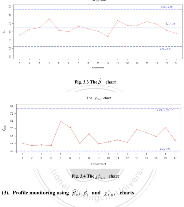
(27) (2). The Phase I βˆ0 , βˆ1 and χ Y2|ln X charts. From the in-control 17 experiments data, under α1 = 0.0009 , the control limits of the Phase I βˆ0 , βˆ1 and χ Y2|ln X charts are calculated with UCLβˆ = 83.49 , 0. CLβˆ = 79.95 , LCLβˆ = 76.41 , UCLβˆ = 2.85 , CLβˆ = 1.73 , LCLβˆ = 0.61 and 0. 0. UCLχ 2. Y ln X. 1. 1. 1. = 28.15 .. The values of βˆ0 , βˆ1 and χ Y2|ln X for the experiments are plotted in the βˆ0 ,. βˆ1 and χ Y2|ln X chart, respectively.. 立. 政治大. The βˆ 0 chart (Fig. 3.2) shows there are 3 outliers (experiment number 7, 12. ‧ 國. 學. and 14). However, they cannot be deleted since the 3 experiments are from the in. ‧. control process. Thus, they are false alarms and the chart is used to trace data. The βˆ1. sit. y. Nat. chart (Fig. 3.3) shows that there is no false alarm, so it can be used to trace data. The. io. n. al. er. χ Y2|ln X chart (Fig. 3.4) shows that there is no false alarm, so it can also be used to. i Un. v. trace data. Hence, these three charts show that experiments 7, 12 and 14 are with false alarms.. Ch. engchi. Fig. 3.2 The βˆ0 chart 20.

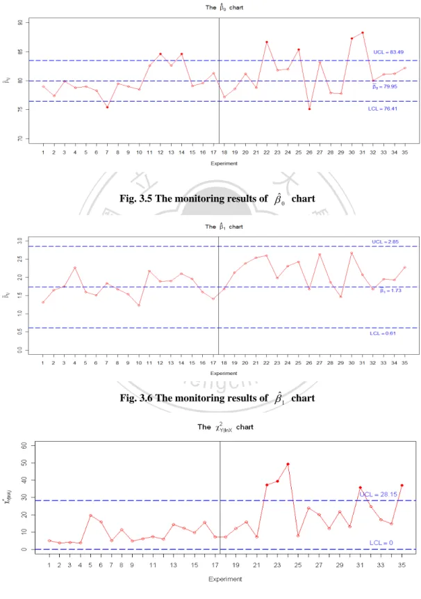
(28) Fig. 3.3 The βˆ1 chart. 政治大. 立. ‧. ‧ 國. 學 er. io. iv n ˆ ˆ C Profile monitoring using β h , β and χ e n g c h i Ucharts n. (3).. sit. y. Nat. al. Fig. 3.4 The χ Y2|ln X chart. 0. 2 Y |ln X. 1. To monitor if the profile changes on the experiment number from 18 to 35, the. βˆ0 , βˆ1 and χY2|ln X values for each experiment are computed and plotted on their chart, respectively. The βˆ0 chart (Fig. 3.5) shows that there are 12 experiments with no true alarm (experiment number 18~21, 23, 24, 28, 29 and 32~35). It means that the 12 stolen situations cannot be detected by this chart. The βˆ1 chart (Fig. 3.6) shows that all the 18 experiments are with no true alarms (experiment number 18~35). The χY2|ln X chart 21.

(29) (Fig. 3.7) shows that 13 experiments produced no true alarms (experiment number 18~21, 25~30 and 32~34). Hence, these three charts cannot detect the changes in profile for experiment number 22~27, 30, 31 and 35.. 立. 政治大. Fig. 3.5 The monitoring results of βˆ 0 chart. ‧. ‧ 國. 學. n. er. io. sit. y. Nat. al. Ch. engchi. i Un. v. Fig. 3.6 The monitoring results of βˆ1 chart. Fig. 3.7 The monitoring results of 22. χY2|ln X. chart.

(30) 3.1.1.2. Construction of βˆ0 , βˆ1 and MSEY |ln X charts using bootstrap method. The widths of control limits of the βˆ0 and βˆ1 charts depend on MSEY |ln X , j , so the βˆ0 , βˆ1 and χY2|ln X charts cannot tell the real process situation of profile. To solve the problem, that is to let the control limits of βˆ0 and βˆ1 charts independent of MSEY |ln X , the bootstrap method is proposed to determine the control limits of the. βˆ0 , βˆ1 and MSEY |ln X charts for profile monitoring.. 政治大. The procedure of bootstrap is described as follows.. 立. Step1: For experiment1, fit a linear orthogonal polynomial model (3.2) and. ‧ 國. 學. obtain the fitted values Yî1 and residuals eY |ln X ,i1 , i = 1,2,..., n1 .. Nat. sit. io. i = 1,2,..., n1 .. y. and then obtain the simulated response values. n. al. yi′1 = Yî1 + eY′ |ln X ,i1 ,. er. eY |ln X ,i1. ‧. Step2: Obtain a simulated random sample eY′ |ln X ,i1 by resampling the residuals. Ch. i Un. v. Step3: Use the simulated yi′1 and ln xi , i = 1,2,..., n1 to fit model (3.2) again,. engchi. and save the values of new βˆ0 , βˆ1 and MSEY |ln X . Step4: Repeat Step2 ~ Step3 100,000 times. Step5: Repeat Step1 ~ Step4 for experiment 2~17, so 1,700,000 values of new. βˆ0 , βˆ1 and MSEY |ln X are obtained for experiment 1~17.. 23.

(31) Step6: Rank the 1,700,000 values of new βˆ0 , βˆ1 and MSEY |ln X . Find the. 0.045 and 99.955 percentiles as the lower and upper control limits of new βˆ0 and. βˆ1 charts, respectively, to have false alarm rate α1 = 0.0009 . Find the 99.91 percentiles as the upper control limit of new MSEY |ln X chart, to have false alarm rate. α1 = 0.0009 . The lower control limit of new MSEY |ln X chart is set 0. Note that only that the residuals of the 17 experiments are homogeneous and independent this method can be used, and here they have been checked.. 政治大. The control limits of the new βˆ0 , βˆ1 and MSEY |ln X charts are UCLβˆ = 83.01 ,. 立. 0. LCLβˆ = 77.12 , UCLβˆ = 2.64 , LCLβˆ = 0.81 and UCLMSEY |ln X = 25.57 . The values of 1. ‧ 國. 1. 學. 0. βˆ0 , βˆ1 and MSEY |ln X are plotted in the new βˆ0 , βˆ1 and MSEY |ln X charts for the. ‧. experiments 1~17, respectively (see Fig. 3.8, Fig. 3.9 and Fig. 3.10).. y. Nat. er. io. sit. The new βˆ 0 chart (Fig. 3.8) shows 3 outliers (experiment 7, 12 and 14). However, they cannot be deleted since the 3 experiments are from the in control. al. n. iv n C hthe process, so they are false alarms and to trace data. The i U e nchart g cishused. βˆ1 chart (Fig.. 3.9) shows that there is no false alarm, so the chart can be used to trace data. The MSEY |ln X chart (Fig. 3.10) shows that there is no false alarm, so it can also be used to. trace data. Hence, these three charts show that experiments 7, 12 and 14 are with false alarms.. 24.

(32) Fig. 3.8 The new βˆ0 chart. 立. 政治大. ‧. ‧ 國. 學. n. engchi. er. io. Ch. βˆ1 chart. sit. y. Nat. al. Fig. 3.9 The new. i Un. Fig. 3.10 The new MSEY |ln X chart. 25. v.

(33) To monitor if the profile changes on the out-of-control experiments number from 18 to 35, the βˆ0 , βˆ1 and MSEY |ln X values for each experiment are also plotted on the new charts, respectively. The new βˆ0 chart (Fig. 3.11) shows that there are 12 experiments with no true alarm (experiment number 18~21, 23, 24, 28, 29 and 32~35). It means that the 12 stolen situations cannot be detected by this chart. The new βˆ1 chart (Fig. 3.12) shows that all the 18 experiments are with no true alarms (experiment number 18~35). The new MSEY |ln X chart (Fig. 3.13) shows that 13 experiments produced no true. 政治大 alarms (experiment number 18~21, 25~30 and 32~34). Hence, these three charts 立. ‧ 國. 學. cannot detect the changes in profile for experiment number 22~27, 30, 31 and 35. The monitoring results of the new βˆ0 , βˆ1 and MSEY |ln X charts are the same. ‧. as those of the βˆ0 , βˆ1 and χY2|ln X charts.. n. er. io. sit. y. Nat. al. Ch. engchi. 26. i Un. v.

(34) Fig. 3.11 The monitoring results of new βˆ 0 chart. 立. 政治大. ‧. ‧ 國. 學. io. sit. y. Nat. n. al. er. Fig. 3.12 The monitoring results of new βˆ1 chart. Ch. engchi. i Un. v. Fig. 3.13 The monitoring results of new MSEY |ln X chart. 27.

(35) 3.1.2. Control charts for monitoring the profile of X given t This section attempts to identify the model of X | t in the presence of noises,. and uses the distribution of estimators of the model parameters to construct the control charts. To specify the model of X | t , this study uses the dataset2 to estimate parameters of model and construct control charts. The scatter plots of the 17 in-control experiments (Fig. 3.14) reveal that the relationship of X and t is linear and with no intercept. The functional relationship of X and t is expressed as X ij ti = γ 1ti + ε X |t ,ij ,. 政治大. 立. iid. (3.4). where ε X |t ,ij ~ N (0, σ X2 t ) , i = 1,2,..., n2 , j = 1,2,..., m , where j denotes the experiment. ‧ 國. 學. number and i denotes the ith observation, and there are m experiment, m=17, and each experiment is with n2 observations, n2 = 147 . The fitted regression models is. Nat i =1 n2. ∑. x ij. i. i =1. sit. , i = 1,2,..., n2 , j = 1,2,..., m (see Table 3.2).. 2 i. t. al. (3.5). er. ∑t. γˆ1 j =. Xˆ ij = γˆ1 j t i ,. n. where. io. n2. y. ‧. expressed as. Ch. engchi. i Un. v. Since the true value of parameter is unknown, it is necessary to use m. 17. j =1. j =1. γ 1 = ∑ γˆ1 j m = ∑ γˆ1 j 17 = 0.4229 to estimate γ 1 and m. MSE X t =. ∑ MSE. X |t , j. j =1. m n. MSE X |t , j =. ∑e i =1. 2 X |t ,ij. n −1 ,. = 6.5294. to. estimate. the. error. variance. σ X2 t , where. eX |t ,ij = xij − γˆ1 j ti , i = 1,2,..., n2 , j = 1,2,..., m .. The residuals of the fitted regression model follow independent and identical normal distribution under the significant level 0.05. 28.

(36) S catterplot of Xij vs ti 0. 80. Xi1. 160. Xi2. 0 Xi3. 80. 160. Xi4. Xi5 50 25. Xi6. Xi7. Xi8. Xi9. Xi10. Xi11. Xi12. Xi13. Xi14. Xi15. 0. 50 25 0. 50 25 Xi16. Xi17. 0 0. 80. 160. 0. 80. 50 25 0 80. 160. 政治大 Fig. 3.14 The scatter plots of X vs. t for 17 experiments 立 t. 4. 7 8. 0.4230. al. 0.4240. n. 6. io. 5. 0.4240. Nat. 3. 0.4120. y. 2. 0.4260. Ch. MSE X |t , j. ‧. 1. γˆ1 j. sit. No. 學. Table 3.2 The regression result of X | t for experiment 1~17. er. 0. ‧ 國. X. 0.4280. e0.4240 ngchi. i Un. v. 6.00 4.00 6.00 5.00 7.00 7.00 7.00. 0.4250. 7.00. 9. 0.4230. 8.00. 10. 0.4270. 7.00. 11. 0.4200. 6.00. 12. 0.4240. 9.00. 13. 0.4220. 7.00. 14. 0.4210. 6.00. 15. 0.4210. 6.00. 16. 0.4220. 6.00. 17. 0.4230. 7.00. Average. 0.4229. 6.5294. 29. 160.

(37) Hence, a synthetic regression model is Xˆ ij = γ 1ti = 0.4229ti .. (3.6). Since the detection results of the two different methods of control limits calibration in section 3.1.1 are the same and all poor, this subsection just illustrates the first method in constructing charts. 3.1.2.1. Construction of Shewhart type γˆ1 and χ X2 |t charts. It is possible to monitor γ 1 and σ X2 t by constructing the γˆ1 chart and. 政治大. the χ X2 |t chart with the same probability of false alarm rate α 2 = 0.00135 each such. 立. that the overall in-control ARL equals to 370.. ‧ 國. 學. (1). The structure of γˆ1 and χ X2 |t charts. The γˆ1 chart. Nat. sit. The γˆ1 chart is constructed to monitor the shift in γ 1 .. y. ‧. a.. ∑ tn i v. n. al. 2. Ch. er. io. 2 When the process is in-control, γˆ ~ N (γ , σ X t ) , j = 1,2,..., m . The control 1j 1 n. engchi U i =1. 2 i. limits of γˆ1 chart, denoted as LCLγˆ1 and UCLγˆ1 , and the centerline, CLγˆ1 , are as follows. UCL γˆ1 = γ 1 + Z α 2 × 2. MSE X |t n2. ∑t i =1. 2 i. CL γˆ1 = γ 1 LCL γˆ1 = γ 1 − Z α 2 × 2. MSE X |t n2. ∑t i =1. 30. 2 i.

(38) b.. The χ X2 |t chart To monitor the shifts in the variance of error, σ X2 t the χ X2 |t chart is considered.. When the process is in-control,. Let the statistic be χ X2 t =. (n2 − 1)MSEX |t , j. σ. 2 Xt. (n2 − 1)MSEX |t , j. j. ~ χ n22 −1 , j = 1,2,..., m .. .. MSE X t. The control limits of χ X2 |t chart, denoted as LCLχ 2 and UCLχ 2 , are as follows. X t. UCLχ 2 = χ n22 −1,α 2 X t. LCLχ 2 = 0. X t. ,. 政治大 where the lower limit is zero for since we only want to monitor the increase in 立 X t. ‧ 國. 學. variability.. (2). The Phase I γˆ1 and χ X2 |t charts. ‧. y. n. al. CLγˆ1 = 0.4229. UCLχ 2 = 202.6223 X t. The value of. Ch. i Un. from the data of 17 experiments.. engchi. ,. sit. UCLγˆ1 = 0.4308 ,. er. with. io. calculated. Nat. Under α 2 = 0.00135 , the control limits of the γˆ1 and χ X2 |t chart are LCLγˆ1 = 0.4150. and. v. γˆ1 and χ X2 |t for 17 experiments are plotted in the γˆ1 and χ X2 |t. chart, respectively. The γˆ1 chart (Fig. 3.15) shows that the experiment 2 is an outlier. However, it cannot be deleted since the experiment is from in control process, so it is a false alarm. The. γˆ1 chart is thus used to trace data. The χ X2 |t chart (Fig. 3.16) shows no false. alarm, so it can be used to trace data. Hence, the two charts show that only experiment 2 is a false alarm.. 31.

(39) Fig. 3.15 The γˆ1 chart. 立. 政治大. ‧. ‧ 國. 學. n. al. Ch. engchi. er. io. 2. sit. y. Nat Fig. 3.16 The χ X |t chart. i Un. v. (3). Profile monitoring using γˆ1 and χ X2 |t charts. To monitor if the profile changes on the experiment number from 18 to 35, the. γˆ1 and χ X2 |t value for each experiment are computed and plotted on their chart, respectively. The γˆ1 chart (Fig. 3.17) shows that all the experiments with true alarm. The. χ X2 |t chart (Fig. 3.18) shows that experiment number 18 produced no true alarms. Therefore, the two charts can detect the changes in profile for all 18 experiments. That is, the performance of the two charts is very good. 32.

(40) Fig. 3.17 The monitoring results of γˆ1 chart. 立. 政治大. ‧. ‧ 國. 學. n. hengchi. chart. er. io. a. l C Scheme 3.2 Real Time Monitoring. χ X2 |t. sit. y. Nat. Fig. 3.18 The monitoring results of. i Un. v. The profile monitoring scheme is an after-event tracing approach. It seems late to detect the changes in profile. To have the function of real-time detection for the device, this section provides a real-time monitoring scheme to monitor the RSSI of the Babyfinder. Using the paired data of (t, Y), Y may be monitored by real time t. First, use the fitted 17 regression models to estimate a synthetic regression model, that is ⎛ ln xi − 2.7 ⎞ Yîj ln xi = β 0 + β 1 P1 (ln xi ) = 79.95 + 1.73 × ⎜ ⎟ (see (3.3)). Secondly, estimate ⎝ 0.3 ⎠. the confidence interval of the synthetic regression model as Phase I chart. Third, 33.

(41) construct the predicted interval of a new observation ( Y * ) to trace if the process is out-of-control. The 99.73% confidence interval (CI) of the synthetic regression model is as follows: CI ⎛ ⎡ ⎜ ⎢1 ⎜ˆ MSE Y |ln X ⎢ + = ⎜ Yij − t⎛ α ⎞ ⎜ , n1 − 2 ⎟ ⎢ n1 ⎝2 ⎠ ⎜ ⎢ ⎜ ⎣ ⎝. ⎡ ⎤ ⎢1 ln xi − ln x ⎥ ˆ ⎥ ,Yij + t⎛ α MSE Y |ln X ⎢ + n1 ⎞ 2⎥ ⎜ , n1 − 2 ⎟ ⎢ n1 ⎝2 ⎠ ln xk − ln x ⎥ ∑ ⎢ k =1 ⎣ ⎦. (. ). 2. (. (. ). ). ⎤ ⎞⎟ ln xi − ln x ⎥ ⎟ ⎥⎟ n1 2⎥ ln xk − ln x ⎥ ⎟ . ∑ k =1 ⎦ ⎟⎠. (. ). 2. (. (. ). (3.7). ). 2 2 ⎞ ⎛ ⎡1 ⎡1 ln xi − 2.7 ⎤ ˆ ln xi − 2.7 ⎤ ⎟ ⎜ = ⎜ Yîj − t⎛ 0.0027 × + + × + 7.60 , 7.60 Y t ⎢ ⎥ ⎢ ⎥⎟ ij 0 . 0027 ⎞ ⎛ ⎞ ,11 − 2 ⎟ ,11− 2 ⎟ ⎜ ⎜ 9.9 9.9 ⎜ ⎢⎣11 ⎥⎦ ⎢⎣11 ⎥⎦ ⎟ ⎝ 2 ⎠ ⎝ 2 ⎠ ⎝ ⎠ 2 2 ⎞ ⎛ ⎡1 ⎡1 ln xi − 2.7 ⎤ ˆ ln xi − 2.7 ⎤ ⎟ ⎜ = ⎜ Yîj − 4.0942 × 7.60 × ⎢ + ⎥ ,Yij + 4.0942 × 7.60 × ⎢ + ⎥⎟ 9.9 9.9 ⎜ ⎣⎢11 ⎦⎥ ⎣⎢11 ⎦⎥ ⎟⎠ ⎝. (. ). 立. 政治大(. ). ‧ 國. 學. The 17 experimental paired data of (ln xi , yij ) , i = 1,2,K ,11, j = 1,2,K ,17 , are plotted in the CI to check if the 17 paired data are from the in control experimental. ‧. situations (see Fig. 3.19, Fig. 3.20, Fig. 3.21, Fig. 3.22, Fig. 3.23 and Fig. 3.24). Fig.. y. Nat. sit. 3.19~Fig. 3.24 show that there are 7 experiments with alarms (experiments 2, 5~7,. n. al. er. io. 12, 14 and 15). These alarms are investigated if they are influenced by special case,. i Un. v. since no any special case occurs, the alarms are false alarms.. Ch. engchi. 34.

(42) 立. 政治大. ‧. ‧ 國. 學. n. er. io. sit. y. Nat. al. Ch. engchi. i Un. v. Fig. 3.19 The confidence interval of E (Yij | ln xi ), j = 1 ~ 3 35.




(46) 立. 政治大. ‧. ‧ 國. 學. n. er. io. sit. y. Nat. al. Ch. engchi. i Un. v. Fig. 3.23 The confidence interval of E (Yij | ln xi ), j = 13 ~ 15. 39.

(47) 政治大. 立. ‧. ‧ 國. 學. n. er. io. sit. y. Nat. al. Ch. engchi. i Un. v. Fig. 3.24 The confidence interval of E (Yij | ln xi ), j = 16,17. The predicted interval (PI) with confidence coefficient 0.9973 of a new observation is determined as (3.8). PI ⎛ ⎤ ⎞⎟ ⎡ ⎤ ⎡ ⎜ 2 ⎥ 2 ⎥ * * ⎢ ⎢ ⎟ ⎜ 1 ln x − ln x 1 ln x − ln x ⎥⎟ ⎥ ,Yî *′j ′ + tα MSEY |ln X ⎢1 + + n1 i ′ MSEY |ln X ⎢1 + + n1 i ′ = ⎜ Yî *′j ′ − tα , n1 − 2 , n1 − 2 2⎥ 2⎥ n n ⎢ ⎢ 1 1 2 2 ⎜ ln xk − ln x ⎥ ⎟ . ln xk − ln x ⎥ ∑ ∑ ⎢ ⎢ ⎜ k =1 k =1 ⎦ ⎟⎠ ⎣ ⎦ ⎣ ⎝ ⎛ ⎡ 1 ln x*′ − 2.7 2 ⎤ ⎞⎟ ⎡ 1 ln xi*′ − 2.7 2 ⎤ * ⎜ i = ⎜ Yî *′j ′ − 4.0942 × 7.60 × ⎢1 + + ⎥⎟ ⎥ ,Yî ′j ′ + 4.0942 × 7.60 × ⎢1 + + 11 9.9 11 9.9 ⎜ ⎢ ⎥⎦ ⎟⎠ ⎢ ⎥ ⎣ ⎣ ⎦ ⎝. (. (. ). (. (. ). ). (. 40. ). (. ). ). (3.8).

(48) To monitor the future process, the new paired ( ti*′ , Yi′*j′ ) should be plotted in the constructed PI. However, the PI in (3.8) is in terms of ln xi*′ (a new observation xi*′ ). To express the PI in terms of ti*′ , the xi*′ in the PI is replaced by xî′j ′ = 0.4229ti*′ since the relationship of X and t is Xˆ = 0.4229t (see (3.9)). PI. ( (. ). ). ( (. ). ). ⎛ ⎡ 1 ln 0.4229t *′ − 2.7 2 ⎤ * ⎡ 1 ln 0.4229t *′ − 2.7 2 ⎤ ⎞⎟ ⎜ i i = ⎜ Yî′*j′ − 4.0942 7.60× ⎢1 + + ⎥ ,Yî′j′ + 4.0942 7.60× ⎢1 + + ⎥⎟ 11 9.9 11 9.9 ⎜ ⎢ ⎥ ⎢ ⎣ ⎦ ⎣ ⎦⎥ ⎟⎠ ⎝. (3.9) .. Plot the new points ( ti*′ , Yi′*j′ ), i′ = 1,2 ,K , j ′ = 18,19 ,K ,35 , of experiments 18~35. 治政 of Dataset2 into the predicted interval (see Fig. 3.25,大 Fig. 3.26, Fig. 3.27, Fig. 3.28, 立 Fig. 3.29 and Fig. 3.30, where the vertical line represents the time point of stealing). ‧ 國. 學. Fig. 3.25~Fig. 3.30 further show that there are 16 experiments with no true alarms. ‧. (experiments 18~23, 25~28 and 30~35). The performance is bad since there are 16. n. al. er. io. sit. y. Nat. out of 18 experiments cannot be detected.. Ch. engchi. 41. i Un. v.

(49) 立. 政治大. ‧. ‧ 國. 學. n. er. io. sit. y. Nat. al. Ch. engchi. i Un. v. Fig. 3.25 The predicted interval of Yi ′*j ′ , j ′ = 18 ~ 20. 42.

(50) 立. 政治大. ‧. ‧ 國. 學. n. er. io. sit. y. Nat. al. Ch. engchi. i Un. v. Fig. 3.26 The predicted interval of Yi ′*j ′ , j ′ = 21 ~ 23 43.





(55) 3.3 Performance Comparisons of the Profile Monitoring and Real Time Monitoring Schemes This study summarizes the two schemes in Table 3.3 and Table 3.4. The false alarms of the two schemes for the in-control experiments are summarized in Table 3.3 , this study can find that: 1.. For the approach of monitoring profile of Y | lnX , the results of the Shewhart type control limits and the control limits by bootstrap are the same.. 2.. For profile monitoring schemes, the approach of monitoring profile of X | t. 政治大 and real time monitoring. is better than that of Y | lnX since fewer experiments with false alarms. 3.. 立. Compare the profile. schemes, real time. ‧. ‧ 國. has.. 學. monitoring scheme has more false alarms than profile monitoring scheme. Therefore, the performance using the approach of monitoring the profile of X | t. Nat. sit. y. is the best because it is only with 1 false alarm.. n. al. er. io. The detect performance of the two schemes for the out-of-control experiments are summarized in Table 3.4. 1.. Ch. engchi. i Un. v. For the approach of monitoring profile of Y | lnX , the results of the Shewhart type control limits and the control limits by bootstrap are the same.. 2.. For profile monitoring schemes, monitoring profile of X | t is better than that of Y | lnX since all experiments with true alarms.. 3.. Compare the profile scheme and real time monitoring scheme, profile monitoring scheme has more true alarms than real time monitoring scheme has.. The performance using the approach of monitoring the profile of X | t is the best because it is with all true alarms. 48.

(56) Scheme Exp β0. ○. ○. ○. ○. ○. ○. ○. ○. ○. ○. 0. 0. 政 ○治大 ○. ○ ○ ○. 3. 3. 0. 0. 3. 1. 0. 1. 8 8. 8 8. 8 8 8 8 12. 8 8 8 8 8 8 8 8 8 8 8 8 8 8 8 8 8 8 18. 8 8 8 8. 8 8 8 8. y. sit. 8 8 8. 8 8 8 8 8 8 8 8. 8 8. 8 8 8. 8 8 8. 13. 9. 8 8. 8 8 8 8 12. er. a8l. n. 8 8 8 8. io. β0. 18 19 20 21 22 23 24 25 26 27 28 29 30 31 32 33 34 35 Total. Table 3.4 No true alarms in the out-of-control experiments Profile Monitoring Scheme Real Time Monitoring profile of X | t Monitoring Scheme Monitoring profile of Y | lnX Dataset1 Dataset2 Dataset 1 and 2 Shewhart Bootstrap χ X2 |t β1 χY2|ln X Total β 0 β1 MSEY |ln X Total Total PI r1. Nat. Exp. 7. ‧. Note: ○ indicates false alarm.. Scheme. ○. ○ ○ ○. ○. 立. ‧ 國. 3. ○. 學. 1 2 3 4 5 6 7 8 9 10 11 12 13 14 15 16 17 Total. Table 3.3 False alarms in the in-control experiments Profile Monitoring Scheme Real Time Monitoring profile of X | t Monitoring Scheme Monitoring profile of Y | lnX Dataset1 Dataset2 Dataset 1 and 2 Shewhart Bootstrap χ X2 |t β1 χY2|ln X Total β 0 β1 MSEY |ln X Total Total CI r1. 8 8 8 n8i C 8h8 8 U e8 n g8 c h i 8 8 8 8 8 8 8 8 8 8 8 8 8 8 8 8 18. 8. 8 8 8 8 8 8. v. 8 8 8 8 8 8. 8. 8 8 8 8. 8 8. 8 8 8. 8 8 8. 13. 9. Note: 8 indicates no the true alarm.. 49. 0. 1. 0. 8 8 8 8 8 8 16.

(57) These results show that the performance of monitoring profiles of X | t is best one approach among proposed schemes, producing only one false alarm and detecting all out-of-control experiments. However, a prerequisite to this method is that the device can measure X. This study recommends that the device of Babyfinder can be added the function of recoding the distance between the transceiver and receiver. Therefore, the monitoring approach for profile of X | t might be more suitable for this case.. 立. 政治大. ‧. ‧ 國. 學. n. er. io. sit. y. Nat. al. Ch. engchi. 50. i Un. v.

(58) 4 SUMMARY AND CONCLUSIONS This study attempts to find a better approach to distinguish between events and noises for the device of Babyfinder. The seventeen non-stolen experiments are designed to collect data and determine the in-control profile. To measure the performance of the proposed approached, the eighteen experiments are designed. This study proposes two schemes to control and monitor the 35 experiment data of Babyfinder. One is the profile monitoring scheme, which studies the empirical functional relationship of Y and X and that of X and t. The study uses the coefficients. 政治大 . The other is a real-time monitoring scheme that. and error variance control charts to monitor the parameters of the profiles of Y | lnX. 立. and that of the profiles of X | t. ‧ 國. 學. monitors Y by a real-time t. It is used to solve the problem that the device cannot measure the distance and to overcome the shortcut of the profile scheme.. ‧. From the detection ability of the proposed control charts, the charts in the. sit. y. Nat. approach of monitoring the profile of X and t detect all changes in profiles and only. n. al. er. io. has one false alarm; that is, their detection ability is the best. The profile monitoring. i Un. v. approach of X and t is thus recommended. However, in real situation, the distance(X). Ch. engchi. cannot be measured by the device. It is suggested to add the function of distance measuring in the device. The performance of the proposed real time monitoring approach using the prediction interval of Y | t is also not good. One of the possible reasons might be that the replacement of X value by t causes the uncertainty. Hence, an approach of a simultaneous confidence band might be a better way to solve the problem. Besides, the study of some other potential real-time detection approaches is a worthy research topic in the future.. 51.

(59) REFERENCES [1] Chang, S. I. and Yadama, S. (2010). Statistical Process Control for Monitoring Nonlinear Profiles Using Wavelet Filtering and B-Spline Approximation. International Journal of Production Research, 48(4), 1049-1068. [2] Ding, Y., Zeng, L. and Zhou, S. (2006). Phase I Analysis for Monitoring Nonlinear Profile Signals in Manufacturing Processes. Journal of Quality Technology, 38 (3), 199-216. [3] Jeong, M. K, Lu, J. C. and Wang, N. (2006). Wavelet-based SPC Procedure for Complicated Functional Data. International Journal of Production Research, 44 (4), 729-744.. 政治大. [4] Jin, J. and Shi, J. (2001). Automatic Feature Extraction of Waveform Signals of In-process Diagnostic Performance Improvement. Journal of Intelligent Manufacturing, 12 (3), 257-268.. 立. ‧ 國. 學. ‧. [5] Kang, L. and Albin, S. L. (2000). On-Line Monitoring When the Process Yields a Linear Profile. Journal of Quality Technology, 32, 418-426.. sit. y. Nat. [6] Kim, K., Mahmoud, M. A. and Woodall, W. H. (2003). On the Monitoring of Linear Profiles. Journal of Quality Technology, 35(3), 317-328.. er. io. [7] Mahmoud, M. A. and Woodall, W. H. (2004). Phase I Analysis of Linear Profiles with Calibration Applications. Technometrics, 46(4), 380-391.. al. n. iv n C h e nI gAnalysis (2008). Phase of Multiple chi U. [8] Mahmoud, M. A. Linear Regression Profiles. Communications in Statistics—Simulation and Computation, 37(10), 2106-2130. [9] Mahmoud, M. A., Parker, P. A., Woodall, W. H. and Hawkins, D. M. (2007). A Change Point Method for Linear Profile Data. Quality and Reliability Engineering International, 23(2), 247-268. [10] Mahmoud, M. A., Morgan, J. P. and Woodall, W. H. (2009). The Monitoring of Simple Linear Regression Profiles with Two Observations per Sample. Journal of Applied Statistics, (Manuscript ID: CJAS-2009-0012.R1). [11] Moguerza, J. M., Munoz, A. and Psarakis, S. (2007). Monitoring Nonlinear Profiles using Support Vector Machines. Lecture Notes in Computer Science, 4756, 574-583. 52.

(60) [12] Montgomery, D. C., Peck, E. A. and Vining, G. G. (2001). Introduction to Linear Regression Analysis. (3rd Ed.). New York: Wiley. [13] Noorossana, R. and Amiri, A. (2007). Enhancement of Linear Profiles Monitoring in Phase II. AmirKabir Journal of Science and Technology, 18, 19-27 in Farsi [14] Reis, M. S. and Saraiva, P. M., (2006). Multiscale Statistical Process Control of Paper Surface Profiles. Quality Technology and Quantitative Management, 3 (3), 263-282. [15] Shiau, J. J. H., Huang, H. L., Lin, S. H. and Tsai, M. Y. (2009). Monitoring Nonlinear Profiles with Random Effects by Nonparametric Regression. Communications in Statistics - Theory and Methods, 38(10), 1664-1679.. 政治大. [16] Shiau, J. J. H., Lin, S. H. and Chen, Y. C. (2006). Monitoring Linear Profiles Based on a Random-effect Model. Technical Report. Institute of Statistics, National Chiao Tung University, Hsinchu, Taiwan.. 立. ‧ 國. 學. [17] Walker, E. and Wright, S. (2002). Comparing Curves Using Additive Models. Journal of Quality Technology, 34 (1), 118-129.. ‧. io. sit. y. Nat. [18] Woodall, W. H, Spitzner, D. J., Montgomery, D. C. and Gupta, S. (2004). Using Control Charts to Monitor Process and Product Quality Profiles. Journal of Quality Technology, 36(3), 309-320.. n. al. er. [19] Woodall, W. H. (2007). Current Research on Profile Monitoring. Revista Producao, 17(3), 420-425.. Ch. engchi. i Un. v. [20] Zhou, S. Y., Sun, B. C. and Shi, J. J. (2007). An SPC Monitoring System for Cycle-based Waveform Signals using Haar Transform. IEEE Transactions on Automation Science and Engineering, 3(1), 60-72. [21] Zou, C., Tsung, F. and Wang, Z. (2007). Monitoring General Linear Profiles using Multivariate Exponentially Weighted Moving Average Schemes. Technometrics, 49(4), 395-408. [22] Zou, C., Zhang, Y. and Wang, Z. (2006). Control Chart Based on Change-point Model for Monitoring Linear Profiles. IIE Transactions. 38(12), 1093-1103. [23] Zou, C., Zhou, C., Wang, Z. and Tsung, F. (2007). A Self-Starting Control Chart for Linear Profiles Journal of Quality Technology, 39(4), 364-375.. 53.

(61)