Stochastic Trigonometry and Stochastic Invariants
Ovidiu Calin1 Der-Chen Chang2Abstract: We study a geometry where each point is described by stochastic coordinates. In the first part we deal with a stochastic analog of trigonometry and provide some applications in the stochastic framework. In the second part we introduce the concept of stochastic transforms which are transforms which commute with the expectation operator and study their properties. In the last part we prove that these transforms are harmonic and discuss the geometry induced by them.
Key words: normal distribution, stochastic invariant, harmonic function, Brownian motion MS Classification (2000): Primary: 51K99, 60J65 ; Secondary: 60E05
Introduction
When measuring a length for instance, one introduces inadvertently some errors of measure-ment. Since these errors are due to multiple independent causes, by the central limit theorem it makes sense to consider these errors normally distributed with zero mean. For instance if a square has the side equal to `, and the error of measurement is denoted by ², with ² ∼ N (0, k) (normally distributed with zero mean and standard deviation k), then the measured length is a random variable equal to ˆ` = ` + ². Then the estimated area of the square computed from
the measured length is given by
E(ˆ`2) = E¡(` + ²)2¢= `2+ E(²2) = `2+ k2,
which is with an amount k2larger than the real area of the square. This might be a significant
error, especially if the errors tend to cumulate as new measurements are made. If one continues with estimating the volume of a cube of side `, then we obtain
E(ˆ`3) = `3+ 3`k2+ O(²3),
which implies an error which cannot be neglected since increases linearly with respect to the cube side `.
It is important in our analysis to distinguish between the properties of the elements we are measuring. Some of them are stochastic elements, which means that one or more underly-ing parameters are random variables, and the other are fixed elements that are deterministic elements which can be measured exactly. We shall discuss next the case of a few stochastic elements such as points, lines, and circles.
A stochastic point ˆM in the plane is a point with at least one of the coordinates stochastic.
(The hat will always be used to denote a stochastic element). If ( ˆXM, ˆYM) are the Cartesian coordinates of ˆM , then either ˆXM, or ˆYM or both coordinates are random variables. The
1Partially supported by the NSF Grant #0631541
2Partially supported by the Hong-Kong RGC grant #600607 and a competitive research grant at Georgetown
expected position of the stochastic point ˆM is E( ˆM ) =¡E( ˆXM), E( ˆYM)¢= (XM, YM) = M .
A fixed point M is a point with both coordinates (XM, YM) deterministic.
For instance, due to vibration, a molecule contained in a piece of paper does not have fixed coordinates; its coordinates are stochastic, so that one can think of it as a stochastic point in the plane. If three such molecules are considered, the area of the triangle defined by them is a random variable. One problem is whether one can recover the expected area of this triangle from the expected positions of the molecules. If the answer is positive we say that we have obtained a stochastic invariant; in general this concept stands for some measurable concept which is not lost in the stochasticity and can be recovered. The same mechanism can be applied for the center of mass of the molecules, for instance. More stochastic invariants will be investigated in section 3. These stochastic invariants will be used to define the stochastic transforms of the plane in the section 4.
A stochastic line in the standard form y = ˆmx + ˆb has at least one of the parameters ˆm
or ˆb stochastic. If only the slope is stochastic, then the sample space consists of lines passing through the fixed point (0, b). If just the parameter ˆb is stochastic, then the sample space consists of a family of parallel lines of slope m.
A stochastic circle C( ˆO, ˆr) might have either a stochastic radius ˆr or a stochastic center
ˆ
O, or both. One may define any type of stochastic polygon if at least one of the vertices is a
stochastic point.
In the first part of this paper we introduce a new type of trigonometry with stochastic elements. Here we shall discuss the stochastic sine and stochastic cosine functions and their properties. A few applications given in section 2 will show how different the new geometry with stochastic elements can be from the Euclidean one.
In section 3 we shall investigate those properties which are stochastically invariant. This leads to the definition of the stochastic invariants. We provide examples of stochastic invariants on the stochastic line (the line where the coordinate is stochastic) and on the stochastic plane (the plane where the cartesian coordinates are stochastic).
In section 4 we introduce the concept of stochastic transform and study its properties. In section 5 we provide the theorems of characterization of stochastic transforms on the stochastic line and stochastic plane as linear and harmonic functions, respectively. In the fifth section we deal with the geometry introduced by the invertible stochastic transforms and discuss its rela-tionship with the metrical and affine geometries. In the last section we assume the coordinates of the point depend on time and are defined as Brownian motions and show that their images through a stochastic transform are also Brownian motions with a different time scale.
Both authors would like to thank the National Center for Theoretical Sciences in Taiwan for warm hospitality and for partial support of this research. Part of the research work was completed during the second author visits to Taiwan during the winter of 2009. The second author take great pleasure in expressing his thanks to Professor Winnie Li, the director of NCTS, for the invitation.
1
Stochastic trigonometric functions
This section defines two stochastic functions, called stochastic sine and stochastic cosine, which play a similar role to the functions sine and cosine from the usual trigonometry.
Consider a fixed point M on the fixed trigonometric circle C(O, 1). Let t be its argument, so the fixed coordinates of M are XM = cos t and YM = sin t. Now we shall consider that
due to some measurement error the angle t becomes stochastic and is replaced by the random variable τt= ˆt = t + ²t, where the error ²t∼ N (0, kt). The standard deviation ktis considered
smooth with respect to the parameter t. The probability density function of ²twill be denoted
by ϕt.
The corresponding stochastic point ˆM will have the stochastic coordinates ˆXM = cos τtand
ˆ
YM = sin τt. The expected position of the stochastic point ˆXM is E( ˆM ) = M = (XM, YM).
In order to find the expected coordinates XM, YM we shall compute the terms E(sin ²t) and
E(cos ²t) first. We have
E(sin ²t) = Z R sin x ϕt(x) dx = Z R sin x√1 2πkt e− x2 2k2t dx = 0,
as the integral of an odd function over a symmetric interval. Since
E(cos ²t) =
Z
cos x ϕt(x) dx, (1.1)
the density function ϕt(x) determines uniquely the value of E(cos ²t). Then it will suffice to
compute E(cos ²t) in the case of a particular random variable with the same density function as ²t. Choosing this random variable to be √kt
tWt, t > 0, where Wtis the 1-dimensional Brownian
motion, we note that
kt √ tWt∼ N (0, kt). Then E(cos ²t) = E¡cos(√kt tWt) ¢ = E¡cos(σtWt)¢, (1.2)
with σt=√ktt. Using that (see [2], p. 56)
E(Wt2n+1) = 0, E(Wt2n) =
(2n)! 2nn!t
n, (1.3)
taking the expectation operator in the series expansion yields
E¡cos(σtWt)¢ = X(−1)n 1 (2n)!σ 2n t E(Wt2n) = X (−1)n 1 (2n)!σ 2n t (2n)! 2nn!t n = X(−1)n 1 n! ³ σ2 tt 2 ´n = e−σ2 tt/2.
Substituting in (1.2) we get
E(cos ²t) = e−k2t/2. (1.4)
Then the value of the expected coordinates XM and YM are
XM = E( ˆXM) = E(cos τt) = E
¡
cos(t + ²t)
¢
= E(cos t cos ²t− sin t sin ²t)
= cos t E(cos ²t) − sin t E(sin ²t) = cos t E(cos ²t)
= e−k2 t/2cos t. YM = E( ˆYM) = E(sin τt) = E ¡ sin(t + ²t) ¢
= E¡sin t cos ²t+ cos t sin ²t
¢ = sin t E(cos ²t) + cos t E(sin ²t)
= e−kt2/2sin t.
Proposition 1.1 The expected coordinates of the stochastic point ˆM (cos ²t, sin ²t) are given by
(e−k2
t/2cos t, e−k2t/2sin t).
The distance between the origin and the expected position of the stochastic point ˆM is
|OM | = e−k2
t/2 ≤ 1. The trade-off between the radius length and the angle accuracy can be
stated by saying the larger the error, the shorter the radius. Since the largest error in measuring the argument angle t is π (an error of π + δ counts as δ), the shrinking factor has the lower and upper bounds
1 ≥ e−k2
t/2≥ e−π2/2.
In the next definition we shall consider the standard deviation kt= k, constant.
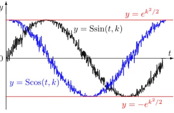
Definition 1.2 Let t be an angle measured within the error ² ∼ N (0, k), k > 0 constant. Define the stochastic functions
Ssin(t, k) = ek2/2sin(t + ²) Scos(t, k) = ek2/2cos(t + ²),
called stochastic sine and stochastic cosine of parameter k.
By Proposition 1.1 we have E¡Ssin(t, k)¢ = sin t E¡Scos(t, k)¢ = cos t, We also have Ssin2(t, k) + Scos2(t, k) = ek2 > 1.
We notice the asymptotic relations for k → 0
Ssin(t, k) → sin t, Scos(t, k) → cos t. Since if ² ∼ N (0, k) then also −² ∼ N (0, k), we have
Scos(−t, k) = ek2/2
cos(−t + ²) = ek2/2
cos(t − ²) = Scos(t, k),
i.e. t → Scos(t, k) is an even function. Similarly we can show that t → Ssin(t, k) is an odd function.
Next we shall deal with some trigonometric formulas for the stochastic sine and cosine.
Proposition 1.3
Ssin(t + u, k) = Scos(u, k) sin t + Ssin(u, k) cos t = Scos(t, k) sin u + Ssin(t, k) cos u,
Scos(t + u, k) = cos t Scos(u, k) − sin t Ssin(u, k) = cos u Scos(t, k) − sin u Ssin(t, k).
Proof: Stating from the definition we have
Ssin(t + u, k) = ek2/2
sin(t + u + ²) = ek2/2
sin¡t + (u + ²)¢
= ek2/2¡
sin t cos(u + ²) + cos t sin(u + ²)¢ = sin t Scos(u, k) + cos t Ssin(u, k). In a similar way we can prove the other formulas.
The graphs of the stochastic sine Ssin(t, k) and the stochastic cosine Scos(t, k) are depicted in Figure 1 for t ∈ [0, 2π]. They look like graphs of the usual sine and cosine which are loaded with some noise and are oscillating between ±ek2/2
. This noise is controlled by the parameter
k. The next result states that the variance of the stochastic sine and cosine are equal and they
are independent of t. Proposition 1.4 We have V ar¡Ssin(t, k)¢= V ar¡Scos(t, k)¢=1 2(e k2 − 1).
-6 0 t y y = Ssin(t, k) ... ... ... ... ... ... ... ... ......... ... ......... ... ... ... ............ ... ... ... ... ... ........................... ... ... ...... ... ... ... ... ... ... ......... ... ............ ... ......... ............... ......... ......... ...... ......... ... ... ... ............... ............... ...... ... ... ......... ... ..................... ...... ......... ..................... ...... ......... ... ......... ... ......... ... ... ... ... ... ... ... ... ... ... ... ...... ... ......... ... ... ... ......... ... ... ......... ... ............... ... ... ... ... ... ... ... ... ......... ... ... ... ... ...... ... ... ...... ... ... ... ... ... ...... ... ... ... ... ...... ... ............... ... ... ...... ... ... ... ............... ... ............ ......... ......... ......... ... ......... ... ... ............ ... ... ... ... ... ... ...... ... ... ... ... ......... ... ... ... ... ... ... ... ...... ... ... ... ... ............... ...... ... ... ... ... ......... ... ... ......... ... ... ... ... ... ... ......... ... ......... ... ... y = Scos(t, k) ... ... y = ek2/2 y = −ek2/2
Figure 1: The graph of the stochastic sine Ssin(t, k) and the stochastic cosine Scos(t, k).
Proof: Let Xt= Ssin(t, k). Then
E(X2 t) = ek 2 E¡sin2(t + ²)¢= 1 2e k2 E¡1 − cos(2t + 2²)¢ = 1 2e k2¡
1 − cos(2t) E(cos 2²) + sin(2t) E(sin 2²) | {z } =0 ¢ = 1 2e k2 −1 2cos(2t), where we used E(cos 2²) = e−k2
, see (1.4). The variance is
V ar(Xt) = E(X2 t) − E(Xt)2= 1 2e k2 −1 2cos(2t) − sin 2t = 1 2(e k2 − 1).
The proof for the variance of the stochastic cosine is similar.
2
Applications
1. The Pythagorean Theorem. Consider a right triangle ABC with stochastic angle ∠BAC = π/2 + ². The hypotenuse ˆa is also stochastic and the lengths of the sides b and c are considered fixed. Taking the expectation in the law of cosines
ˆa2 = b2+ c2− 2bc cos(π/2 + ²)
yields
E(ˆa2) = b2+ c2
since E(sin ²) = 0. Using the inequality E(ˆa2) ≥ E(ˆa)2we obtain
¯a2≤ b2+ c2, (2.5)
where ¯a = E(ˆa) is the expected length of the hypothenuse. The inequality (2.5) shows that the expected length of the hypothenuse in the stochastic case is smaller than in the deterministic case.
2. The estimation of one side opposite to a stochastic angle. Consider the triangle
ABC with stochastic angle A and fixed sides b, c and angles B and C. If ˆA = A + ², with
² ∼ N (0, k), then taking the expectation in the relation
ˆa2= b2+ c2− 2bc cos(A + ²)
yields
¯a2= E(ˆa2) = b2+ c2− 2bc E¡cos(A + ²)¢
= b2+ c2− 2e−k2/2bc cos A = e−k2/2 (b2+ c2− 2bc cos A) + b2+ c2− e−k2/2 (b2+ c2) = e−k2/2 a2+ (1 − e−k2/2 )(b2+ c2).
Hence the expected length ¯a of the opposite side to the stochastic angle A satisfies ¯a2= e−k2/2 a2+ (1 − e−k2/2 )(b2+ c2). ... ... ... ... ... ... .... .... .... .... ... ... ... ... ... ... ... ... ... ... ... .. .. .. .. .. .. .. .. .. .. .. .. .. .. .. .. .. .. .. .. .. .. .. .. .. .. .. .. .. .. .. .. .. .. .. .. .. .. .. .. .. .. .. .. .. .. .. .. .. .. .. .. .. .. .. .. .. .. .. ... ... ... ... ... ... ... ... ... .... .... ... ... ... ... ... ... ... ... ...... ...... ...... ... ... ... ... ... ... A ˆ B ˆ C ˆa ˆc ˆb ˆ α ˆ β ˆ γ ...... ...... ... ...... ... .. . .. . .. . .. . .. . .. . .. . .. . .. . .. . .. . .. . .. . .. . .. . .. . .. . .. . .. . .. . .. . .. . .. . .. . .. . .. . .. . .. . .. . .. . .. . .. . .. . .. . .. . .. . .. ... ... ... ... ... ... ... ... ... ...
Figure 2: Stochastic points B and C on a fixed circle; A fixed point on the circle.
3. Stochastic triangle inscribed in a fixed circle. Let ABC be a triangle inscribed in a circle of radius R, with sides lengths a, b, c and angle measures α, β, γ, respectively. Suppose
now that the points B and C become stochastic but they are still under the constraint that belong to the fixed circle. The problem has now the following elements given
Fixed elements: the circle and the point A on the circle;
Stochastic elements: points ˆB and ˆC on the circle.
As a consequence, the sides lengths and the angle measures are also stochastic. Let ˆa, ˆb, ˆc be the stochastic estimations of the lengths of the sides, and let ¯a = E(ˆa), ¯b = E(ˆb) , ¯c = E(ˆc) be the expected lengths, see Figure 2. We have the following result.
Proposition 2.1
¯b¯c ¯a =
bc
a.
Proof: Consider the stochastic measures of the angles
ˆ
α = α + ²α, β = β + ²β,ˆ γ = γ + ²γˆ ,
where ²β, ²γ ∼ N (0, k) are independent random variables. From the law of sines we have
ˆb = 2R sin ˆβ = 2R sin(β + ²β),
with the radius R fixed. Taking the expectation operator and using the law of sines yields ¯b = E(ˆb) = 2R E¡sin(β + ²β)
¢
= 2R sin β e−k2/2
= e−k2/2
b,
where we used the law of sines for the fixed elements b, β and R. In a similar way one can show that ¯c = e−k2/2
c. Since
α + β + γ = ˆα + ˆβ + ˆγ = π,
the random variables ²α, ²β, ²γ are related by
²α+ ²β+ ²γ = 0
and hence ²α= −(²β+ ²γ) ∼ N (0, k √
2). Then by the law of sines ˆa = 2R sin ˆα = 2R sin(α + ²α) and taking the expectation we get
¯a = E(ˆa) = E¡2R sin(α + ²α)
¢ = 2R sin αe−(k√2)2/2 = ae−k2 . Then ¯b¯c ¯a = be−k2/2 ce−k2/2 ae−k2 = bc a.
3
Stochastic invariants
Let ˆA, ˆB, . . . be a finite or infinite number of stochastic points in the plane with the expected
positions E( ˆA) = A, E( ˆB) = B, . . . A real valued function f is called a stochastic invariant of
the plane if
E¡f ( ˆA, ˆB, . . .)¢= f (A, B, . . .).
In other words, stochastic invariants are real-valued functions which admit as arguments stochas-tic points and commute with the expectation operator
E¡f ( ˆA, ˆB, . . .)¢= f¡E( ˆA), E( ˆB), . . .).
We note that the sum of two stochastic invariants is still a stochastic invariant, while the product is not. Then it makes sense to define the variance of the stochastic invariant f by
E¡f2( ˆA, ˆB, . . .)¢−
³
E¡f ( ˆA, ˆB, . . .)¢´2= E¡f2( ˆA, ˆB, . . .)¢− f2(A, B, . . .).
The study of stochastic invariants may help with understanding the geometry of the stochas-tic plane. We are interested with those geometric concepts which can be expressed in terms of stochastic invariants. Next we shall present a few examples of stochastic invariants.
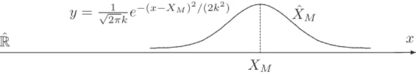
The distance on the stochastic line. The stochastic line is a line where the coordinates of the points are stochastic. This line will be denoted by ˆR. If on the real line a point M has the coordinate XM, on the stochastic line this corresponds to a stochastic point ˆM with stochastic
coordinate ˆXM = XM + ², with ² random variable normally distributed with mean zero and
standard deviation k, independent on the point. This way each point on the line corresponds to a normal distribution centered at the coordinate of that point, see Fig. 3. It worth noting that when k → 0 the distribution tends to the Dirac delta function δXM and the stochastic line becomes in this case the usual real line.
-XM ˆ XM x ˆ R y = √1 2πke −(x−XM)2/(2k2) ... ... ... ... ...... ...... ... .... ... .... ... .... ... .... ... .... ... .
Figure 3: Each point on the stochastic line corresponds to a normal distribution centered at the coordinate of that point.
Consider two stochastic points ˆM , ˆN on the stochastic line with the coordinates
ˆ
with ²M, ²N ∼ N (0, k) independent random variables. Let M and N denote the expected
positions of the aforementioned stochastic points. The distance between the points is the random variable | ˆM ˆN | = | ˆXM − ˆXN| = |(XM− XN) + (²M− ²N)| ∼ N (|XM− XN|, k √ 2), and hence E(| ˆM ˆN |) = |XM− XN| = |M N |,
which shows that the distance f ( ˆM , ˆN ) = | ˆM ˆN | is a stochastic invariant with the variance
E(| ˆM ˆN |2) −¡E(| ˆM ˆN |)¢2= |M N |2+ 2k2− |M N |2= 2k2.
This stochastic invariant explains why measuring a distance several times and averaging out the results yields a better approximation for the distance.
Invariants on the stochastic plane. The stochastic plane is a plane with all points stochastic, i.e. points for which the coordinates are random variables. The stochastic plane will be denoted
by ˆP to make the distinction from the real plane denoted by P. If ˆM is a stochastic point in
the plane, then its coordinates are ˆ
XM = XM + ²M, YMˆ = YM + ²0M,
where (XM, YM) are the coordinates of the expected point M = E( ˆM ). The random errors
are considered independent and normally distributed, with ² ∼ N (0, k), ²0∼ N (0, k0). Next we
shall provide a few examples of stochastic invariants of the plane.
The midpoint of a line segment. Let ˆA and ˆB be two stochastic points in the stochastic
plane. We can easily see that the coordinates of the midpoint of the line segment AB
fX( ˆA, ˆB) = 1
2( ˆXA+ ˆXB),
fY( ˆA, ˆB) = 1
2( ˆYA+ ˆYB)
are stochastic invariants. The variance of the first invariant is k2/2 and the variance of the
second one is k02/2.
The center of mass. Given a polygon with the vertices at the stochastic points ˆAi, i ∈
{1, . . . , n}, with the stochastic coordinates
ˆ
XAi = XAi+ ²i, YAˆ i= YAi+ ²
0
i,
then the coordinates of the center of mass
fX( ˆA1, . . . , ˆAi) = 1 n X ˆ XAi, fY( ˆA1, . . . , ˆAi) = 1 n X ˆ YAi
are stochastic invariants since E¡fX( ˆA1, . . . , ˆAi) ¢ = 1 n X E( ˆXAi) = 1 n X XAi= fX(A1, . . . , Ai) = fX ¡ E( ˆA1), . . . , E( ˆAn) ¢ .
Since ²1, . . . , ²n are independent and normally distributed with variance k2, then their
av-erage 1 n
P
²i has variance k2
n. It follows that fX( ˆA1, . . . , ˆAi) has variance k
2
n. Similarly,
fY( ˆA1, . . . , ˆAi) has variance k02
n . We notice that when n → ∞, the variance tends to zero,
which means that the coordinates of the center of mass tend to become deterministic in this limit case.
The angular argument. If ˆM is a stochastic point on the fixed unit circle, its angular
argument is given by τ = t + ², where ² ∼ N (0, k). Then f ( ˆM ) = τ is a stochastic invariant
with variance k2, since
E¡f ( ˆM )¢= E(τ ) = E(t + ²) = t = f¡E( ˆM )¢.
The inner product function. For any two stochastic points ˆM and ˆN in the plane ˆP define
f ( ˆM , ˆN ) = ˆXMXNˆ + ˆYMYNˆ .
A computation shows
f ( ˆM , ˆN ) = (XM+ ²M)(XN+ ²N) + (YM + ²0M)(YN + ²0N)
= XMXN+ YMYN+ ²NXM + ²MXN + ²M²N
+YM²0M + ²0MYN+ ²0M²0N,
and taking the expectation yields
E¡f ( ˆM , ˆN )¢= XMXN + YMYN = f (M, N ) = f
¡
E( ˆM ), E( ˆN )¢,
i.e. the function f is a stochastic invariant.
The area of a triangle. In the following we shall show that the area of a triangle is a
stochastic invariant. Consider three stochastic points ˆA, ˆB, ˆC with E( ˆA) = A, E( ˆB) = B,
E( ˆC) = C. Consider the oriented area function f : ˆP × ˆP × ˆP → R given by
f ( ˆA, ˆB, ˆC) = σ( ˆA, ˆB, ˆC) = 1 2 ¯ ¯ ¯ ¯ ¯ 1 XAˆ YAˆ 1 XˆB YˆB 1 XCˆ YCˆ ¯ ¯ ¯ ¯ ¯, where ˆ XA = XA+ ²A, XBˆ = XB+ ²B, XCˆ = XC+ ²C ˆ YA = YA+ ²A, YBˆ = YB+ ²B, YCˆ = YC+ ²C.
Using the linearity property of the determinant we have f ( ˆA, ˆB, ˆC) = 1 2 ¯ ¯ ¯ ¯ ¯ 1 XAˆ YAˆ 1 XBˆ YBˆ 1 XCˆ YCˆ ¯ ¯ ¯ ¯ ¯ = 1 2 ¯ ¯ ¯ ¯ ¯ 1 XA YA 1 XB YB 1 XC YC ¯ ¯ ¯ ¯ ¯+ 1 2 ¯ ¯ ¯ ¯ ¯ 1 XA ²0A 1 XB ²0B 1 XC ²0C ¯ ¯ ¯ ¯ ¯+ 1 2 ¯ ¯ ¯ ¯ ¯ 1 ²A YA 1 ²B YB 1 ²C YC ¯ ¯ ¯ ¯ ¯+ 1 2 ¯ ¯ ¯ ¯ ¯ 1 ²A ²0A 1 ²B ²0B 1 ²C ²0C ¯ ¯ ¯ ¯ ¯ = σ(A, B, C) +1 2∆1+ 1 2∆2+ 1 2∆3. (3.6)
The expected value of the last three determinants vanish. For instance,
E(∆1) = E "¯¯ ¯ ¯ ¯ 1 XA ²0A 1 XB ²0B 1 XC ²0C ¯ ¯ ¯ ¯ ¯ # = ¯ ¯ ¯ ¯ ¯ 1 XA E(²0A) 1 XB E(²0B) 1 XC E(²0C) ¯ ¯ ¯ ¯ ¯= ¯ ¯ ¯ ¯ ¯ 1 XA 0 1 XB 0 1 XC 0 ¯ ¯ ¯ ¯ ¯= 0. Then taking the expected value in relation (3.6) yields
E¡f ( ˆA, ˆB, ˆC)¢= σ(A, B, C) = f (A, B, C),
i.e. the oriented area of a triangle is a stochastic invariant. Next we shall compute its variance. Using (3.6) we get V arf = E¡f2( ˆA, ˆB, ˆC)¢− σ2(A, B, C) = 1 4E(∆ 2 1+ ∆22+ ∆23) + σ(A, B, C)E(∆1+ ∆2+ ∆3) +1 2E(∆1∆2+ ∆2∆3+ ∆3∆1). (3.7)
Expanding the determinant
∆1= XB(²0C− ²0A) + XA(²0B− ²0C) + XC(²0A− ²0B), and then ∆21 = XB2(²0C− ²0A)2+ XA2(²0B− ²0C)2+ XC2(²0A− ²0B)2 +2XAXB(²0 C− ²0A)(²0B− ²0C) + 2XBXC(²0C− ²0A)(²0A− ²0B) +2XAXC(²0 B− ²0C)(²0A− ²0B). Using E¡(²0 B− ²0C)2 ¢ = E¡(²0 A− ²0B)2 ¢ = E¡(²0 C− ²0A)2 ¢ = 2k02, E¡(²0 C− ²0A)(²0B− ²0C) ¢ = −E(²02 C) = −k02, E¡(²0 C− ²0A)(²0A− ²0B) ¢ = −E(²02 A) = −k02,
taking the expectation yields
E(∆2
1) = 2k02(XA2 + XB2 + XC2 − XAXB− XBXC− XCXA). (3.8)
Similarly we can show that
E(∆22) = 2k2(YA2+ YB2+ YC2− YAYB− YBYC− YCYA). (3.9)
Expanding the last determinant
∆3= ²B(²0C− ²0A) + ²A(²0B− ²0C) + ²C(²0A− ²0B)
and taking the square yields ∆2
3 = ²2B(²0C− ²0A)2+ ²2A(²B0 − ²0C)2+ ²C2(²0A− ²0B)2
= 2²B²A(²0C− ²0A)(²0B− ²0C) + 2²B²C(²0C− ²A0 )(²0A− ²0B) + 2²A²C(²B0 − ²0C)(²0A− ²0B).
Using the independence of the variables ² and ²0 we have
E¡²2 B(²0C− ²0A)2 ¢ = E(²2 B)E(²0C− ²0A)2= k2· 2k02, E¡²B²A(²0C− ²0A)(²0B− ²0C) ¢ = E(²B)E(²A)E ¡ (²0C− ²0A)(²0B− ²0C) ¢ = 0, and the similar relations. Then the previous relation yields
E(∆23) = 6k2k02.
Using the properties of independent random variables we also have
E(∆1∆2) = E(∆2∆3) = E(∆3∆1) = 0, E(∆1) = E(∆2) = E(∆3) = 0.
Substituting in formula (3.7) we obtain
V arf = 1 2k 02(X2 A+ XB2 + XC2 − XAXB− XBXC− XCXA) +1 2k 2(Y2 A+ YB2+ YC2− YAYB− YBYC− YCYA) + 3 2k 2k02.
To conclude, a good estimation of the area of a triangle with stochastic vertices is the area of the triangle formed by the centers of the distributions of the aforementioned stochastic vertices. Since any convex polygon can be partitioned into triangles, using that the area function is additive, we obtain that the signed area function associated with any convex polygon is a stochastic invariant.
Operations with stochastic invariants.It follows easily from the definition that the linear combination of two stochastic invariants is also a stochastic invariant. However, the usual product is not necessarily a stochastic invariant, but the tensorial product is.
Tensorial product of stochastic invariants. Let f ( ˆM1, . . . , ˆMr) and g( ˆN1, . . . , ˆNs) be two
stochas-tic invariants. Define the new stochasstochas-tic invariant
(f ⊗ g)( ˆM1, . . . , ˆMr, ˆN1, . . . , ˆNs) = f ( ˆM1, . . . , ˆMr)g( ˆN1, . . . , ˆNs). Using the independence we can check that
E[(f ⊗ g)( ˆM1, . . . , ˆMr, ˆN1, . . . , ˆNs)] = E[f ( ˆM1, . . . , ˆMr)]E[g( ˆN1, . . . , ˆNs)]
= f (M1, . . . , Mr)g(N1, . . . , Ns) = (f ⊗ g)(M1, . . . , Mr, N1, . . . , Ns).
4
Stochastic transforms
A mapping F = (F1, F2) : ˆP → ˆP is called a stochastic transform if its components F1, F2 : ˆ
P → ˆR are stochastic invariants. This means
E¡F ( ˆM )¢= F¡E( ˆM )¢, ∀ ˆM ∈ ˆP.
Next we shall encounter a few examples. Since E is a linear operator, then any transform with linear components is a stochastic transform. In particular, a translation, a rotation or an affine transform is a stochastic transform. For instance, if T is the translation by a fixed vector (u, v) given by
x0 = x + u
y0 = y + v
then
E¡T ( ˆXM, ˆYM)¢=¡E( ˆXM+u), E( ˆYM+v)¢=¡E( ˆXM)+u, E( ˆYM)+v¢= T¡E( ˆXM), E( ˆYM)¢.
Proposition 4.1 Let S denote the set of all the stochastic transforms of the plane ˆP. Then (i) If f, g ∈ S, then αf + βg ∈ S, for all α, β ∈ R.
(ii) If f, g ∈ S, then f ◦ g ∈ S.
Proof: (i) It comes from the linearity of the expectation operator E.
(ii) It follows from the commutativity between E and functions the f and g.
(iii) Applying the expectation to f¡f−1( ˆM )¢= ˆM yields E¡f (f−1( ˆM )¢= M , which after
using the commutativity between E and f yields
f¡E(f−1( ˆM ))¢= M.
Taking the inverse of f yields
E(f−1( ˆM )) = f−1(M ),
which is E(f−1( ˆM )) = f−1¡E( ˆM )¢, so f−1 ∈ S.
The invertible elements of S will be denoted by U (S). This forms a group of transforms which is noncommutative. For instance, as easily follows from the linearity, any transformation of the plane of type
x0 = ax + by + c 1 y0 = cx + dy + c2,
with ad 6= bc, is an element of U (S). We shall show in the following that there are elements of
U (S) which are not isometries nor affine transforms. In order to show this it suffices to provide
an example of a stochastic transform of the plane which is not linear.
A nonlinear stochastic transform. Consider F = (F1, F2) : ˆP = ˆR × ˆR → ˆP given by
F1(ˆx, ˆy) = exˆsin ˆy
F2(ˆx, ˆy) = exˆcos ˆy,
which is invertible since ∆(F1, F2) ∆(ˆx, ˆy) = −e
2ˆx6= 0. Consider the stochastic coordinates
ˆ
x = x + ², y = y + ²ˆ 0,
with ², ²0∼ N (0, k) independent variables.
We recall from section 2 that E(cos ²0) = e−k2/2
and E(sin ²0) = 0. Using a similar method
we shall show that E(e²) = ek2/2
. Since E(e²) = Rexϕ(x) dx, with ϕ(x) = √1
2πke
−x2/2k2
, the expected value E(e²) is uniquely determined by the density function ϕ(x), so if the random
variable ² is replaced by another one with the same density function, then the expected values are the same. We choose to replace ² by√k
tWt∼ N (0, k), where Wtstands for the 1-dimensional
Brownian motion. Denote √k
t= σt. Using (1.3) we have E(e²) = E¡ X σ n tWtn n! ¢ =X 1 n! ³ σ2 tt 2 ´n = etσ2t/2= ek2/2. Next we shall check that F1 is a stochastic invariant.
E¡F1(ˆx, ˆy)¢ = E(eˆxsin ˆy) = E¡exe²sin(y + ²0)¢
= exsin y E(e²cos ²0) + excos y E(e²sin ²0)
= exsin y E(e²)E(cos ²0) + excos y E(e²)E(sin ²0) = exsin y ek2/2 e−k2/2 + excos y ek2/2 · 0 = exsin y = F 1(x, y) = F1 ¡ E(ˆx), E(ˆy)¢.
Similarly one can show that E¡F2(ˆx, ˆy)¢= F2
¡
E(ˆx), E(ˆy)¢. It follows that F = (F1, F2) is a
stochastic transform, and F ∈ U (S).
Another example of nonlinear stochastic transform is F = (F1, F2) with
F1(ˆx, ˆy) = x − ˆˆ xˆy + ˆy
F2(ˆx, ˆy) = x + ˆˆ xˆy + ˆy,
which is invertible on ˆP\{(ˆx, ˆy)}. This follows from the linearity of E and the properties of ²
and ²0
E(ˆx ± ˆxˆy + ˆy) = x ± E(xy + x²0+ y² + ²²0) + y = x ± xy + y.
It is worth to notice that in the last two examples the components F1and F2are harmonic
functions, i.e., (∂2
x+ ∂y2)Fi(x, y) = 0, i = 1, 2. In the next section we shall deal with this
property of the stochastic transforms.
5
The main result on stochastic transforms
The first result deals with a characterization of the stochastic invariants on the stochastic line ˆ
R.
Theorem 5.1 f : ˆR → ˆR is a stochastic invariant if and only if f (x) is a linear function.
Proof: Let ˆx = x + ², with ² ∼ N (0,√t). We have
E¡f (x + ²)¢=
Z
f (u)ϕt(u − x) du =
Z
f (x + v)ϕt(v) dv.
Since f is a stochastic invariant
E¡f (x + ²)¢= f (x),
and hence
f (x) =
Z
Differentiating twice with respect to x and integrating by parts yields f00(x) = Z f00(x + v)ϕt(v) dv = Z f (x + v)∂v2ϕt(v) dv = 2 Z f (x + v)∂tϕt(v) dv = 2∂t Z f (x + v)ϕt(v) dv = 2∂tf (x) = 0,
and hence f (x) is linear in x.
The converse statement follows from the linearity of the expectation operator E. The next result extends the previous one to the 2-dimensional case.
Theorem 5.2 Let ˆP = ˆR × ˆR be the stochastic plane. Then F = (F1, F2) : ˆP → ˆP is a
stochastic transform if and only if the components F1 and F2 are harmonic functions, i.e.
(∂2
x+ ∂y2)Fi= 0, i = 1, 2.
Proof: Assume F = (F1, F2) is a stochastic transform. Let ˆx = x + ², ˆy = y + ²0, with
², ² ∼ N (0,√t), independent stochastic variables. Let ϕt(x) be the density function of a
normally distributed random variable with zero mean and variance t. It is known that this is the heat kernel for the operator ∂t−12∂2x, so
2∂tϕt(x) = ∂x2ϕt(x), t > 0. (5.10)
Since ˆx and ˆy are independent random variables, their joint distribution function is the product
of their density functions. Using this fact we have
E¡F1(ˆx, ˆy)¢ = ZZ F1(u, v)ϕt(u − x)ϕt(v − y) dudv = ZZ F1(w + x, z + y)ϕt(w)ϕt(z) dwdz.
Since F is a stochastic transform, E¡F1(ˆx, ˆy)¢= F1(x, y). Then the previous relation yields F1(x, y) =
ZZ
F1(w + x, z + y)ϕt(w)ϕt(z) dwdz.
Differentiating twice with respect to x and using integration by parts yields
∂x2F1(x, y) = ∂x2 ZZ F1(w + x, z + y)ϕt(w)ϕt(z) dwdz = ZZ F1(w + x, z + y)∂2 wϕt(w)ϕt(z) dwdz,
∂2 xF1(x, y) = 2 ZZ F1(w + x, z + y)∂tϕt(w)ϕt(z) dwdz. (5.11) Similarly we obtain ∂2 yF1(x, y) = 2 ZZ F1(w + x, z + y)ϕt(w)∂tϕt(z) dwdz. (5.12)
Adding (5.11) and (5.12) we get 1 2 ¡ ∂2 x+ ∂y2 ¢ F1(x, y) = ZZ F1(w + x, z + y)∂t ¡ ϕt(w)ϕt(z) ¢ dwdz = ∂t ZZ F1(w + x, z + y)¡ϕt(w)ϕt(z) ¢ dwdz = ∂tE¡F1(ˆx, ˆy)¢= ∂tF1(x, y) = 0,
and hence F1 is a harmonic function. Similar considerations apply to the component F2.
In order to prove the converse, we assume the functions Fi harmonic and show that F is a
stochastic transform. It suffices to show that the components Fi are stochastic invariants.
We make the remark that the definition property of the stochastic invariant f : ˆR × ˆR → ˆR
E(f (ˆx)) = f (E(ˆx))
corresponds to the mean property of the harmonic functions. If ˆx ∈ ˆR × ˆR is a Gaussian random variable centered at x, then E(f (ˆx)) is the average of f (ˆx) over the entire stochastic plane. For f harmonic we have
E(f (ˆx)) = average(f (ˆx)) = lim
R→∞ 1 πR2 Z |u−x|≤R f (u) du = f (x) = f (E(ˆx)).
Applying this argument can be applied for f = Fi, i = 1, 2, shows that Fi are stochastic
invariants.
Corollary 5.3 Any stochastic transform F = (F1, F2) has analytic components.
Proof: It follows from the fact that harmonic functions on R2 are real parts of holomorphic
functions.
Corollary 5.4 Let U be an open set in the plane. If F and H are two stochastic transforms
with F|U = H|U, then F = H.
6
The geometry induced by U(S)
We are interested in the study of those properties of the plane that remain unchanged when the points of the plane are subject to the transformations of the group U (S). If Isom is the isometries group of the plane, then Isom is a proper subgroup of U (S), and hence all the properties invariant by U (S) are also invariant by Isom.
Next we shall provide an example of a class of transformations of U (S).
Proposition 6.1 Let F = (F1, F2) : R2 → R2 be a nonconstant function which satisfies the Cauchy-Riemann system of equations
∂F1 ∂x = ∂F2 ∂y ∂F1 ∂y = − ∂F2 ∂x . Then F ∈ U (S).
Proof: Using the Cauchy-Riemann equations we have
∂2F1 ∂x2 + ∂2F1 ∂y2 = ∂ ∂x ∂F2 ∂y − ∂ ∂y ∂F2 ∂x = 0,
so F1 is harmonic. In a similar way F2 is harmonic. In order to show that F is invertible we
compute its Jacobian using the Cauchy-Riemann equations
|JF| = ¯ ¯ ¯ ¯ ¯ ∂F1 ∂x ∂F∂x2 ∂F1 ∂y ∂F∂y2 ¯ ¯ ¯ ¯ ¯= ³ ∂F1 ∂x ´2 +³ ∂F1 ∂y ´2 =³ ∂F2 ∂x ´2 +³ ∂F2 ∂y ´2 6= 0.
If consider R2 = C and write F = F
1+ iF2, then F becomes a biholomorphic function.
It is known that the biholomorphic transforms are conformal, i.e. preserve angles between lines and curves. Hence a transformation given by the Proposition 6.1 preserves angles. For instance, if choose the holomorphic function F (z) = ez = ex+iy = excos y + iexsin y, then
F = (F1, F2) = (excos y, exsin y) is a stochastic transform which preserves angles.
7
Stochastic invariants and Brownian motions
Assume that the coordinates of the stochastic point ˆM change with respect to time t according
to the laws
ˆ
where W1(t), W2(t) are independent 1-dimensional Brownian motions starting at 0. Consider
the stochastic transform F = (F1, F2) : ˆP → ˆP. The stochastic point F ( ˆM ) has the coordinates
(ˆut, ˆvt) =¡F1(ˆxt, ˆyt), F2(ˆxt, ˆyt)
¢
.
Applying Ito’s formula yields
dut = ∂F1 ∂x dW1(t) + ∂F1 ∂y dW2(t) + 1 2 Ã ∂2F1 ∂x2 + ∂2F1 ∂y2 ! dt dvt = ∂F2 ∂x dW1(t) + ∂F2 ∂y dW2(t) + 1 2 Ã ∂2F2 ∂x2 + ∂2F2 ∂y2 ! dt.
Since the functions F1, F2 are harmonic, see Theorem 5.2, we have
dˆut = ∂F1 ∂x dW1(t) + ∂F1 ∂y dW2(t) dˆvt = ∂F2 ∂x dW1(t) + ∂F2 ∂y dW2(t),
which after integration yields ˆ ut = u0ˆ + Z t 0 ∂F1 ∂x dW1(s) + Z t 0 ∂F1 ∂y dW2(s) (7.13) ˆ vt = ˆv0+ Z t 0 ∂F2 ∂x dW1(s) + Z t 0 ∂F2 ∂y dW2(s), (7.14)
which are the coordinates of the point F ( ˆM ). Since the Ito integral is a martingale, these
coordinates satisfy
E(ˆut, ˆvt) = (ˆu0, ˆv0) = (x, y) = F¡E( ˆM )¢.
Moreover, the coordinates (7.13–7.14) represent versions of the 1-dimensional Brownian motions starting at (x, y) with a certain time scale. Applying Corollary 8.5.3 of [2], p. 154 yields
ˆ ut= x + W1 ¡ α1(t)¢, ˆvt= y + W2 ¡ α2(t)¢, with αi(βi(t)) = βi(αi(t)) = t, t ≥ 0, where βi(t) = Z t 0 k∇Fik2(W 1(s), W2(s)) ds.
In the particular case when F = F1+ iF2is holomorphic, then after a certain change of the
time scale the process (ˆut, ˆvt) becomes a 2-dimensional Brownian motion, see [2], p. 158. For more properties of Brownian motion the reader may consult [3] and [1].
References
[1] Kuo, H.H.: Introduction to Stochastic Integration, Springer, Universitext, 2006.
[2] Øksendal, B.: Stochastic Differential Equations, An Introduction with Applications, 6th ed., Springer-Verlag Berlin Heidelberg New-York, 2003.
[3] Ross, S. M.: Stochastic Processes, 2nd edition, John Wiley & Sons, Inc., 1996.
Ovidiu Calin
Eastern Michigan University Department of Mathematics Ypsilanti, MI, 48197, USA [email protected] Der-Chen Chang Georgetown University Department of Mathematics Washington, DC, USA [email protected]