以記憶體追蹤方式在單指令多執行緒架構中資料分享程度之分析研究

National Chiao Tung University

EECS International Graduate Program

Thesis

記憶體追蹤方式在單指令多執行緒架構中資料分享程度之分析研

究

A Memory Trace-Based Analysis for Data Sharing Degree in SIMT

Architectures

Student: Luis Angel Garrido Platero

Advisor: Prof. Bo-Cheng Lai

以記憶體追蹤方式在單指令多執行緒架構中資料分享程度之分析

研究

A Memory Trace-Based Analysis for Data Sharing Degree in SIMT

Architectures

研 究 生：盧以斯

Student: Luis Angel Garrido Platero

指導教授：賴伯承

Advisor: Bo-Cheng Lai

國 立 交 通 大 學

EECS International Graduate Program

碩 士 論 文

A Thesis

Submitted to the EECS International Graduate Program National Chiao Tung University

in partial Fulfillment of the Requirements for the Degree of

Master in

EECS

June 2013

Hsinchu, Taiwan, Republic of China

i

以記憶體追蹤方式在單指令多執行緒架構中資料分享程度之分析

研究

Student:

Advisors:

EECS International Graduate Program

National Chiao Tung University

CHINESE ABSTRACT

在本論文中，我們透過量化單一指令多執行續程式中記憶體存取的資料分

享程度進而分析應用程式的區域特性。此外，我們也提供了不同執行環境

下之資料分享的視覺化方法。為了量化資料分享程度，本論文使用含有執

行階段記憶體位置的記憶體追蹤以完成記憶體存取的資料分享程度分析。

在此分析中，我們重新定義重複使用距離的概念以提供分析以及不同執行

環境的需要。

ii

A Memory Trace-based Analysis for Data Sharing Degree of SIMT Architectures

Student:

Advisors: Dr.

EECS International Graduate Program

National Chiao Tung University

ENGLISH ABSTRACT

In this work, we address the problem of quantifying the data sharing degree of

the memory access behavior within specific SIMT applications in order to

quantify the locality characteristics of the application‟s workload. In addition,

we also offer way to visualize the way the sharing patterns of the applications

and the way they change under different models of runtime scenarios. For the

purposes of quantifying the data sharing degree a memory trace is generated that

contains information of the addresses accessed at a specific point of execution.

Then, the information contained in the traces is used to perform the data sharing

degree analysis of memory accesses. In this analysis, we have redefined the

reuse distance concept in order to make it suitable to our analytical requirements,

at the same time considering the particulars of the execution model previously

mentioned.

iii

TABLE OF CONTENTS

Chinese Abstract………..i

English Abstract...ii

Table of Contents………..……….iii

List of Tables………...iv

List of Figures………...v

Symbols………...xvi

I. INTRODUCTION ... 1

II. OVERVIEW OF SIMT PROCESSORS ... 6

2.1 Hardware of GPU Architectures... 6

2.2 Programming and execution abstractions of GPU ... 7

2.3 Memory Hierarchy of GPUs ... 8

III. LOCALITY ANALYSES IN CMP AND UNIPROCESSOR SYSTEMS ... 9

IV. DATA REUSE CHARACTERIZATION ... 12

4.1 Definition of the Data Reuse Degree ... 12

4.1 Definition of the Reuse Distance ... 14

4.1.1 Traditional reuse distance analyses ... 15

4.1.2 Reuse Distance for SIMT Processors ... 18

V. ANALYSIS METHODOLOGY FOR DATA REUSE CHARACTERIZATION ... 21

VI. SCENARIOS FOR DATA REUSE CHARACTERIZATION ... 26

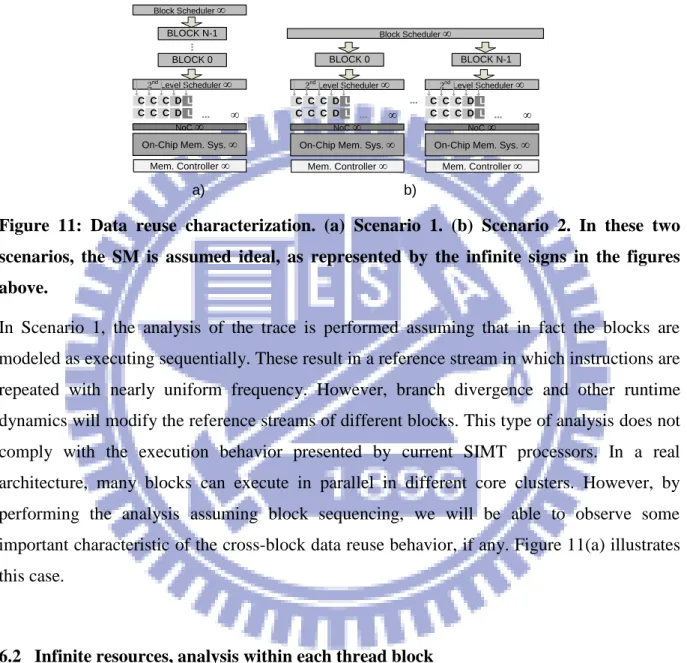
5.1 Infinite resources, thread blocks are modeled as executing sequentially ... 27

5.2 Infinite resources, analysis within each thread block ... 27

5.3 Infinite resources, all thread are modeled as executing in parallel ... 28

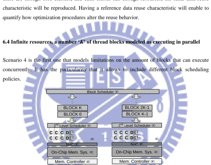
5.4 Infinite resources, a number „K‟ of thread blocks modeled as executing in parallel ... 29

iv

5.5 Limited resources, „K‟ block modeled as executing

in parallel, within core cluster analysis ... 31

5.6 Limited resources, „K‟ blocks modeled as executing in parallel, inter-core cluster ... 33

VII. EXPERIMENTATION FRAMEWORK ... 35

6.1 Trace Generation Stage ... 35

6.2 Reference Stream Analysis Stage ... 36

6.2.1 Model for Thread Blocks ... 36

6.2.2 Scheduling Policies ... 39

6.2.3 Core cluster modeling ... 43

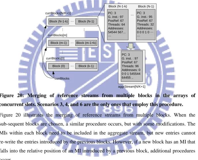
6.2.4 Merging of reference streams ... 44

6.2.5 Adjusting the position index of Mis ... 48

6.2.6 Locality Analyzer Architecture: Putting it all together ... 50

VIII. APPLICATION OPTIMIZATION ... 52

8.1 Thread Mapping Methodology ... 52

IX. EXPERIMENTAL RESULTS ... 55

9.1 Data Reuse Characteristic with serialized blocks and on a per block basis ... 55

9.2 Data Reuse Characteristic with varying parallelism capabilities ... 64

9.3 Data Reuse Characteristic with limitations of SIMT Architectures ... 73

9.4 Data Reuse Characteristic when applying code optimizations ... 86

X. RELATED WORK ... 98

XI. CONCLUSIONS ... 101

v

LIST OF TABLES

vi

LIST OF FIGURES

Figure 1: Benefits obtained when taking advantage of the data reuse in SIMT applications. (a) DRAM memory transactions with and without coalescing. The first two cases from the top illustrate the case for coalescing. The last case shows the case when coalescing is not possible. (b) Illustration of the contention effect in a CMP. ... 3 Figure 2: Diagram of a core cluster based on NVIDIA's Kepler GeForce GTX 680 GPU. (a) The core cluster with its internal hardware modules. (b) Illustration of the thread hierarchy in the SIMT programming model. ... 6 Figure 3: Reuse distance concept and memory instruction reuse behavior in SIMT programs. (a) Sample measurement of reuse distance in traditional multiprocessors. (b) Reuse distance behavior in SIMT architectures. ... 10 Figure 4: A sample stream of memory instructions. The instruction array appears in the left column, the address array is presented in the middle column and the Reuse Degree for memory instructions „i‟ „i+2‟ and „i+2‟ „i+4‟ appears in the right column. ... 13 Figure 5: Reuse distance analysis as applied in uniprocessor systems. (a) Sample memory trace. (b) Changes of the state of the stack as memory instructions are issued. ... 15 Figure 6: Reuse distance analysis in CMP systems with private memory subsystem. (a) Sample reference stream. (b) Stacks for the private memory subsystem. ... 16 Figure 7: Reuse distance analysis in CMPs with shared memory subsystem. (a) Sample reference stream. (b) Stacks for each memory subsystem... 17 Figure 8: Data reuse degree in a sample reference stream of a SIMT processor with „N‟ processing cores. (a) Sample reference stream of a SIMT processor. (b) Data Reuse Degree for memory instructions „i‟ ‟i+k‟ and „i+2‟ ‟i+2+k‟. ... 19 Figure 9: Limitations when performing the baseline methodology for reuse distance analysis on SIMT processors. (a) Subset of the reference stream as it appears in Figure 7. (b) Possible ways to arrange the accessed addresses on the stacks. ... 22 Figure 10: Flow chart of the data reuse characterization methodology. This flow chart shows all the steps when performing the analysis over a reference stream. ... 23

vii

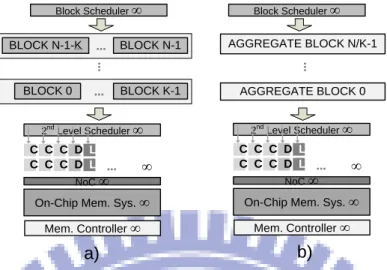
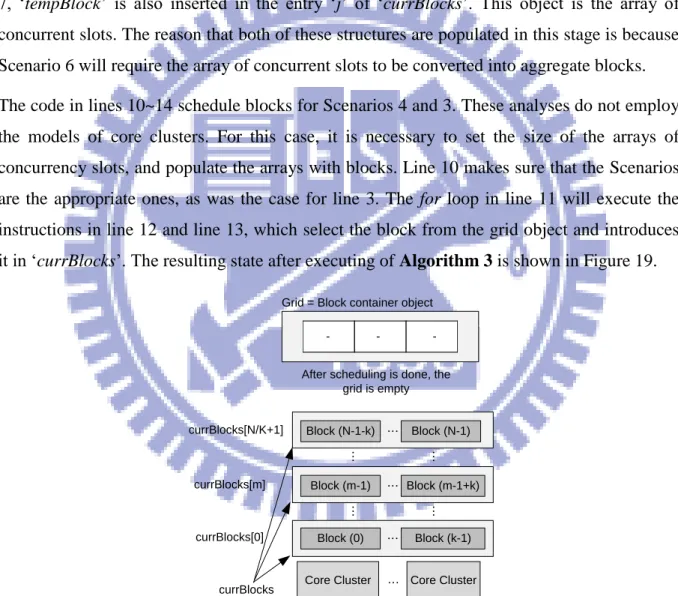
Figure 11: Data reuse characterization. (a) Scenario 1. (b) Scenario 2. In these two scenarios, the SM is assumed ideal, as represented by the infinite signs in the figures above. ... 27 Figure 12: Scenario 3 of data reuse characterization assuming ideal core clusters. (a) Illustrates the way blocks are intended to be executed. (b) Illustrates the Aggregate Block that results from merging the streams of all CTAs. ... 28 Figure 13: Scenario 4 of the reuse degree characterization. Only 'K' blocks are modeled as executing concurrently. This is equivalent as having 'K' ideal core clusters, each one executing one block at the time. ... 29 Figure 14: (a) An ideal core cluster executing the reference streams of 'K' parallel blocks. (b) The streams of parallel blocks merged into a series of aggregate blocks, executed in sequence. ... 30 Figure 15: Scenario 5 of the data reuse characterization analysis. Each core cluster has now a finite number of load/store instructions. The analysis is performed within each core cluster. 32 Figure 16: Scenario 6 of the data reuse characterization. The analysis is performed over the aggregate of the reference streams in every core cluster. The number of load/store units is the total sum across the core clusters. ... 33 Figure 17: Formation of Block objects within the Locality Analyzer. The block objects contain their individual reference stream which consists on a series of ordered MIs. Each MI has access information of its own. ... 37 Figure 18: Block scheduling module and block scheduling flow (a) Block scheduling module assigning blocks to a system with one core cluster. (b) Block scheduling module assigning blocks to a system with multiple core clusters ... 40 Figure 19: After assigning blocks to the core clusters. The blocks are queued in each cluster, and are also inserted into the „currBlocks‟ structure, which represents the arrays of concurrent slots. ... 42 Figure 20: Merging of reference streams from multiple blocks in the arrays of concurrent slots. Scenarios 3, 4, and 6 are the only ones that employ this procedure. ... 45 Figure 21: The resulting reference stream of the aggregate blocks. It is possible to compare this with the streams shown in Figure 19. Notice how the „Addresses‟ and „Threads‟ fields are augmented ... 48

viii

Figure 22: Modifications of the position reference index within the reference stream. The value of the index of the MIs in streams other than the first will depend on the stream length of the streams before the current one. ... 49 Figure 23: Block diagram of the architecture of the Locality Analyzer. This is a very general and simplified version of our framework ... 50 Figure 24: Data reuse characteristic when modeling block execution sequentially for sta. (a) Full reuse characteristic. (b) Showing the reuse characteristic for the range RD={1, 400}. (c) Showing the reuse characteristic for the range RD={1, 100}. Notice the particular patterns. . 56 Figure 25: Data reuse characteristic when modeling block execution sequentially for gsim. (a) Full reuse characteristic. (b) Showing the reuse characteristic for the range RD={1, 400}. (c) Showing the reuse characteristic for the range RD={1, 100}. ... 56 Figure 26: Data reuse characteristic when modeling block execution sequentially for bfs. (a) Full reuse characteristic. (b) Showing the reuse characteristic for the range RD={1, 400}. (c) Showing the reuse characteristic for the range RD={1, 100}. ... 57 Figure 27: Data reuse characteristic when modeling block execution sequentially for

vectoradd. (a) Full reuse characteristic. (b) Showing the reuse characteristic for the range RD={1, 400}. (c) Showing the reuse characteristic for the range RD={1, 100}. ... 57

Figure 28: Source code for the kernels of bfs (a) and sta (b). ... 57 Figure 29: Data reuse characteristic on a per block basis for sta. (a) Data reuse characteristic for thread block 0. (b) Full reuse characteristic for thread block 1. ... 58 Figure 30: Data reuse characteristic on a per block basis for gsim. (a) Data reuse characteristic for thread block 0. (b) Full reuse characteristic for thread block 1. ... 58 Figure 31: Data reuse characteristic on a per block basis for bfs. (a) Data reuse characteristic for thread block 0. (b) Full reuse characteristic for thread block 1. ... 59 Figure 32: Data reuse characteristic on a per block basis for vectoradd. (a) Data reuse characteristic for thread block 0. (b) Full reuse characteristic for thread block 1. ... 59 Figure 33: Data reuse characteristic on a per block basis for nbf. (a) Data reuse characteristic for thread block 0. (b) Full reuse characteristic for thread block 1. ... 59

ix

Figure 34: Data reuse characteristic on a per block basis for moldyn. (a) Data reuse characteristic for thread block 0. (b) Full reuse characteristic for thread block 1. ... 60 Figure 35: Data reuse characteristic on a per block basis for irreg. (a) Data reuse characteristic for thread block 0. (b) Full reuse characteristic for thread block 1. ... 60 Figure 36: Data reuse characteristic on a per block basis for euler. (a) Data reuse characteristic for thread block 0. (b) Full reuse characteristic for thread block 1. ... 60 Figure 37: Data reuse characteristic when modeling block execution when all blocks run in parallel for sta. ... 64 Figure 38: Data reuse characteristic when modeling block execution when all blocks run in parallel for gsim. ... 65 Figure 39: Data reuse characteristic when modeling block execution when all blocks run in parallel for bfs. ... 65 Figure 40: Data reuse characteristic when all blocks of vectoradd are modeled as executing in parallel. ... 65 Figure 41: Data reuse characteristic when all blocks of nbf are modeled as executing in parallel. ... 66 Figure 42: Data reuse characteristic when all blocks of moldyn are modeled as executing in parallel. ... 66 Figure 43: Data reuse characteristic when all blocks of irreg are modeled as executing in parallel. ... 66 Figure 44: Data reuse characteristic when all blocks of euler are modeled as executing in parallel. ... 67 Figure 45: Data reuse characteristic when only „K‟ blocks of sta are modeled as executing in parallel. (a) Data reuse characteristic for K=2. (b) Data reuse characteristic for K=4. (c) Data reuse characteristic for K=8. (d) Data reuse characteristic for K=16. ... 68

x

Figure 46: Data reuse characteristic when only „K‟ blocks of gsim are modeled as executing in parallel. (a) Data reuse characteristic for K=2. (b) Data reuse characteristic for K=4. (c) Data reuse characteristic for K=8. (d) Data reuse characteristic for K=16. ... 68 Figure 47: Data reuse characteristic when only „K‟ blocks of bfs are modeled as executing in parallel. (a) Data reuse characteristic for K=2. (b) Data reuse characteristic for K=4. (c) Data reuse characteristic for K=8. (d) Data reuse characteristic for K=16. ... 69 Figure 48: Data reuse characteristic when only „K‟ blocks of vectoradd are modeled as executing in parallel. (a) Data reuse characteristic for K=2. (b) Data reuse characteristic for

K=4. (c) Data reuse characteristic for K=8. (d) Data reuse characteristic for K=16. ... 69

Figure 49: Data reuse characteristic when only „K‟ blocks of nbf are modeled as executing in parallel. (a) Data reuse characteristic for K=2. (b) Data reuse characteristic for K=4. (c) Data reuse characteristic for K=8. (d) Data reuse characteristic for K=16. ... 70 Figure 50: Data reuse characteristic when only „K‟ blocks of moldyn are modeled as executing in parallel. (a) Data reuse characteristic for K=2. The reuse domain for this case is actually RD={1,124030}. The tool used to make the graphs could not display it properly. (b) Data reuse characteristic for K=4. (c) Data reuse characteristic for K=8. (d) Data reuse characteristic for K=16. ... 70 Figure 51: Data reuse characteristic when only „K‟ blocks of irreg are modeled as executing in parallel. (a) Data reuse characteristic for K=2. (b) Data reuse characteristic for K=4. (c) Data reuse characteristic for K=8. (d) Data reuse characteristic ... 71 Figure 52: Data reuse characteristic when only „K‟ blocks of euler are modeled as executing in parallel. (a) Data reuse characteristic for K=2. The reuse domain for this case is actually RD={1,66623}. The tool used to make the graphs could not display it properly. (b) Data reuse characteristic for K=4. (c) Data reuse characteristic for K=8. (d) Data reuse characteristic ... 71 Figure 53: Data reuse characteristic resulting when only K=2 blocks of sta are modeled as executing in parallel. (a) Data reuse characteristic presented for reuse distance range RD={1,

20}. (b) Data reuse characteristic presented for reuse distance range RD={21, 40}. (c) Data

reuse characteristic presented for reuse distance range RD={41, 60}. ... 73 Figure 54: Data reuse characteristic resulting when only K=16 blocks of sta are modeled as executing in parallel. (a) Data reuse characteristic presented for reuse distance range RD={1,

20}. (b) Data reuse characteristic presented for reuse distance range RD={21, 40}. (c) Data

xi

Figure 55: Data reuse characteristic from the aggregate reference stream of all core clusters with varying number of load/store units in each core cluster for sta. (a) Data reuse characteristic for 16 load/store units per core cluster. (b) Data reuse characteristic for 32 load/store units per core cluster. (c) Data reuse characteristic for 64 load/store units per core cluster. ... 74 Figure 56: Data reuse characteristic from the aggregate reference stream of all core clusters with varying number of load/store units in each core cluster for gsim. (a) Data reuse characteristic for 16 load/store units per core cluster. (b) Data reuse characteristic for 32 load/store units per core cluster. (c) Data reuse characteristic for 64 load/store units per core cluster. ... 74 Figure 57: Data reuse characteristic from the aggregate reference stream of all core clusters with varying number of load/store units in each core cluster for bfs. (a) Data reuse characteristic for 16 load/store units per core cluster. (b) Data reuse characteristic for 32 load/store units per core cluster. (c) Data reuse characteristic for 64 load/store units per core cluster. ... 74 Figure 58: Data reuse characteristic from the aggregate reference stream of all core clusters with varying number of load/store units in each core cluster for vectoradd. (a) Data reuse characteristic for 16 load/store units per core cluster. (b) Data reuse characteristic for 32 load/store units per core cluster. (c) Data reuse characteristic for 64 load/store units per core cluster. ... 75 Figure 59: Data reuse characteristic from the aggregate reference stream of all core clusters with varying number of load/store units in each core cluster for nbf. (a) Data reuse characteristic for 16 load/store units per core cluster. (b) Data reuse characteristic for 32 load/store units per core cluster. (c) Data reuse characteristic for 64 load/store units per core cluster. ... 75 Figure 60: Data reuse characteristic from the aggregate reference stream of all core clusters with varying number of load/store units in each core cluster for irreg. (a) Data reuse characteristic for 16 load/store units per core cluster. (b) Data reuse characteristic for 32 load/store units per core cluster. (c) Data reuse characteristic for 64 load/store units per core cluster. ... 76 Figure 61: Data reuse characteristic from the aggregate reference stream of all core clusters with varying number of load/store units in each core cluster for euler. (a) Data reuse characteristic for 16 load/store units per core cluster. (b) Data reuse characteristic for 32 load/store units per core cluster. (c) Data reuse characteristic for 64 load/store units per core cluster. ... 76

xii

Figure 62: Data reuse characteristic in reuse distance range RD={0, 100} of the aggregate reference stream of all core clusters with varying number of load/store units for sta. (a) Data reuse characteristic for 16 load/store units per core cluster. (b) Data reuse characteristic for 32 load/store units per core cluster. (c) Data reuse characteristic for 64 load/store units per core cluster. ... 77 Figure 63: Data reuse characteristic from the reference stream of the first and second core clusters with varying number of load/store units for sta. (a) First core cluster with 16 load/store units. (b) Second core cluster with 16 load/store units. (c) First core cluster with 32 load/store units. (d) Second core cluster with 32 load/store units. (e) First core cluster with 64 load/store units. (f) Second core cluster with 64 load/store units. ... 79 Figure 64: Data reuse characteristic from the reference stream of the first and second core clusters with varying number of load/store units for gsim. (a) First core cluster with 16 load/store units. (b) Second core cluster with 16 load/store units. (c) First core cluster with 32 load/store units. (d) Second core cluster with 32 load/store units. (e) First core cluster with 64 load/store units. (f) Second core cluster with 64 load/store units. ... 80 Figure 65: Data reuse characteristic from the reference stream of the first and second core clusters with varying number of load/store units for bfs. (a) First core cluster with 16 load/store units. (b) Second core cluster with 16 load/store units. (c) First core cluster with 32 load/store units. (d) Second core cluster with 32 load/store units. (e) First core cluster with 64 load/store units. (f) Second core cluster with 64 load/store units. ... 81 Figure 66: Data reuse characteristic from the reference stream of the first and second core clusters with varying number of load/store units for vectoradd. (a) First core cluster with 16 load/store units. (b) Second core cluster with 16 load/store units. (c) First core cluster with 32 load/store units. (d) Second core cluster with 32 load/store units. (e) First core cluster with 64 load/store units. (f) Second core cluster with 64 load/store units. ... 82 Figure 67: Data reuse characteristic from the reference stream of the first and second core clusters with varying number of load/store units for nbf. (a) First core cluster with 16 load/store units. (b) Second core cluster with 16 load/store units. (c) First core cluster with 32 load/store units. (d) Second core cluster with 32 load/store units. (e) First core cluster with 64 load/store units. (f) Second core cluster with 64 load/store units. ... 83 Figure 68: Data reuse characteristic from the reference stream of the first and second core clusters with varying number of load/store units for moldyn. (a) First core cluster with 16 load/store units. (b) Second core cluster with 16 load/store units. (c) First core cluster with 32 load/store units. (d) Second core cluster with 32 load/store units. (e) First core cluster with 64 load/store units. (f) Second core cluster with 64 load/store units. ... 84

xiii

Figure 69: Data reuse characteristic from the reference stream of the first and second core clusters with varying number of load/store units for irreg. (a) First core cluster with 16 load/store units. (b) Second core cluster with 16 load/store units. (c) First core cluster with 32 load/store units. (d) Second core cluster with 32 load/store units. (e) First core cluster with 64 load/store units. (f) Second core cluster with 64 load/store units. ... 85 Figure 70: Data reuse characteristic from the reference stream of the first and second core clusters with varying number of load/store units for euler. (a) First core cluster with 16 load/store units. (b) Second core cluster with 16 load/store units. (c) First core cluster with 32 load/store units. (d) Second core cluster with 32 load/store units. (e) First core cluster with 64 load/store units. (f) Second core cluster with 64 load/store units. ... 86 Figure 71: Data reuse characteristic for block 0 of sta after coding optimizations. (a) After applying thread clustering. (b) After applying thread and warp clustering. (c) After applying thread clustering, warp clustering and block scheduling. (d) Comparison prior to optimizations and after thread clustering. Difference in the reuse degree is 17. (e) Comparison prior to optimizations and after thread and warp clustering. Difference in the reuse degree is 802. (f) Comparison prior to optimizations and after thread clustering, warp clustering and block scheduling. Difference in the reuse degree is 802. ... 87 Figure 72: Data reuse characteristic for block 0 of gsim after coding optimizations. (a) After applying thread clustering. (b) After applying thread and warp clustering. (c) After applying thread clustering, warp clustering and block scheduling. (d) Comparison prior to optimizations and after thread clustering. Difference in the reuse degree is 400. (e) Comparison prior to optimizations and after thread and warp clustering. Difference in the reuse degree is 795. (f) Comparison prior to optimizations and after thread clustering, warp clustering and block scheduling. Difference in the reuse degree is 794. ... 87 Figure 73: Data reuse characteristic for block 0 of bfs after coding optimizations. (a) After applying thread clustering. (b) After applying thread and warp clustering. (c) After applying thread clustering, warp clustering and block scheduling. (d) Comparison prior to optimizations and after thread clustering. Difference in the reuse degree is 17. (e) Comparison prior to optimizations and after thread and warp clustering. Difference in the reuse degree is 802 (f) Comparison prior to optimizations and after thread clustering, warp clustering and block scheduling. Difference in the reuse degree is 802. ... 88 Figure 74: Data reuse characteristic for block 0 of nbf after coding optimizations. (a) After applying thread clustering. (b) After applying thread and warp clustering. (c) After applying thread clustering, warp clustering and block scheduling. (d) Comparison prior to optimizations and after thread clustering. Difference in the reuse degree is 44458. (e) Comparison prior to optimizations and after thread and warp clustering. Difference in the reuse degree is 60346 (f) Comparison prior to optimizations and after thread clustering, warp clustering and block scheduling. Difference in the reuse degree is 60576. ... 88

xiv

Figure 75: Data reuse characteristic for block 0 of moldyn after coding optimizations. (a) After applying thread clustering. (b) After applying thread and warp clustering. (c) After applying thread clustering, warp clustering and block scheduling. (d) Comparison prior to optimizations and after thread clustering. Difference in the reuse degree is 352556. (e) Comparison prior to optimizations and after thread and warp clustering. Difference in the reuse degree is 446146. (f) Comparison prior to optimizations and after thread clustering, warp clustering and block scheduling. Difference in the reuse degree is 447102. ... 89 Figure 76: Data reuse characteristic for block 0 of irreg after coding optimizations. (a) After applying thread clustering. (b) After applying thread and warp clustering. (c) After applying thread clustering, warp clustering and block scheduling. (d) Comparison prior to optimizations and after thread clustering. Difference in the reuse degree is 47309. (e) Comparison prior to optimizations and after thread and warp clustering. Difference in the reuse degree is 53448. (f) Comparison prior to optimizations and after thread clustering, warp clustering and block scheduling. Difference in the reuse degree is 43212. ... 90 Figure 77: Data reuse characteristic for block 0 of euler after coding optimizations. (a) After applying thread clustering. (b) After applying thread and warp clustering. (c) After applying thread clustering, warp clustering and block scheduling. (d) Comparison prior to optimizations and after thread clustering. Difference in the reuse degree is 59694. (e) Comparison prior to optimizations and after thread and warp clustering. Difference in the reuse degree is 81755. (f) Comparison prior to optimizations and after thread clustering, warp clustering and block scheduling. Difference in the reuse degree is 82204. ... 90 Figure 78: Data reuse characteristic for all blocks running in parallel of sta after coding optimizations. (a) After applying thread clustering. (b) After applying thread and warp clustering. (c) After applying thread clustering, warp clustering and block scheduling. (d) Comparison prior to optimizations and after thread clustering. Difference in the reuse degree is -10216. (e) Comparison prior to optimizations and after thread and warp clustering. Difference in the reuse degree is 14229. (f) Comparison prior to optimizations and after thread clustering, warp clustering and block scheduling. Difference in the reuse degree is 11940. ... 92 Figure 79: Data reuse characteristic for all blocks running in parallel of gsim after coding optimizations. (a) After applying thread clustering. (b) After applying thread and warp clustering. (c) After applying thread clustering, warp clustering and block scheduling. (d) Comparison prior to optimizations and after thread clustering. Difference in the reuse degree is 8236. (e) Comparison prior to optimizations and after thread and warp clustering. Difference in the reuse degree is 21363. (f) Comparison prior to optimizations and after thread clustering, warp clustering and block scheduling. Difference in the reuse degree is 17129. ... 93 Figure 80: Data reuse characteristic for all blocks running in parallel of bfs after coding optimizations. (a) After applying thread clustering. (b) After applying thread and warp

xv

clustering. (c) After applying thread clustering, warp clustering and block scheduling. (d) Comparison prior to optimizations and after thread clustering. Difference in the reuse degree is -10812. (e) Comparison prior to optimizations and after thread and warp clustering. Difference in the reuse degree is 13361. (f) Comparison prior to optimizations and after thread clustering, warp clustering and block scheduling. Difference in the reuse degree is 11324. ... 93 Figure 81: Data reuse characteristic for all blocks running in parallel of nbf after coding optimizations. (a) After applying thread clustering. (b) After applying thread and warp clustering. (c) After applying thread clustering, warp clustering and block scheduling. (d) Comparison prior to optimizations and after thread clustering. Difference in the reuse degree is 6053. (e) Comparison prior to optimizations and after thread and warp clustering. Difference in the reuse degree is 7400. (f) Comparison prior to optimizations and after thread clustering, warp clustering and block scheduling. Difference in the reuse degree is 9138. ... 94 Figure 82: Data reuse characteristic for all blocks running in parallel of moldyn after coding optimizations. (a) After applying thread clustering. (b) After applying thread and warp clustering. (c) After applying thread clustering, warp clustering and block scheduling. (d) Comparison prior to optimizations and after thread clustering. Difference in the reuse degree is -3373236. (e) Comparison prior to optimizations and after thread and warp clustering. Difference in the reuse degree is -5170268. (f) Comparison prior to optimizations and after thread clustering, warp clustering and block scheduling. Difference in the reuse degree is -5791542. ... 95 Figure 83: Data reuse characteristic for all blocks running in parallel of irreg after coding optimizations. (a) After applying thread clustering. (b) After applying thread and warp clustering. (c) After applying thread clustering, warp clustering and block scheduling. (d) Comparison prior to optimizations and after thread clustering. Difference in the reuse degree is -4445. (e) Comparison prior to optimizations and after thread and warp clustering. Difference in the reuse degree is -4402. (f) Comparison prior to optimizations and after thread clustering, warp clustering and block scheduling. Difference in the reuse degree is -4647. ... 95 Figure 84: Data reuse characteristic for all blocks running in parallel of euler after coding optimizations. (a) After applying thread clustering. (b) After applying thread and warp clustering. (c) After applying thread clustering, warp clustering and block scheduling. (d) Comparison prior to optimizations and after thread clustering. Difference in the reuse degree is 8904. (e) Comparison prior to optimizations and after thread and warp clustering. Difference in the reuse degree is 7834. (f) Comparison prior to optimizations and after thread clustering, warp clustering and block scheduling. Difference in the reuse degree is 9172. ... 96

xvi SYMBOLS

DS: Data Reuse Degree, Data Sharing Degree. RD: Reuse Distance.

R: short for Reuse Distance in Figures. MI: memory instruction

M: multiplicity of an address in a memory instruction

: common address array between memory instructions „i‟ and „j‟.

1

I. INTRODUCTION

The last decade has seen an increase in the processing demand in the different computing markets [1]. This has made necessary the introduction of novel computer architectures to satisfy the exponentially increasing processing needs of the end users. As a consequence, heterogeneous computing systems [2] have risen as commercially available solutions. These systems rely on one or more processing accelerators that are able to perform certain tasks within the users‟ applications faster and more efficiently. SIMT architectures are one of the most common many-core/multi-threaded processing accelerators. SIMT stands for Single

Instruction – Multiple Threads. These processors are able to handle a relatively large amount

of execution contexts simultaneously. Within this scope, GPUs are the most popular and widely used.

The current trend is to utilize these heterogeneous computing systems for a wider range of scientific computing applications and other general purpose tasks. To do this, it is necessary to understand the particularities of the processing accelerator. Thus, programmers are required to consider key architecture details at the software design stage. In addition, a thorough understanding of the application‟s characteristics and its interaction with the architecture is necessary to fully exploit the processing power of the accelerators. This is particularly delicate for SIMT processors.

The performance of an application executing on SIMT architectures, such as GPUs, is significantly dependent on its locality characteristic, resource utilization, control flow behavior, among other things [3]. The locality characteristic is dependent on the memory access patterns of the application. Considering these patterns and the details of the underlying memory sub-system is critical to boost performance. This is because the memory sub-system is the principal performance bottleneck [3]. Applications for SIMT architectures are extremely sensitive to memory utilization resources.

Many efforts already exist that have characterized the applications running on SIMT architectures [4, 5, 6]. Most of these works define a set of metrics (percentage of branch divergence, branch predictability, dynamic instructions, memory intensity, etc.), and observe the values of the metrics produced by each workload after conducting a series of simulations over real GPUs or simulators [7]. There have also been efforts to characterize the locality of

2

applications [8]. These works carefully explore the relationship between the execution model of the architecture and the data sharing of the application [9]. Such works are able to leverage the data sharing of the thread at different levels of the thread hierarchy in the SIMT architecture, and provide guidelines based on this information to improve performance. In this work, we use the terms data sharing between the threads and data reuse between the threads interchangeably.

The data reuse behavior of applications deserves particular attention. As Figure 1(a) shows, one of the benefits of taking advantage of the data reuse is the increase in memory coalescing. When threads request data from the off-chip memory, their accesses are said to be coalesced when many memory requests can be served in one single off-chip memory transaction. This happens when accesses are to contiguous or identical addresses. Memory coalescing is not possible when the memory accesses are too scattered. This makes either necessary additional off-chip memory transactions or increases the latency of transactions if caching is present. Thus, performance is reduced.

Another benefit is the avoidance of contention, illustrated in Figure 1(b). Contention occurs when data is evicted between two sub-sequent requests to the same data. In Figure 1(b), an example is presented for a CMP. First, processor P0 requests a data from memory and uses it. Then, processor P1 requests data of its own that causes the eviction of the previous data requested by P0. If P0 requests that data again, P0 will be stalled fetching the same data to the off-chip memory a second time. If these series of events repeat frequently during the application‟s execution, then it is said that contention is present. Contention harms performance significantly, since the latency required to fetch data to off-chip memory is an order of magnitude higher than fetching data from on-chip caches.

3 Permuted accesses = 1 transactions Coalesced accesses = 1 transactions … … 0 32 64 96 128 160 192 224 256 288 320 352 384 0 32 64 96 128 160 192 224 256 288 320 352 384 a) 0 32 64 96 128 160 192 224 256 288 320 352 384 Scattered accesses = k transactions P0 P1 Memory Memory Memory Memory Memory Memory Request Sent Off-chip access Request Sent

Eviction Off-chip access Request Served P0 P1 P0 P1 P0 P1 Request Sent Eviction Off-chip access P1 P0 b) P0 P1

Figure 1: Benefits obtained when taking advantage of the data reuse in SIMT applications. (a) DRAM memory transactions with and without coalescing. The first two cases from the top illustrate the case for coalescing. The last case shows the case when coalescing is not possible. (b) Illustration of the contention effect in a CMP.

The impact of the data reuse over performance is significant [8, 9, 10]. For the case of SIMT processors, there‟s a need for architecture-agnostic analyses to assess qualitatively and quantitatively the locality characteristics of applications, in particular the data reuse behavior. Modeling the inherent large amount of parallelism in SIMT applications and its impact on the data reuse behavior of the applications is the main motivation behind performing such analyses. The existing methodologies to perform locality analyses used for applications running on CMP systems, such as the reuse distance analysis, are not appropriate for SIMT applications. The main reason for this limitation is the difference in the execution model. Reuse distance analyses on CMP systems consider implementation details of the architecture in order to maintain accuracy [11]. In these analyses, locality is measured from the perspective of the memory subsystem, keeping track of the addresses accessed. These analyses model the effects of thread interference and amount of processor cores, which defines the total amount of threads running simultaneously. However, the locality measurements obtained with this methodology are heavily dependent on the configuration of the on-chip memory subsystem, and are affected by factors such as the type of task scheduling and allocation. The architectural agnosticism is sacrificed, but these analyses are still very valuable for memory subsystem design, to predict cache miss rates and estimate performance

4

When applying the previously described methodologies, the locality measurements are not solely of the application, but are of the application interacting with a memory subsystem that has specific characteristics. This methodology becomes inappropriate for SIMT processors, since it does not consider the particular execution model of the latter and does not consider its inherent large parallelism. Also, the memory subsystem in SIMT processors has different characteristics than their CMP counterparts, which imposes the need to develop better suited analysis methodologies.

In order to quantify the locality characteristic of SIMT applications in an integral way, it is necessary to abstract the analytical model from the implementation details and practical limitations of SIMT processors, and perform the analysis as closer to the application itself as possible. Analyses performed under such conditions would show the locality characteristic particular to an application in a self-contained, abstract and truly architecture-agnostic way. This would allow us to measure, as isolated as possible from implementation details, the changes of the locality characteristic under different runtime scenarios and optimizaitons. Once this has been quantified, the locality can then be measured in relation to other factors of the SIMT execution model (scheduling, allocation, pipeline length, etc.) and the limitations of commercial architectures.

In this work, we develop a methodology to analyze and quantify, while offering a graphical representation, of the data reuse behavior of SIMT applications under different execution conditions. For the characterization of the data reuse, we define a new metric: the data reuse degree, and also, we redefine the reuse distance concept in order to employ it in our analyses. We measure the reuse degree in the reuse distance domain of an application‟s kernel, assessing how significant the data reuse is at different segments of the application. We also obtain the data reuse characteristic for different kernels when modeling different abstractions of parallelism, which gives a clear idea on the manageable locality as processing resources are constraint.

The contributions of this work are as follows: 1) we provide a new analytical model for the analysis, quantification and to graphically represent the data reuse behavior of SIMT applications that is solely application dependent and architecture-agnostic, 2) provide a methodology that captures the data reuse behavior of SIMT applications under different types of parallelism constraints, from an ideal case where parallelism capabilities are infinite down

5

to more realistic scenarios, 3) we provide a new way to identify an application‟s access patterns, embodied in its data reuse characteristic, 4) we show the changes on the data reuse characteristic when coding optimizations are performed, 5) develop a flexible framework that enables to analyze the effects of that certain implementation details of SIMT architectures (scheduling, allocation, number of core clusters) have over the reuse characteristic.

This thesis is organized as follows. Chapter 2 gives an overview of SIMT processors. It explains the abstractions of the programming and execution models, and describes very briefly the architecture of a commercial SIMT processor. Chapter 3 explains current state-of-the-art locality analyses. Their limitations are explained when trying to use them as such when analyzing applications SIMT processors. Chapter 4 develops our new model for characterizing the data reuse, and formally defines the data reuse degree and the reuse distance. Chapter 5 explains the methodology used to perform the analyses. Chapter 6 details the different conditions under which the data reuse characteristic is obtained. We vary the amount of available parallelism, and a different reuse characteristic is obtained for each case. Chapter 7 explains with luxury of detail the framework developed to perform the analysis. Mostly programmed in C++, we show the algorithms it has and the elements that were modeled. Chapter 8 describes the coding optimization techniques performed over the benchmarks we use for our experiments. These optimization techniques are taken from [9], and are used in our experiments to observe the change on the reuse characteristic after applying them. Chapter 9 shows our experimental results. In Chapter 10, the related work is presented. Chapter 11 concludes this work.

6

II. OVERVIEW OF SIMT PROCESSORS

This section presents general background on SIMT processors. We take as our main reference current state-of-the-art GPU architectures. Thus, we provide general information on their hardware specifications and programming abstractions.

2.1 Hardware of GPU Architectures

Figure 2(a) presents a diagram of the architecture of a core cluster or, as NVIDIA calls it, a Streaming Multiprocessor (SM). The diagram presented is based on NVIDIA‟s Kepler GeForce GTX 680 GPU [12]. In this figure, the elements with the subscript “Core” represent the CUDA cores, which are the basic processing units inside a GPU. Core cluster are groups of these small cores.

Core DP Unit LD/ ST Core Core Core Core Core Core Core Core DP Unit DP Unit LD/ ST LD/ ST Core Core Core

REGISTER FILE (65536 x 32-bit)

…

…

_…

Warp Scheduler Warp Scheduler

Instruction Cache

Texture Cache 64 KB Shared Memory / L1 Cache

Uniform Cache Tex Tex

…

Thread (0,0) Thread (0,1) Thread (0,2)

Thread (0,1) Thread (1,1) Thread (2,1) Block(0,2) LD/ ST LD/ ST LD/ ST LD/ ST … … … … Interconnect Network Memory

…

Figure 2: Diagram of a core cluster based on NVIDIA's Kepler GeForce GTX 680 GPU. (a) The core cluster with its internal hardware modules. (b) Illustration of the thread hierarchy in the SIMT programming model.

The number of cores in each cluster varies depending on the family of the GPU, but they are usually grouped by numbers of powers of 2. In the case of the GTX 680, there are 8 core clusters, arranged in groups of two, forming 4 separate groups. The task allocation to each

7

core cluster is handled by a thread block scheduler, which appears as the GigaThread Engine in Figure 2. This module issues a group of threads to each cluster based on a task allocation policy.

Each cluster has private caches that only the threads executing within it can access. Figure 2(a) also shows an L2 unified cache. This L2 cache is shared by all the threads running in all core clusters present in the GPU. Four memory controllers handle the access to the off-chip memory, which perform memory scheduling and coalescing techniques.

Every GPU has a PCI Express interface which is the bus that connects the GPU device to its CPU host. It is the CPU that launches the execution of applications in the GPU and transfers all the data to the GPU memory. Recent generations of GPUs are able to initiate tasks created autonomously [12]. The CPU offloads work into the GPU in order to accelerate the execution of highly parallel portions of applications, leveraging the latter‟s processing power

In Figure 2(a), there‟s also an array of texture units, a texture cache, a configurable shared cache and L1 cache, a uniform cache (for constant variables) and an interconnection network. The latter provides an interface for the core clusters to move data to and fro the L2 unified cache and the off-chip memory. It is important to stress the fact that there are no coherence or consistency models implemented in the programming model of the GPUs [13].

2.2 Programming and execution abstractions of GPU

In GPUs, threads are the smallest unit that can be executed. These are grouped obeying a hierarchical scheme that facilitates the task allocation from core clusters down to each individual core. Tasks issued to a GPU for execution are represented as a conglomerate of threads grouped into grids consisting on thread blocks, which are further divided into smaller groups of threads called warps [13]. This outlines the thread hierarchy inherent to the runtime model of the GPU. Figure 2(b) presents the thread hierarchy as previously described.

Each warp inside a block can have up to 32 threads in current state-of-the-art NVIDIA GPUs. The number 32 is chosen because it facilitates the management of the memory accesses by the memory subsystem [13]. Each warp of 32 threads executes in lockstep, which means that they execute the same instruction over different portion of data. The instructions they execute are the ones conforming the kernel code. Each thread executes the kernel code, but each thread

8

works over totally or partially mutually exclusive subsets of the data. Because of this fact, it is said that GPUs apply an SIMT execution model.

The threads can be arranged in multidimensional arrays, and so they are grouped into warps, which conform the blocks, as mentioned before. Each warp has a warp ID. Inside these warps, each thread also possesses a unique ID, which becomes useful to associate it to the data portion that it uses.

2.3 Memory Hierarchy of GPUs

The GPUs memory hierarchy is very particular, and it is somewhat suited to fit the needs of the programming model just described in the previous section. The memory hierarchy of the GPUs has 6 different memory spaces: register, local, shared, global, constant and texture. The different spaces serve different purposes. The constant memory space is read-only memory used to store constants, parameters and data types declared as un-modifiable by the CUDA programming model. The texture cache is used to store texture and surface [13] data in a non-inclusive way: texture data is EXCLUSIVELY stored in the texture cache. The registers are assigned to each thread so these can store operands and perform calculations. The local memory space is a portion of the memory assigned to each individual thread, to which it can write or read information as the computation progresses. Also, it can use this space to spill registers when exceeding the register quote. The lifetime of this memory space lasts as long as the thread is active. The shared memory space can be accessed by all threads within a block and it is managed explicitly by the programmer. This space expires from the memory as soon as the block finishes execution in the SM. The global, constant and texture memory spaces remain in place even after the kernel has finished execution, or other kernels are launched into the GPU.

Understanding the details of the memory hierarchy of these processors is fundamental to comprehend the complexity of the locality characteristics. However, as it will be explained, the locality behavior of applications depends on multiple factors, starting from the resource and parallelism availability. This is the central point of the analytical models proposed in this work.

9

III. LOCALITY ANALYSES IN CMP AND UNIPROCESSOR SYSTEMS SIMT architectures can execute a large amount of threads concurrently when compared to more conventional processor systems (CMPs, uniprocessors), and memory accesses are also managed in a different way. The threads in SIMT processors are highly symmetrical performing the same, or nearly the same, operations over different portions of data. The locality behavior in SIMT processors is closely related to how threads are grouped, allocated and identified at runtime [8]. The relationship between the threads and the data used by them is intrinsic to the programming model of these systems, and it is the most significant consideration at the software design stage. Additionally, there are different on-chip memory spaces in SIMT architectures that are used consciously by the programmer to store specific data types and data structures. This allows for a better administration of the memory resources depending on the particular requirements of an application.

In more conventional processor systems, the case is dramatically different. In these processors, the threads that enter execution do not necessarily present such similarities in the instructions they execute and their corresponding data sets. The amount of threads that can execute simultaneously is much smaller when compared to SIMT processors. The main reason for this is the significant difference in the amount of resources available for computation in both architectures, which are significantly higher in SIMT processors. Moreover, due to the asymmetry frequently common in threads running on conventional processor systems, control flow behavior becomes more complex. This limits the amount of parallelism available that can be leveraged to boost performance.

These conventional processors do not offer to programmers the same flexibility to manage on-chip memory resources that SIMT processors do. This is so because in the former, there is a fairly uniform and general purpose memory space, with relatively large capacity. In this case, memory allocation, replacement and fetching are managed by the memory hardware. This is in stark contrast with SIMT processors, where the memory spaces are more diverse, tailored for specific uses. Programmers can instruct the hardware which data to cache or not, or to allocate it in specific memory spaces depending on the characteristics of the data. Thus, the configuration of the memory subsystem and its utilization is significantly more complex in SIMT processors.

10

When data is specifically allocated by the programmer, it is done depending on the specifics of the applications access patterns, and the capabilities of the specific architecture. When accesses are too scattered, for example, caching harms performance [8], since a lot of data loaded to the on-chip cache is not used. Therefore, programmers need this flexibility to tune their applications to the capabilities of a specific SIMT processor.

All the factors previously described make the locality behavior of applications more complex for the case of SIMT architecture. The differences in the amount of parallelism and the characteristics of the memory subsystem impose the need to develop analytical models and methodologies of analyses to properly quantify and visualize the locality behavior of these applications.

We seek to capture the data reuse characteristic of applications. To do this, we need to have a notion of “time” in order to properly track the memory instructions in the instruction stream. It is for this reason that we adopt the reuse distance concept already used to analyze locality in more conventional processors. The existing methods to perform the reuse distance analysis are not appropriate to capture the multidimensionality of the data utilization behavior of applications running in SIMT processors.

The analysis methodologies developed for conventional processors apply the concept of stack distance. This concept is illustrated in Figure 3(a). Here, the data reuse distance „RD‟ is the number of distinct memory references between two successive references to the same data item [14]. i A i+1 B i+2 C i+3 D i+4 D i+5 C i+6 B RD = 1 RD = 2 i A A B B i+1 C C D D i+2 E E B C i+3 A F A -i+4 F F B F i+5 A E E E i+6 B B B B RD = ? RD = ? (a) (b)

Figure 3: Reuse distance concept and memory instruction reuse behavior in SIMT programs. (a) Sample measurement of reuse distance in traditional multiprocessors. (b) Reuse distance behavior in SIMT architectures.

11

In Figure 3(a), the term „i+k‟, k=1,2,3…n represents different memory instructions and the letters below represent addresses of the memory elements accessed. According to the traditional definition of reuse distance, in this example the reuse distance for address „B’ is RD

= 2 since there are four references to two different addresses between the two consecutive

accesses to „B’. Consequently, the reuse distance of address „C‟ is RD = 1. This definition of reuse distance is unable to represent the locality characteristics of SIMT applications because it assumes a one-to-one correspondence between memory instruction and datum referenced. This method does not reflect the more complex behavior in SIMT architectures, as illustrated in Figure 2(b). In this instance, memory instruction „i‟ accesses multiple addresses simultaneously, referencing „B’ two times, and memory instructions „i+2‟ and „i+6‟ reference address „B’ once and four times, respectively. Address „B’ is reused with varying multiplicity in different memory instructions, at different distances apart. Consequently, memory accesses in SIMT architectures have a one-to-many correspondence between memory instructions and data referenced by one memory instruction that can access different data multiple times. This specific memory behavior imposes the need to re-define the concept of data reuse distance for the SIMT case in order to establish a relationship between different memory accesses.

12

IV. DATA REUSE CHARACTERIZATION

In order to properly analyze locality on SIMT processors, we have to consider the particulars of the SIMT execution model. In SIMT processors, the applications/kernels enter execution in the form of a grid of thread blocks. These are a conglomerate of blocks or, in NVIDIA‟s terminology, Cooperative Thread Arrays (CTAs) [13]. Each block has a determined amount of threads. The limit in the amount of threads depends on the specific processor architecture. Each block is scheduled for execution to a cluster of cores (SMs, or SMXs). The blocks are further broken down into smaller groups of threads called warps. There‟s also a warp scheduling mechanism in the each core cluster that issues instructions into the execution pipeline on a per warp basis. The number of threads in each warp is a fixed size for a specific processor. Each thread inside the warps accesses data and executes instructions independently. However, current SIMT processors are limited in the amount of parallelism that they can

exploit from a given application because of the limits in the amount of processing resources,

flow control capabilities and memory subsystem limitations. Thus, only a given number of threads can issue instructions simultaneously.

In order to capture the data reuse characteristic of threads, it is first necessary to examine the relationship between the memory instructions in the threads and the addresses accessed. Second, it is necessary to establish a relationship between different memory instructions that appear in the reference stream as execution progresses. For the former, we define a new metric called “data reuse degree” which quantifies the amount of addresses reused from one memory instruction to the next. For the latter, we employ a re-definition of the reuse distance concept tailored to capture the reuse behavior as execution progresses.

4.1 Definition of the Data Reuse Degree

To explain the concept of data reuse degree, we explore in more detail the properties of memory accesses in SIMT architectures. As mentioned previously, there‟s a one-to-many correspondence between the memory instructions (MIs) and the addresses they reference. This means that every memory access has an array of addresses associated to it. Figure 4 illustrates a group of MIs „i+k‟, k,i=1,2…n that access a series of addresses. Every MI

13

therefore can be represented by two entities: a position within the reference stream, given by

the index „i+k‟, k,i=1,2…n and an array of addresses .

Xo … A A B C … X10 X15 X20 X1 … D E F G … X11 X16 X21 X2 … N A A H … X12 X17 X22 X3 … I J P L … X13 X18 X23 X4 … M N H H … X14 X19 X24 Reuse Degree (RD)

MI. _{i i+1 i+2 i+3 i+4}

Address Arrays

- 0 2 0 2+1 = 3

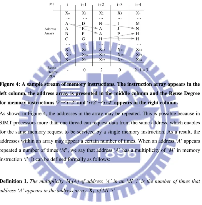
Figure 4: A sample stream of memory instructions. The instruction array appears in the left column, the address array is presented in the middle column and the Reuse Degree for memory instructions ‘i’ ‘i+2’ and ‘i+2’ ‘i+4’ appears in the right column.

As shown in Figure 4, the addresses in the array may be repeated. This is possible because in SIMT processors more than one thread can request data from the same address, which enables for the same memory request to be serviced by a single memory instruction. As a result, the addresses within an array may appear a certain number of times. When an address „A‟ appears repeated a number of times „M‟, we say that address „A‟ has a multiplicity of „M‟ in memory instruction „i‟. It can be defined formally as follows:

Definition 1. The multiplicity (A) of address ‘A’ in an MI ‘i’ is the number of times that address ‘A’ appears in the address array of MI ‘i’.

Once the concept of multiplicity has been defined, it is possible then to define the data reuse degree.

Definition 2. The data reuse degree (DS) between two MIs ‘i’ and ‘j’, where j>i, in an instruction stream is the sum of the multiplicities ( (t)) in MI ‘j’ for the array of addresses common to ‘i’ and ‘j’, given by:

14

∑

where , S is the size of the reference stream, | |, = {X0, X1, X2, … , XT} and Xk are memory addresses.

It is clear from Eq.1 that in order to determine it is first necessary to determine the

common address array , which holds the subset of addresses common to MI „j‟ common

to „i‟.

It is necessary to explain the previous definitions and metrics with concrete cases. In the example presented in Figure 4, it is possible to determine the reuse degree DS for some of the memory instructions in the sample instruction stream. In MI „i‟, address „A‟ appears twice, and it is used again in MI „i+2‟. In the latter, (A) = 2. Since „A‟ is the only address in the

common address array, then = {A} and . When analyzing the DS between

„i+2‟ and „i+4‟, we can see that the common address array is ={H, N}. The multiplicities

for addresses „H‟ and „N‟ in MI „i+4‟ are (H)=2 and (N)=1, respectively. Thus, the

reuse degree ∑ (H)+ (N) = 2+1 =3. The result

appears in the „Reuse Degree‟ column in Figure 4. Notice that the DS between MIs „i‟ to „i+1‟, „i+3‟ and „i+4‟ is zero (not undetermined). This is so because there are no common addresses between „i‟ and the other MIs different to „i+2‟. Similar conclusions can be drawn from the rest of MIs.

Once the reuse degree and associated metrics have been defined, it is then necessary to establish a formal relationship between the MIs in the instruction stream in order to obtain the data reuse characteristic.

4.1 Definition of the Reuse Distance

Proposing a definition of the reuse distance concept for SIMT machines becomes necessary in order to model the reuse characteristic of applications. We first examine the concepts behind the reuse distance as it is applied in more conventional processors, and subsequently formulate a definition for SIMT processors.

15

4.1.1 Traditional reuse distance analyses

When applying the reuse distance analysis for applications in uniprocessor and CMP systems, the concept of reuse distance is equivalent to the concept of stack distance using LRU (Least Recently Used) replacement policy as defined by Mattson [15]. In uniprocessor systems, only one data structure (stack, splay tree, among others) is used [16] to store the addresses that the program accesses during execution. Figure 5 illustrates the details of this methodology. In Figure 5(a), we can see a sample reference stream in a uniprocessor system. As previously mentioned, there is a one-to-one correspondence between the MI and the addresses referenced. Figure 5(b) shows a data structure, a stack in this case, changing state as data is requested. Whenever a memory access is issued by the processor, the stack is traversed to assess whether if the current address being accessed has been previously accessed. If so, as in MI „i+2‟ the RD for this address will be recorded as the number of different addresses i.e. number of entries, between the address being accessed and its previous entry. The previous entry is erased and the new entry is placed at the top of the stack, with an associated distance value. In case no previous entry for that address is found, the RD is recorded as infinity, as in MI „i‟.

Dist. = 1

i i+1 i+2 i+3 i+4 i+5 A B A A C B Dist. = 2 Addr. Dist. A ∞ Addr. Dist. B ∞ A ∞ Addr. Dist. A 1 B ∞ Addr. Dist. C ∞ A 1 B ∞ Addr. Dist. B 2 C ∞ A 1 B ∞ a) Addr. Dist. A 1 B ∞ A ∞ b)

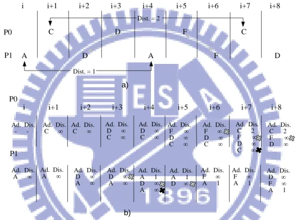
Figure 5: Reuse distance analysis as applied in uniprocessor systems. (a) Sample memory trace. (b) Changes of the state of the stack as memory instructions are issued. Additional considerations become necessary when applying the reuse distance analysis for CMP systems. Figure 6(a) presents a sample instruction stream for a CMP with separate memory subsystems. There are two processors, P0 and P1, that can request data simultaneously to their respective memories. We alternate the accesses by P0 and P1 for

16

simplicity, but it is not a necessary condition for this case. The one-to-one correspondence between the MI and addresses referenced is maintained from the stack‟s perspective. Additional details of the CMP system implementation are taken into consideration in order to model locality accurately [11]. Factors such as the presence of private memory subsystems and the details of the coherence mechanism become a part of analytical model for the reuse distance in CMPs.

i i+1 i+2 i+3 i+4 i+5 i+6 i+7 i+8

P1 A D A F D Dist. = 1 Ad. Dis. -Ad. Dis. C ∞ a) Ad. Dis. C ∞ b) P0 C D F C Ad. Dis. A ∞ P0 P1 Dist. = 2 Ad. Dis. D ∞ C ∞ Ad. Dis. D ∞ C ∞ Ad. Dis. F ∞ D ∞ C ∞ Ad. Dis. F ∞ D ∞ C ∞ Ad. Dis. C 2 F ∞ D ∞ C ∞ Ad. Dis. C 2 F ∞ D ∞ Ad. Dis. A ∞ Ad. Dis. D ∞ A ∞ Ad. Dis. D ∞ A ∞ Ad. Dis. A 1 D ∞ A ∞ Ad. Dis. A 1 D ∞ Ad. Dis. F ∞ A 1 Ad. Dis. F ∞ A 1 Ad. Dis. D ∞ F ∞ A 1

i i+1 i+2 i+3 i+4 i+5 i+6 i+7 i+8

Figure 6: Reuse distance analysis in CMP systems with private memory subsystem. (a) Sample reference stream. (b) Stacks for the private memory subsystem.

In Figure 6(b), we show the corresponding stacks for each memory subsystem in a system with two private memories, assuming that all references are store operations for illustrative purposes. In MI „i‟, processor P1 accesses address „A‟. This address is stored as the first entry in the stack of P1. In MI „i+3‟, processor P0 references address „D‟. This causes the invalidation of address „D‟ in the stack of P1, as illustrated by the gray cross at one side of the entry for „D‟ in „i+3‟. Despite being invalidated, it is maintained until it propagates to the bottom of the stack, as shown in MIs „i+3‟, „i+4‟ and „i+5‟. The entry is kept so not to alter the RD values that result from referencing another memory element that was referenced prior