位元率-失真度最佳化網路影像串流技術─可調變式編碼多點傳播

全文

(1)國立交通大學網路工程研究所碩士論文. 位元率-失真度最佳化網路影像串流技術 ─ 可調變式編碼多點傳播 Rate-Distortion Optimized Video Streaming Based Upon SVC Multicasting. 研究生：林哲民指導教授：邵家健. 中華民國. 教授. 九十七. 年九月.

(2) 位元率-失真度最佳化網路影像串流技術─可調變式編碼多點傳播 Rate-Distortion Optimized Video Streaming Based Upon SVC Multicasting. 研究生：林哲民. Student：Che-Min Lin. 指導教授：邵家健. Advisor：John Kar-kin Zao. 國立交通大學網路工程研究所碩士論文. A Thesis Submitted to Institute of Network Engineering College of Computer Science National Chiao Tung University in partial Fulfillment of the Requirements for the Degree of Master in. Computer Science September 2008 Hsinchu, Taiwan, Republic of China. 中華民國九十七年九月.

(3) 位元率-失真度最佳化網路影像串流技術─可調變式編碼多點傳播. 學生：林哲民. 指導教授：邵家健. 國立交通大學網路工程研究所碩士班. 摘. 要. 我們的目的是在於建立一套傳輸技術，用於可調變式編碼的多點傳播，如何做到這般的傳輸是個有趣而複雜的問題，由於這樣的編碼方式會分成較多層次，目的是要使的在不同使用者裝置之間可重複利用的部分增加，使的傳輸上更有效率。並且在目前的多媒體傳輸的網路架構之下，大部分的運用是在無線網路之上，並且有在同個區域網路下裝置同質性較高的特性，本篇論文便是利用編碼的特性和網路的架構來設計傳輸機制。. 我們提出了三個傳輸技巧使的網路傳輸更有效率，並且訂定簡化目標，依此建立一套訊息交換機制來協助網路節點做出決定，再提出了四種考慮不同因素的演算法架構來分配多媒體串流，最後建立一個模擬整個架構的程式來跑各種不同網路設定的實驗。. 從整個實驗的結果上可以觀察到以下幾項，第一是做到對於使用者裝置上都能獲得較好的播放品質，第二是在整個架構傳輸的網路頻寬使用上是有效率的，第三是使的網路上的串流集中，最後是可以發現到整個網路上的多媒體中繼節點的頻寬的使用上也是有效率的。. i.

(4) Rate-Distortion Optimized Video Streaming Based Upon SVC Multicasting Student: Che-Min Lin. Advisor: John Kar-kin Zao. Institute of Network Engineering National Chiao Tung University. ABSTRACT In this thesis, a video streaming scheme for conducting SVC multicasting is proposed. Scalable Video Coding consists of multiple layers and there is no redundancy between layers. We aim at such characteristics of SVC to design the video streaming scheme. The proposed scheme employs a combination of three transport techniques. We also define an optimization model and build a message exchange mechanism based on it. We set up four decision ordering algorithms to allocate video streams in the network. Finally, we implement a simulation for running our scheme under different settings. We can observe four results in our experiments: (1) better playback quality, (2) efficient bandwidth consumption in the network, (3) bitstream aggregation in the network, and (4) well-performed bandwidth usage of media gateways.. ii.

(5) 誌. 謝. 首先我最要感謝邵家健老師，這篇論文的題目、方向以及方法，都是經由跟老師不斷的討論、琢磨出來的，期間老師一直給我很多的指導、建議與修正才順利的完成這篇論文，若沒有老師辛勤的指導，我將不能獨力完成此篇論文；另外感謝老師這兩年對我的教導與栽培，無論是學術上研究能力與思考能力的諄諄善誘，或甚至是待人處事上一些教誨與經驗分享，實在使我獲益良多。感謝這段時間以來一起為畢業打拼的夥伴郭芳伯，在與他互相勉勵互相討論論文研究中，獲得了許多寫論文的感想與技巧；另外感謝胡嘉錡學弟幫忙我分攤完成許多實驗的模擬和數據的建立與分析，使我能夠專心的完成我的論文；感謝黃國晉學長在過程中不斷的與我相談一些研究上該注意的細節與不斷給我建議，讓我做一些技術上的諮詢，以及對於一些事物上的經驗分享；感謝楊鈞凱學弟以及大二的劉皓偉、李翰、以及李文平學弟幫我整理一些圖檔，使我不至於花費太多在人工操作上；感謝郭宇軒學長最開始的一些指導以及教導我使用模擬軟體 OMNeT++的技巧；最後感謝工三 620 實驗室曾一起努力過所有成員，包括了張哲維、朱書玄、李明龍、黃凌軒、劉育志學長，曾輔國同學，以及陳星閔、邱博政、王梅瑛、李勝焜、蘇彥霖、楊馥戍學弟妹們。. 最後我要感謝我的家人們，辛苦栽培我念書到現在研究所要畢業了，在我最困難的時候一直支持我，在我遇到瓶頸時給我鼓勵與意見，心中有萬千的感激，這篇論文是因為他們而產生的。還要感謝褘涵，謝謝她給予我十分多心靈上的支持與鼓勵，在我盪到谷底的時候始終在我旁邊陪著我度過。. 這篇論文需要感謝的人太多了，謝謝你(妳)們。 iii.

(6) Contents Chapter 1 . Introduction ................................................................................. 1 . 1.1 . Problem Statement ........................................................................................... 1 . 1.2 . Research Approach........................................................................................... 3 . 1.3 . Thesis Outline ................................................................................................... 4 . Chapter 2 . Related Work ............................................................................... 5 . 2.1 . SVC Inter-layer Dependencies and Rate-Distortion Performance .............. 5 . 2.2 . Bandwidth Efficiency of Internet Video Streaming using AVC vs. SVC ..... 6 . 2.3 . Early Attempt of Peer-to-Peer SVC Streaming ............................................. 7 . Chapter 3 . Techniques.................................................................................... 9 . 3.1 . Network Topology ........................................................................................... 10 . 3.2 . Broadcasting over Stub Networks ................................................................. 11 . 3.3 . En-route Bitstream Aggregation ................................................................... 12 . 3.4 . Information Dispersal and Multipath Transport ........................................ 13 . Chapter 4 . Algorithms ................................................................................. 15 . 4.1 . Optimization Model........................................................................................ 15 . 4.2 . Bandwidth Allocation Algorithm .................................................................. 16 4.2.1 . Provider-Subscriber Negotiation for Bandwidth Allocation .................... 17 . 4.2.2 . Ordering of Bandwidth Allocation Negotiations ...................................... 18 . 4.2.2.1 . Algorithm 1: Ordering without Consideration of Device Distribution ........18 . 4.2.2.2 . Algorithm 2: Ordering with Consideration of Global Device Distribution .20 . 4.2.2.3 . Algorithm 3: Ordering with Local Fair Competition ...................................21 . 4.2.2.4 . Algorithm 4: Local Ordering with Local Dominated Request ....................22 . 4.2.2.5 . Examples of four algorithms........................................................................23 . Chapter 5 5.1 . Message Exchange..................................................................... 25 Message Exchange Mechanism ..................................................................... 25 . Chapter 6 . Experiments ............................................................................... 29 . 6.1 . Platform ........................................................................................................... 29 . 6.2 . Models .............................................................................................................. 30 6.2.1 . Network Model ......................................................................................... 30 . 6.2.2 . Source Model............................................................................................ 32 . Chapter 7 . Results and Analysis.................................................................. 33 . 7.1 . PSNR Reduction ............................................................................................. 34 . 7.2 . Normalized PSNR Reduction ........................................................................ 37 iv.

(7) 7.3 . SVC vs. AVC .................................................................................................... 39 . 7.4 . Efficiency ......................................................................................................... 40 . 7.5 . Layer Bandwidth Ratio .................................................................................. 41 . 7.6 . Average Media Gateway Bandwidth Usage ................................................. 43 . Chapter 8 . Conclusion .................................................................................. 46 . 8.1 . Accomplishment ............................................................................................. 46 . 8.2 . Future Work .................................................................................................... 47 . Glossary References. 48 49 . v.

(8) Figures. Figure 1: Heterogeneous SVC Multicasting Architecture .......................................................... 9 Figure 2: Subscribers and Providers ......................................................................................... 11 Figure 3: Aggregation of data flows ......................................................................................... 12 Figure 4: Negotiation for a Layer Set on a link between Subscriber and Provider .................. 17 Figure 5: Message Exchange Mechanism ................................................................................ 26 Figure 6: Graphic User Interface of Simulation for Bandwidth Reservation Protocol ............ 29 Figure 7: Network Model ......................................................................................................... 30 Figure 8: Dependency Relationship ......................................................................................... 32 Figure 9: PSNR Reduction ....................................................................................................... 35 Figure 10: PSNR Reduction of Algorithm 1 ............................................................................ 36 Figure 11: PSNR Reduction of Algorithm 2 ............................................................................ 36 Figure 12: PSNR Reduction of Algorithm 3 ............................................................................ 36 Figure 13: PSNR Reduction of Algorithm 4 ............................................................................ 37 Figure 14: Normalized PSNR Reduction ................................................................................. 37 Figure 15: Normalized PSNR Reduction of Algorithm 1 ........................................................ 38 Figure 16: Normalized PSNR Reduction of Algorithm 2 ........................................................ 38 Figure 17: Normalized PSNR Reduction of Algorithm 3 ........................................................ 38 Figure 18: Normalized PSNR Reduction of Algorithm 4 ........................................................ 39 Figure 19: Difference between SVC and AVC of four algorithms ........................................... 40 Figure 20: Efficiency for four algorithms................................................................................. 41 Figure 21: Layer Bandwidth Ratio of Algorithm 1 .................................................................. 42 Figure 22: Layer Bandwidth Ratio of Algorithm 2 .................................................................. 42 Figure 23: Layer Bandwidth Ratio of Algorithm 3 .................................................................. 43 Figure 24: Layer Bandwidth Ratio of Algorithm 4 .................................................................. 43 Figure 25: Average Media Gateway Bandwidth Usage of algorithms ..................................... 44 Figure 26: Average Media Gateway Bandwidth Usage of Algorithm 1 ................................... 44 Figure 27: Average Media Gateway Bandwidth Usage of Algorithm 2 ................................... 45 Figure 28: Average Media Gateway Bandwidth Usage of Algorithm 3 ................................... 45 Figure 29: Average Media Gateway Bandwidth Usage of Algorithm 4 ................................... 45 . vi.

(9) Tables. Table 1: Pseudo Code of Ordering Algorithm in Algorithm 1 and 2 ........................................ 19 Table 2: Pseudo Code of Function Rate_Distortion_Gain(LAYER) in Algorithm 1 ............... 19 Table 3: Pseudo Code of Function Rate_Distortion_Gain(LAYER) in Algorithm 2 ............... 21 Table 4: Pseudo Code of Algorithm 3 ...................................................................................... 22 Table 5: Pseudo Code of Algorithm 4 ...................................................................................... 23 Table 6: Characteristics of SVC test bitstream......................................................................... 32 Table 7: Original Layer Counts and Layers Counts in lower tiers ........................................... 42 . vii.

(10) Chapter 1. 1.1. Introduction. Problem Statement. The Scalable Video Coding (SVC) Extension of H.264/AVC [1] specifies a multilayer predictive encoding scheme that enables different video coding layers to be extracted and decoded selectively by different user devices according to their playback capability and transport network throughput. This desirable property causes SVC to be regarded as the ideal technology for providing multimedia multicasting to heterogeneous viewing devices. Nevertheless, a close examination of SVC data format reveals two potential handicaps of its use in heterogeneous multicasting. First, the cumulative bit rates of the SVC layers extracted by individual user devices routinely exceed the bit rates of their corresponding AVC bitstreams due to the loss of coding efficiency in multilayer encoding. When the SVC bitstreams are transported over bandwidth stringent networks such as the cellular telephone networks, this bit rate inflation often implies cost inflation or performance degradation. Second, the inter-layer dependence relations introduced by the multilayer predictive encoding process requires a viewing device to extract and decode all the reference coding layers on which the target layer of the device depends before the device can decode its target layer. Any un-recoverable loss of a reference layer will reduce the decodable layers to those below the lost layer due to inter-layer dependency and thus degrade the playback quality on the viewing devices. In a best-effort delivery network such as the Internet, a congested along a transport rate can thus a degradation of the video playback quality. Thus, a bandwidth efficient and loss. 1.

(11) resilient transport scheme must be devised in order to ensure SVC to be the preferred encoding format for video streaming. In this thesis, we attempted to improve the bandwidth efficiency of heterogeneous multicasting of SVC bitstreams by devising a distributed bandwidth allocation scheme that can be implemented by every intermediate node along the transport paths. The objective of our scheme is to maximize the overall video playback quality of the viewing devices enrolled in the heterogeneous multicasting session while minimizing the total bandwidth utilization along the transport paths. Our bandwidth allocation scheme assumes that the SVC bitstream is transported to different types of viewing devices scattered across multiple stub networks over the Internet via several multicast trees each of which is made up of tiers of intermediate nodes (known as the media gateways). Every media gateway (MG) receives specific SVC layers from a finite set of upstream nodes along multiple inbound network connections and dispatches these layers to specific downstream nodes through multiple outbound network connections. Each MG decides how to allocate its outbound bandwidth for transporting specific SVC layers to specific downstream nodes based only on the local information it gathers from its upstream and downstream nodes. No information exchange among the media gateways in the same tier is allowed. To simplify the preliminary design of our scheme, we ignore the asynchronous and lossy nature of the transport network with respect to information exchanges regarding bandwidth allocation. Hence, the decisions of individual MGs are unaffected by the order and the potential loss of control packets.. 2.

(12) 1.2. Research Approach. We will first introduce transport techniques for efficient purpose of SVC multicasting. ¾. Broadcasting over stub networks is to compensate the bit rate inflation introduced by SVC multilayer encoding process.. ¾. En-route Bitstream Aggregation over long haul network is to minimize upstream bandwidth while maximize serviced device numbers.. ¾. Information Dispersal and Multipath Diversity is to cut layers into equal-rated flows to fit into media gateway more easily and to add error protections on layers unequally by their importance shown in the inter-layer dependency.. There are a lot of different video streams in the network and to we will arrange bitstream allocation of them in a bandwidth efficient and loss resilient transport under these three techniques. Then we will formulate our goal in an optimization models about both playback quality and network bandwidth consumption. And we will design algorithms under this model. There are some considerations of SVC we should introduce. Both theoretic and empirical work point to some important factors that are highly relative to the performance of bandwidth allocation of the SVC multicasting as the followings: ¾. Inter-layer Dependency: To avoid wastes of bandwidth, viewing devices must not subscribe to any layer that can’t be decoded. On the other hand, they will make subscription based on the extraction path of SVC.. ¾. Bitstream Characteristics: SVC layers have their own bandwidth consumption and improvement of playback quality. The Rate Distortion Ratio of a single SVC layer. 3.

(13) influences the efficiency of transporting it directly. ¾. User Device Types and Distribution over the Internet: Since we want to arrange the bandwidth allocation among large amount of devices, user device types and their distribution should be considered carefully. The largest amount of viewing devices will dominate the performance of bandwidth allocation.. ¾. Network Topology: Since we want to arrange the bandwidth allocation over large scale networks, to make a better bandwidth allocation under a specific sub-network highly depends on its topology.. We will consider these factors and design different decision algorithms to approach our goal.. 1.3. Thesis Outline. In chapter 2, we will briefly introduce the related work of SVC multicasting. In chapter 3, we will introduce efficient transport techniques. In chapter 4, we describe the optimization model and decision algorithms for bandwidth allocation. In chapter 5, we will explain our message exchange mechanism in detail. In chapter 6, we will show how we implement the scheme and the how we design the experiment models. In chapter 7, we will define the measurements and give the results and its analysis. In chapter 8, we will make a conclusion and tell accomplishments in our works and our future works. And the end of paper, we add a glossary about definitions of symbols we used in this thesis.. 4.

(14) Chapter 2. 2.1. Related Work. SVC Inter-layer Dependencies and Rate-Distortion Per-. formance. In [2], it is an overview of Scalable Video Coding Extension of H.264/AVC Standard. Scalable Video Coding (SVC) provides scalabilities refers to the removal of parts of the video bitstream in order to adapt it to the various needs or preferences of end users as well as to varying terminal capabilities or network conditions. It has three modes about temporal, spatial, and quality scalability. Spatial scalability and temporal scalability represent the picture size (spatial resolution) or frame rate (temporal resolution). With quality scalability, the bitstream provides the same spatial and temporal resolution, but with a lower fidelity which is often referred to as signal-to-noise ratio (SNR Scalability). For different scalabilities, viewing devices can easily choose layers based on device capabilities and subscribe layers according to extraction path from base layer to enhancement layers. Hence, they may receive fewer layers if congestion occurs. Scalable Video Coding encodes a video clips into a base layer and many enhancement layers with different resolutions. To receive layers following different extraction paths will get decodable video clips with the same content but in different resolutions. Every extraction path starts from the same layer which is called the Base Layer. Every viewing device could. 5.

(15) improve its playback quality by receiving more enhancement layers. Each layer has different improvement of playback quality and different bit rate. The measurement of distortion we used is called Peak Signal to Noise Ratio (PSNR). These characteristics of different layers effect the decisions of serving nodes in the network.. 2.2. Bandwidth Efficiency of Internet Video Streaming using. AVC vs. SVC. In [3], Kim compared three approaches for video multicasting as following: z. The replicated stream approach [4], [5] In this approach, source is encoded into multiple independent video streams with different bit-rates because of different compression parameters. And then these streams will be multicast over the network to all viewing devices. AVC Simulcasting is similar to this approach.. z. The cumulative layering approach [6], [7] In this approach, source in encoded into one base layer and multiple enhancement layers. Base layer can be decoded independently but enhancement layers should be decoded cumulatively. Devices improve their playback quality by receiving more enhancement layers. SVC Multicasting is this kind of approach.. z. The non-cumulative layering approach [8], [9]. 6.

(16) In this approach, source in encoded into multiple independent layers. All layers can be decoded independently and devices improve their playback quality by receiving more layers. As we referred, the first one is like the AVC Simulcasting and the second one is the SVC Multicasting. He considered and estimated different overheads of layered video such as packetization overhead, protocol overhead, and error control overhead. Then he gave basic Rate Allocation and Stream Assignment algorithms for three different approaches for simulations. He simulated three approaches and analyzed with four measurement average reception rate, average effective reception rate, total bandwidth usage, and efficiency. He got conclusions that the performance of heterogeneous video multicasting schemes depend on the amount of layering overhead and said that if the effective reception rate is the same, replicated stream multicasting is preferred except receivers are clustered in few domains. However, if we use unicast in the local subnet, SVC layers are redundantly transported and the independency of SVC layers has not been used. Hence, we should broadcast layers in the local subnet to avoid transport of redundant layers. Furthermore, the question of SVC multicasting is not WHETHER SVC is efficient. It is HOW to transport SVC in a efficient way with using its merits and to compensate its shortcomings.. 2.3. Early Attempt of Peer-to-Peer SVC Streaming. In [10], Baccichet et. al. proposed a combined use of tree-based push transport and en-route progressive rate adaptation of SVC bitstreams to achieve low-latency peer-to-peer video streaming. By enabling the intermediate relaying nodes to extract the SVC layers demanded by. 7.

(17) their down-stream peers, the proposed scheme reduces the chance of link congestion. Moreover, by forwarding the IP packets carrying an SVC bitstream along several multicast trees, the scheme is expected to amortize the impact of individual packet loss and link failure. Baccichet’s scheme can indeed eliminate the need for layer synchronization and thus reduce SVC transport latency by pushing the multi-layer bitstream through several multicast trees. However, its effectiveness in removing link congestions is somewhat dubious because en-route SVC rate adaptation can only work when same types of user devices are gathered in clusters over the multicast network, which is the case we refer to as homogeneous clustering. If different types of devices are dispersed over the network as in the case of heterogeneous clustering then the relaying nodes have no choice but to forward almost the entire SVC bitstream to the downstream peers. Besides, the usefulness of IP packet dispersal (without the employment of erasure protection) is also questionable because most SVC NAL units are likely carried in multiple IP packets. The loss of any of these packets will render the entire NAL unit undecodable. As a result, Baccichet’s scheme performs well only under low traffic load and mild packet loss.. 8.

(18) Ch hapteer 3. Tech hniqu ues. The proposed p heterogeneouus SVC muulticasting sccheme was based uponn the idea of o multipathh transsport of incrremental SV VC NAL setss (abbreviated hereafterr as SVC-IN NS or simply y INS). Thee schem me employss a combinaation of threee transportt techniquess: (1) broadccasting of SVC-INS S inn locall service subbnets, (2) agggregation of o data flows along their transport ppaths and (3 3) multipathh transsportation of SVC-INS over long--haul netwo orks. This multicasting m scheme is particularly p y suiteed for delivvering SVC C bitstream ms to different types of user ddevices scatttered overr geoggraphically dispersed local l subneets. [Figure 1] illustraates a typiccal deploym ment of thee schem me over muultiple wirelless networkks that span n across the Internet.. Figure 1: Heterogenneous SVC Multicastinng Architectture Like Baccichet’s scheme, our schem me relies on n intermediiate nodes, known as the mediaa gatew ways (MGs), to shape transport trraffic. Insteead of havinng the relayying nodes performingg. 9.

(19) bitstream extraction and rate adaptation, our scheme requires its MRs to perform the following operations: (1) broadcast the SVC-INS received from their upstream nodes to the user devices present in their local service subsets; (2) request the SVC-INS needed by their downstream nodes from their upstream nodes while trying to minimize the number of data flows between these nodes; (3) disperse the data flows carrying the same SVC-INS among different MRs in order to balance the traffic load and use unequal erasure protection (UEP) in order to protect data flows carrying different SVC-INS. Our scheme can be adapted to both content-delivery and peer-to-peer architectures. When it is deployed on top of a content-delivery architecture such as HP MSM-CDM [11], the media relays (MRs) shall be deployed at each service subnets as well as strategic points-of-presence (PoPs) in order to maximize the benefit of flow aggregation and load balancing. When the scheme is used in a peer-to-peer application, some of the more capable peer nodes will select to play the role of MRs and perform the required operations. The peer-to-peer application can use any multiple tree push architecture including Stanford Peer-to-Peer Multicast (SPPM) protocol [1], Split-Stream [12] or Trickle [13] to establish the multicast mesh. In both cases, the MRs shall be deployed at the edge of the Internet in the user service subnets or the ISP stub networks that are connected to the Internet backbone.. 3.1. Network Topology. For the heterogeneous SVC multicast architecture in [Figure 1], we make an assumption for a network model in this thesis. For a video source and many viewing devices which will subscribe to the video, there are many other intermediate nodes in the network called Media Gateways (MGs) for relaying video to viewing devices. We assume that there are three tiers in 10.

(20) the network, n thaat is, tier 0, 1, and 2 from f bottom m to top annd MGs in the same tiier may nott exchhange inform mation withh each othher. MGs in n the tier 0 serve vieewing devicces in stubb netw work and facce to requeests from devices direcctly. MGs in i the tier 1 located in upstream m aggreegation ISP Ps is as the backbone of o the network. MGs in i the tier 2 are adjaceent to videoo sourcce and helpp the videoo source multicast m SV VC layers. Our techniiques, algorrithms, andd mechhanisms aree based on thhis networkk model from m the bottom m to the topp.. Figure 2: Subscriberrs and Proviiders Sincee we use a network assumptionn about tierrs, we call them provviders and subscriberss betw ween two tieers as in [Fiigure 2]. A subscriber or a providder is able to connect to multiplee proviiders or subbscribers. The T providerr will determ mine what layer will bbe served on n what linkk and allocate a its bandwidth to the subsscription, an nd the subsscriber will make decissions aboutt sendiing subscripption to whiich providerr.. 3.2. Broaadcastin ng over Stub S Netw works. The first bandw width savinng techniquue we emp ployed was the simplee broadcastting of thee C-INS in dem mand over thhe local servvice subnetss to the userr devices coonnected to the t subnets.. SVC Eachh SVC-INS should be transmittedd over separate broaddcast channnel and prottected withh. 11.

(21) forw ward error coorrection (FE EC) at the physical p lay yer. This brooadcasting m mechanism can c be usedd not only o over wiireless and cellular c netw works but can also be used u in mostt local accesss networkss incluuding wiredd Ethernet, cable televvision netw works and ADSL A as thhey are alll inherentlyy broaddcasting nettworks. If an SVC bitstreeam is subsccribed by many m user deevices in thee same subnnet then broaadcasting off SVC C-INS eliminnates the neeed to send multiple co opies of the same bitstrream over the t networkk and thus t incur significant s r reduction off bandwidth h usage. Thhis saving iss more than n enough too comppensate the bit rate inflaation introduuced by thee SVC multilayer encodding processs. If an SVC C bitstrream has few w subscribeers in a locall subnet then n it should be b convertedd to H.264 AVC A formatt throuugh SVC-too-AVC bitstrream rewritting [14].. 3.3. En-rroute Bittstream Aggrega ation. Figure 3: Aggregatio on of data flows fl 12.

(22) Another bandwidth saving technique is the aggregation of data flows [Figure 3] along their transport routes. In an SVC multicast, many user devices will require the same set of layer in order to playback the video. The media gateways (MGs) embedded in the multicast trees can function as aggregation points of these data flows. We designed a bandwidth reservation protocol to implement the en-route aggregation of data flows. The protocol adopted a bottom-up approach in conducting bandwidth negotiations among two tiers of MGs like a 4-way handshake protocol. Between the two tiers, the nodes in the lower tier are called subscribers, and the upper nodes are called providers. Subscribers know the layer it needs and the providers it can access in the upper tier. The purpose of the negotiation is to enable the subscriber to choose a provider for each layer or derived data flow. To do so, the subscriber keeps a matrix of serving probability information of the accessible providers, and makes decisions based on the probability information. Providers should also make decisions on whether to accept or refuse the requests submitted by the subscribers. Every provider publishes a probability list of layers it intends to transport.. 3.4. Information Dispersal and Multipath Transport. In order to ensure that different SVC-INS can be delivered to the user devices that need them even amidst significant traffic load and packet loss, our scheme employs the communication techniques of multipath diversity (MD) and unequal erasure protection (UEP) to protect the transport of individual INS. Such a protection is particularly important for those INS that are extracted from the lower SVC layers as they are the ones on which the upper SVC layers are depended for motion and residual prediction. Under the protection, each SVC-INS is coded and divided into multiple equal-rated data flows by a spatial-temporal UEP encoder. Each of 13.

(23) these data flows is then dispersed into different transport routes in the multicast trees. To decode an INS, a user device or a media relay only need to collect sufficient amount of code words derived from the INS and submit them to a UEP decoder. The design of a spatial-temporal UEP encoder suitable for SVC transport is currently underway. Hence, the investigation of the effectiveness of this technique lies beyond the scope of this paper.. 14.

(24) Chapter 4. 4.1. Algorithms. Optimization Model. Although falling short of producing a formal proof, we postulate that the problem of bandwidth allocation for a SVC multicasting session that maximizing device playback quality while minimizes total bandwidth consumption is a NP-Hard problem. Hence, a distributed bandwidth allocation algorithm must rely on iterative heuristics to search for the optimal solution. In this chapter, we propose an iterative negotiation between providers and subscribers and four different algorithms to arrange these negotiations that aim at directing the iterative negotiation towards an optimal solution. We want to maximize the playback quality of viewing devices but we also hope to transport SVC layers in a bandwidth efficient network. Hence, we define the “Rate-Distortion Gain (R-D Gain)” function as (1). The numerator is the PSNR Improvement that is the playback quality gain of a device from receiving a specific layer and the denominator means that the bandwidth consumption of the layer in the network. For every received layer in every viewing device, we divide the PSNR improvement by the cumulative bandwidth consumption of the transport path of such layer. We assume that the transport path of Layer L in D bottom to top is D. , MG 0,. , MG 1,. serving devices counts of device type U MG ,. , … , MG T,. ,. represents the. in the transport sub-tree which has the root. . Then we calculate the R-D Gain of Layer L in D. distortion gain of D. and nU. from. where d D. , L means the. receiving L and the first term in the denominator means the copies of 15.

(25) L. L in the local subnet. The value is 1 if unicast, and U. ,L. U. ,. if broadcast in the. local subnet.. γ D. d D. ,L. U. 4.2. Σ,L. T. r L. nU. 0,. ,L. 1. 1. Σ 0. U. Σ,L. r L. nU. ,. Bandwidth Allocation Algorithm. The basic principle of our scheme is that viewing devices will not send subscription requests for layers that can not be decoded. That is, the bottom-up scheme will repeat many rounds and all viewing devices send requests for one or more decodable layers at once based on the dependency of layers. We’ll first introduce the negotiation between providers and subscribers. This will show us how every provider and every subscriber negotiates bandwidth allocation of a layer on a network link. Then we design four different sequencing algorithms that differ from considering factors increasingly, as we have referred to, bitstream characteristics, device type population distribution, and network topology. These algorithms will determine whole network or local viewing devices make requests of layers in what kind of order.. 16.

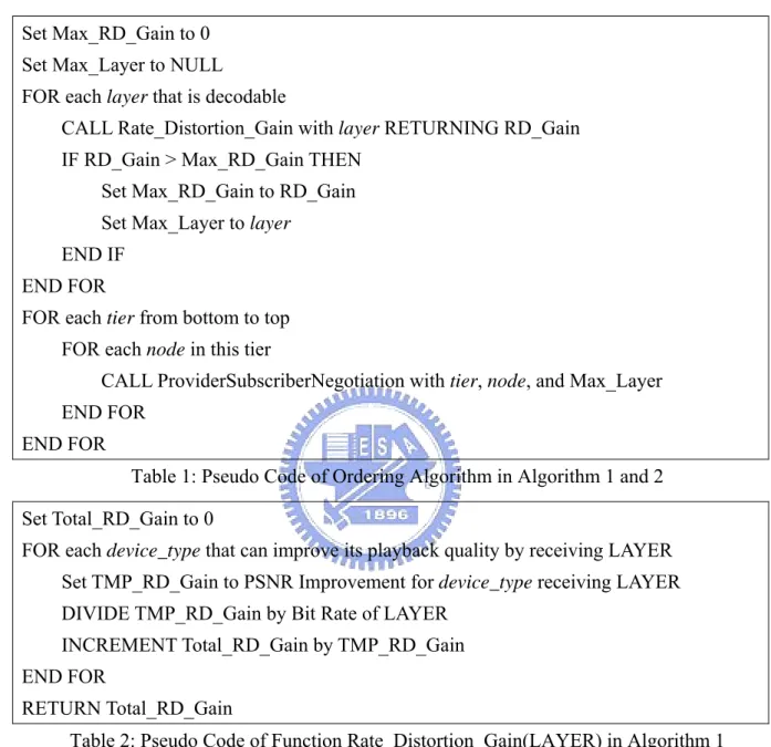
(26) 4.2.1. Provvider-Sub bscriber Negotiat N ion for Bandwidt B th Alloca ation. Figure 4:: Negotiatioon for a Layyer Set on a link betweeen Subscriber and Prov vider This negotiationn is to deterrmine a specific layer set s of layerss transporteed on a speccific link inn the network n beetween provviders and subscriberss as in [Fiigure 4]. T The provideer will firstt comppute the exppectation vaalue about layers that could c be alloocated from m it for each h subscriberr as (22). The firstt term is alllowed layerr counts forr the providder MG term means the importancee of MG ,. 1,. and the secondd. where importance i is computeed by ratio of o expectedd. R-D Gain of a specific s subbscriber amoong all subsscribers. Thhen the subsscriber will choose thee proviider which has largest expectationn to serve it as (3). At last, l provideers will cum mulate thesee requeests and coompare the expectatioon value off R-D Gainn of acceptting each request r andd alloccate the banndwidth from m the biggeest one. The expected R-D Gain is computeed as (4) byy subsccribers and sent to providers. It means m that how h much R-D R Gain anny providerr could earnn if it accepts a thiss request. R-D R Gain is total PSNR R Improvem ment of deviices divided d by bit ratee of that layer andd then divided by the acccessible prrovider counnts ξ , .. 17.

(27) E. 1, ; , ; L. LayerCount A. γ , ,L. 1, , L G. Σ ,. ,. γ , ,L. , 2. 1. γ , ,L. MG. γ , ,L. ,. ξ. 1, ̂. ̂. 1 ξ. Σ U ,L. ,. nU. ,. | max E. Σ U ,L. nU. d U. ,L. r L 1, ; , ; L. ,. d U. 3. ,L. r L. 4. 4.2.2 Ordering of Bandwidth Allocation Negotiations 4.2.2.1 Algorithm 1: Ordering without Consideration of Device Distri. bution . In this ordering of bandwidth allocation negotiations, we allocate the necessary bandwidth to transport SVC layers one at a time from the base layer to the highest enhancement layers according to their inter-layer dependency relationship and rate-distortion information. The numbers of rounds will be as same as the amount of layers. The Ordering Algorithm is as [Table 1]. The order is according to the dependency and if there is more than one decodable layer, we will choose a layer based on its rate distortion information. Hence, we will compare their Rate Distortion gain for such layer, which is the sum of PSNR improvement for all device types that can play this layer divided by its bit rate as [Table 2]. The advantage of this way is that the order of the resource reservation could be determined right after encoding, and it performs well when the population distribution makes no 18.

(28) difference since it is not sensitive to the population distribution. The performance will be bad if the population distribution is biased. Set Max_RD_Gain to 0 Set Max_Layer to NULL FOR each layer that is decodable CALL Rate_Distortion_Gain with layer RETURNING RD_Gain IF RD_Gain > Max_RD_Gain THEN Set Max_RD_Gain to RD_Gain Set Max_Layer to layer END IF END FOR FOR each tier from bottom to top FOR each node in this tier CALL ProviderSubscriberNegotiation with tier, node, and Max_Layer END FOR END FOR Table 1: Pseudo Code of Ordering Algorithm in Algorithm 1 and 2 Set Total_RD_Gain to 0 FOR each device_type that can improve its playback quality by receiving LAYER Set TMP_RD_Gain to PSNR Improvement for device_type receiving LAYER DIVIDE TMP_RD_Gain by Bit Rate of LAYER INCREMENT Total_RD_Gain by TMP_RD_Gain END FOR RETURN Total_RD_Gain Table 2: Pseudo Code of Function Rate_Distortion_Gain(LAYER) in Algorithm 1. 19.

(29) 4.2.2.2 Algorithm 2: Ordering with Consideration of Global Device . Distribution . In this ordering of bandwidth allocation negotiations, we allocate the necessary bandwidth to transport SVC layers one at a time from the base layer to the highest enhancement layers according to their inter-layer dependency relationship and rate-distortion information, and furthermore, the global device population distribution is considered in this case. Times of execution rounds will be as same as the number of layers. The Global Ordering Algorithm is as [Table 1]. The order is according to the dependency and if there is more than one decodable layer, we will choose a layer based on its single layer rate-distortion characteristic and the population distribution of viewing devices. Hence, we will compare their R-D gain for types of viewing devices, which is the sum of PSNR improvement for all viewing devices that could play that layer divided by its bit rate as [Table 3]. MGs in the top of the mesh can get the device population information easily by aggregating from the bottom and then propagate the global order to the bottom. The advantage of this algorithm is that it is sensitive to the population distribution, so different distribution may have orders that fit in such situation. But media gateways and devices may need extra information besides a local network since this is a global view that the population information will be cumulated to the top and then propagate the determined order to the bottom devices.. 20.

(30) Set Total_RD_Gain to 0 FOR each device_type that can improve its playback quality by receiving LAYER Set TMP_RD_Gain to PSNR Improvement for device_type receiving LAYER MULTIPLY TMP_RD_Gain by population of device type DIVIDE TMP_RD_Gain by Bit Rate of LAYER INCREMENT Total_RD_Gain by TMP_RD_Gain END FOR RETURN Total_RD_Gain Table 3: Pseudo Code of Function Rate_Distortion_Gain(LAYER) in Algorithm 2. 4.2.2.3 Algorithm 3: Ordering with Local Fair Competition . In this ordering of bandwidth allocation negotiations, we allocate the necessary bandwidth to transport all decodable SVC layers at a time from the base layer to the highest enhancement layers according to their inter-layer dependency relationship, rate-distortion information, and the local device population distribution as in [Table 4]. So competitions between different layers exist in this ordering in sub-trees of MGs. Differ from algorithm 1 and 2, there will be more than one layer allocated in the network and the competition of requests for all decodable layers may occur. Different local population distributions and local network topology affect local bandwidth allocations. The advantage of this case is that not only population distribution is considered but also the network topology takes place in the decisions. This local information may make the bandwidth allocation perform better, but the length of extraction path will have large effect in this case.. 21.

(31) FOR each tier from bottom to top FOR each node in this tier FOR each layer that is decodable for devices or required by media gateways CALL ProviderSubscriberNegotiation with tier, node, and layer END FOR END FOR END FOR Table 4: Pseudo Code of Algorithm 3. 4.2.2.4 Algorithm 4: Local Ordering with Local Dominated Request . In this ordering of bandwidth allocation negotiations, we allocate the necessary bandwidth to transport one dominated SVC layer (which brings the largest R-D Gain in the sub-tree) at a time for one MG from the base layer to the highest enhancement layers according to their inter-layer dependency relationship, rate-distortion information, and the local device population distribution as in [Table 5]. There will be many requests for different layers competing in the network but there is a difference between Algorithm 3. That is, all decodable layers will be requested from a subnet but in this Algorithm 4 there will be only one request from a subnet which will bring the largest R-D Gain. The request which represents the largest R-D Gain in a subnet will beat other requests rather than accepting all decodable layers. The advantage is that a local network view of device distribution will make accurate requests and nodes will not need extra information of nodes in other subnets. The length of extraction path will have smaller effect than Algorithm 3.. 22.

(32) FOR each tier from bottom to top FOR each node in this tier FOR each layer that is decodable for devices or required by media gateways CALL ProviderSubscriberNegotiation1 with tier, node, and layer END FOR END FOR END FOR Table 5: Pseudo Code of Algorithm 4. 4.2.2.5 Examples of four algorithms . We assume that the video source have been encoded into four layers, base layer 0 and enhancement layer 1, 2, and 3. Layer 1 and 2 depend on layer 0 and layer 3 depend on layer 1. Suppose that the device population in whole network is as ||{0,3}|| > ||{0,1}|| > ||{0,2}|| > ||{0}||, but the order of Rate-Distortion Gain is as 0>1>2>3. For algorithm 1 and 2, there is only one layer allocated in the network. Allocated order in algorithm 1 is {0, 1, 2, 3} which is the same as the layer R-D characteristics but {0, 1, 3, 2} in algorithm 2 since the population affect the order directly. For algorithm 3, all decodable layers will be allocated in the network, so layer 0 that all devices need will be allocated first. Layer 1 and layer 2 will be the next because they both depend on layer 0 and layer 3 will be the last one since it has the longest extraction path. Algorithm 4 is quite different so we provide another example for it. Assume that there are two MGs A, B in the same tier and MG A has 1000 devices requesting for layer 1 in its sub-tree and 10 for layer 2 where MG B has 10 devices for layer 1 in its. 1. There is only one difference in it that Providers will provide only one layer which brings largest Rate. Distortion Gain for serving it in the sub-tree in the same round. Provider will only serve the dominated layer request in its subnet rather than all decodable layers.. 23.

(33) sub-tree and 1000 for layer 2. Suppose that layer 0 has already been allocated, so layer 1 and layer 2 are both decodable now. For algorithm 3 that all decodable layers will be allocated, layer 1 and 2 will be allocated both in MG A and B and layer 3 will be allocated in the next round. But for algorithm 4, only the dominated layer in the sub-tree will be allocated. That is, MG A will accept requests for layer 1 and postpone requests for layer 2 and MG B does the opposite. In the next round, MG A will consider layer 2 and 3 at the same time since layer 3 is decodable after layer 1 being allocated, and MG B can only allocate layer 1 because it is the only decodable layer.. 24.

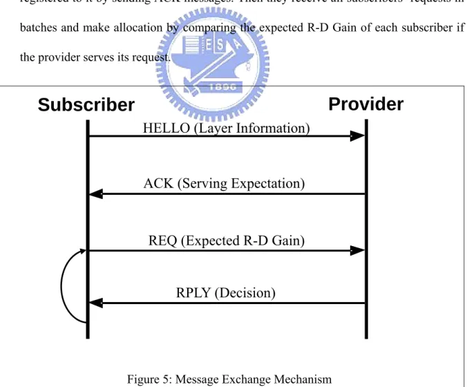
(34) Chapter 5. Message Exchange. A bandwidth saving technique we employed was the aggregation of data flows along their transport routes. In an SVC multicast, many user devices will require the same set of layers in order to playback the video. The media gateways (MGs) embedded in the multicast trees can function as aggregation points of these data flows. We designed a distributed bandwidth reservation message exchange mechanism to realize en-route aggregation of data flows. The mechanism is a multiple round bottom-up architecture conducted among two consecutive tiers of network nodes known as the subscribers and the providers. Each subscriber can negotiate with certain number of providers about the layer it needs and the number of user devices it serves. However, no communication between non-consecutive tiers is permitted nor communication among providers or subscribers in the same tier. The following section will show how we do the message exchange between subscribers and providers.. 5.1. Message Exchange Mechanism. The bandwidth allocation is initiated by user devices in the lowest tier and propagated towards the providers in the top tier. As in [Figure 5], subscribers register themselves to providers first about the served layer and layer set that refer served layer and the amount of devices that each layer is demanded by sending HELLO messages. The message is for providers to understand how many subscribers connect to it and their requirements and then 25.

(35) subscribers submit resource requests REQ messages that maximize probability of successful allocation and maximize aggregation of bitstream. Requests are submitted to chosen providers based on expectation value about layers that could be allocated by providers. They will choose one provider that has highest expectation values for served layer that they demand in each round. If the request failed, they will turn to the provider that has the highest expectation among the rests in next round. a). The provider receives registrations from subscribers and then derives serving probabilities for every subscriber by computing how many requests are allowed and subscribers’ importance for it, and then sends the probability to subscribers who registered to it by sending ACK messages. Then they receive all subscribers’ requests in batches and make allocation by comparing the expected R-D Gain of each subscriber if the provider serves its request.. Provider. Subscriber HELLO (Layer Information). ACK (Serving Expectation). REQ (Expected R-D Gain) RPLY (Decision). Figure 5: Message Exchange Mechanism. 26.

(36) The message exchange in the bandwidth allocation and their payloads are listed below: ¾ HELLO is shown in (5). It is sent by every subscriber MG ,. , which represents the. MG in tier . A HELLO message contains serving layer L , layer information tuples U. , nU. ,. U. ,L. which contains device types (U. number of a specific device type(nU accessible provider counts ξ ,. .. HELLO ,. ,. L, U. , nU. ,. U. ) and sub-tree population. ) for all devices type that depend on L, and the. ,L. ,ξ ,. ¾ ACK is shown in (6). It is sent by provider MG. 5 1,. to every subscriber MG ,. that sent HELLO to it. A ACK message contains serving layer L , the amount of subscribers that can may send request to it for layer L as RepCount expectation value E to MG ,. 1, , L , and the. 1, ; , ; L about the number of layer L that can be allocated. .. ACK. 1, ; ,. L , RepCount. 1, ; , ; L. 1, , L , E. ¾ REQ is shown in (7). It is sent by subscriber MG ,. to a chosen provider MG. as (8) that it just received since the higher the value of E. 6 1, ̂. 1, ; , ; L is, the higher. probability that it can get serving layer from provider is. A REQ message contains serving layer L , rest accessible provider counts ξ , REQ , ;. MG. 1, ̂. 1, ̂. ̂. L ,ξ ,. | max E. , and the expected R-D gain γ , , L .. ,γ , ,L. 7. 1, ; , ; L. 27. 8.

(37) ¾ RPLY is shown in (9). It is sent by provider MG. 1,. to each subscriber MG ,. that sent REQ to it. It sent RPLY in the order of just received R-D gain γ , , L of each subscriber. Provider will allow every request until it has no available bandwidth to serve more requests. A RPLY message contains serving layer L and an answer R which is just a Boolean value about yes or no. Hence, true or false means the provider allowed or rejected. RPLY. 1, ; ,. L,R. If there is any subscriber MG , provider count ξ ,. 9 that received false value, it will decrease its accessible. by 1 and then re-calculates its expected R-D Gain and sends request. repeatedly to its second choice, third choice, etc.. 28.

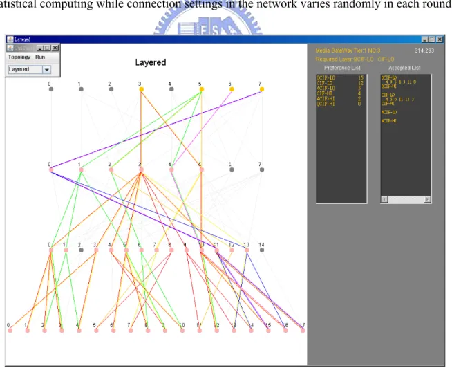
(38) Chapter 6. 6.1. Experiments. Platform. The simulation [Figure 6] is programmed in JAVA with different algorithm implemented in different node classes but in the same randomized network architecture in each execution of the program. The operation system that the simulation executed on is Fedora 8. The simulation will be executed in 100 times in each network congestion case to do some statistical computing while connection settings in the network varies randomly in each round.. Figure 6: Graphic User Interface of Simulation for Bandwidth Reservation Protocol 29.

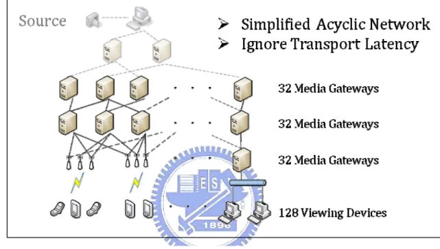
(39) 6.2. Models. 6.2.1 Network Model. Figure 7: Network Model In our simulation experiments, we devised a simple multicast mesh with three tiers as in [Figure 7], named as Tier 0, Tier 1, and Tier 2. User devices are placed at the leaf nodes of the mesh and the media gateways (MGs) serve as the intermediate nodes. There are a total of 128 user devices placed in eight Tier-0 local subnets. Hence, the MGs in Tier 1 broadcast their data flows while the MRs in Tier 2 relay data using unicast communication. Each MG has a restricted outbound bandwidth that it can use to serve its subscribers. We implemented a randomized request mechanism in our simulation. When subscribers are making requests, they see those providers with no difference. So they just choose to send requests randomly with random layers that they require. We run experiments both on the 30.

(40) mesh and tree network model. Devices are subscribing to the clip and running the resource allocation on the network. We tune the Demand/Capacity Ratio as the network congestion factor. Demand is the total bitrates of the devices if they require AVC clips and Capacity are the total outbound bandwidth of the media relays in the local network. We run our experiments to figure out how our mechanisms run under such the network condition of AVC Simulcast.. 31.

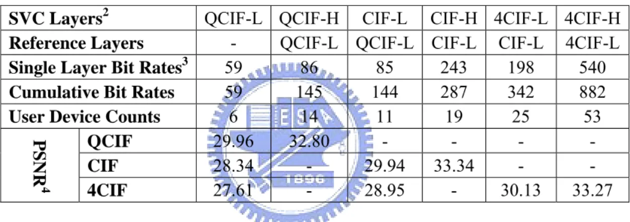
(41) 6.2.2 Source Model. The movie clip we use is “crew” and its length is 10 seconds. We have a base layer and 5 enhancement layers, named QCIF-Low (Base Layer), QCIF-High, CIF-Low, CIF-High, 4CIF-Low, 4CIF-High (Enhancement Layers), and the dependency tree are as below. We choose the QP=6 and calculate the bit-rate of each layer by JSVM. The user devices may be 6 types as above, so they just subscribe layers based on its capability. Detail information is shown in [Table 6] and the dependency relationship is shown in [Figure 8].. PSNR4. QCIF-L QCIF-H CIF-L CIF-H 4CIF-L 4CIF-H SVC Layers2 QCIF-L QCIF-L CIF-L CIF-L 4CIF-L Reference Layers 3 59 86 85 243 198 540 Single Layer Bit Rates 59 145 144 287 342 882 Cumulative Bit Rates 6 14 11 19 25 53 User Device Counts 29.96 32.80 QCIF 28.34 29.94 33.34 CIF 27.61 28.95 30.13 33.27 4CIF Table 6: Characteristics of SVC test bitstream. Figure 8: Dependency Relationship. 2 3 4. The SVC bitstream used in our simulation experiments was a ten-second clipping of the test video, crew. The unit of bit rate measurements is Kilo-bytes per second. The SVC bitstream was encoded using JSVM v.9 with a Qp value of six (6) between each adjacent layer. 32.

(42) Chapter 7. Results and Analysis. Conforming to the comparative study conducted by T.H. Kim [3], we show the performance of our SVC multicasting scheme by displaying the values of four main parameters: PSNR reduction, transport efficiency, bandwidth consumption by individual SVC layer, and average media relay bandwidth utilization. We run the experiment 100 times in fifteen network congestion cases from 60% to 200% which is the X-axis in all our diagrams. The error bars show the ranges of data between 10th and 90th percentiles in one hundred simulation rounds. In these figures, the red dash lines mark where the transport capacity of each MG equals to the total bit rate (1211 kbps) of the SVC bitstream. The blue dash lines mark where the MR capacity equals to the bit rate of the largest decodable bitstream (882 kbps of 4CIF-H layer). We set the amounts 6, 14, 11, 19, 25, 53 for six different devices. The population distribution is quite different from the layer characteristic. There are many 4CIF devices but they are the heaviest load in the network, which means the largest bit rates but the least PSNR improvement. We will show the results of our four different algorithms, a randomized algorithm, and two different AVC algorithms. The first one is the competing AVC algorithm. The behavior of our algorithm 1, 2, and 3 are all the same with AVC. All different layers of AVC compete in the network at the same time. And another one is the dominated AVC which is just like our algorithm 4. MGs pick a dominated AVC layer in the local subnet at once. 33.

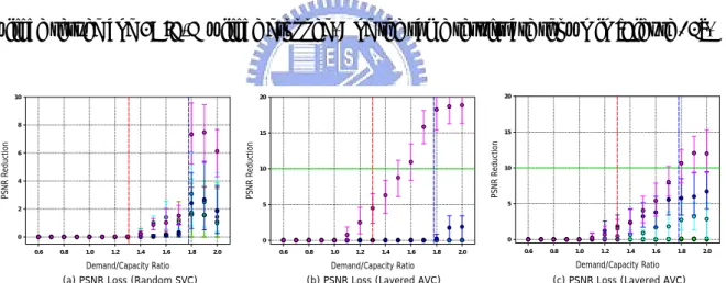
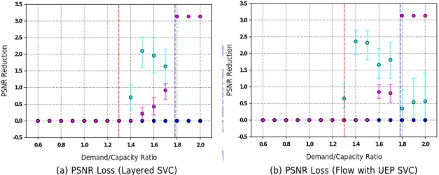
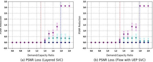
(43) The colors for QCIF-L, QCIF-H, CIF-L, CIF-H, 4CIF-L and 4CIF-H are red, yellow, green, cyan, blue, and magenta in order.. 7.1. PSNR Reduction. PSNR Reduction of viewing devices is the most intuitive factor that users may concern. This measurement will show us the average distortion for each kind of devices. Compare [Figure 9] to other figures of our algorithms, we will find that what we have proposed perform much better than the natural randomized algorithm, the competing AVC, and the dominated AVC algorithm. For devices running randomized algorithm, all layers have probability to be dropped and the probability is proportion to the population distribution. For devices running AVC algorithms, there are only two results of any device, that is, received and not received. So the PSNR Reduction results shown in AVC algorithms vary from a large range. In competing AVC algorithm, all layers compete at the same time, so the 4CIF-L which has higher bit-rates but not as much PSNR improvement will be the worst one. But in dominated AVC algorithm, only one layer at once in local subnets cause 4CIF-H layer which has the largest population performs not so bad as competing AVC one. It shows that in some subnets other layers will be dropped to serve more 4CIF-H layers. Under this measurement, flows with UEP approach performs a little bit worse than Layered SVC. It is because we have not prune the extra flows introduced by UEP even if devices subscribe successfully. In [Figure 10] [Figure 12], the PSNR reduction is almost the same in either Layered SVC or Flows with UEP cases. It is because the characteristics of layers what we encoded cause that. 34.

(44) the order of algorithm 1 is same as algorithm 3. In algorithm 1, the order is {QCIF-L, CIF-L, QCIF-H, CIF-H, 4CIF-L, 4CIF-H}. And in algorithm 3, the only difference is that CIF-L and QCIF-L will compete at the same time and CIF-H and 4CIF-L will compete at the same time. Since the bandwidth is quite enough as they are competing, it makes almost no difference in these two algorithms. We start to drop 4CIF-H layers after the red dash line. It means that there are no any MG could serve all six layers at the same time. After blue dash line, we can no longer serve a complete 4CIF-H device. So they can at most receive a 4CIF-L bitstreams. In [Figure 11], we compare algorithm 2 with algorithm 1. Since algorithm 2 will take population into consideration, so 4CIF-H devices’ quality drops less but some CIF-H devices’ quality drops. But after the blue dash line, all 4CIF-H layers could no longer be served, CIF-H will be served and 4CIF-H will be dropped. And the same results are shown in [Figure 13].. 10. 20. 20. 15. 15. 6. 4. PSNR Reduction. PSNR Reduction. PSNR Reduction. 8. 10. 5. 5. 2. 0. 0. 0 0.6. 0.8. 1.0. 1.2. 1.4. 1.6. 1.8. 2.0. 10. 0.6. 0.8. 1.0. 1.2. 1.4. 1.6. 1.8. 2.0. 0.6. 0.8. 1.0. 1.2. 1.4. 1.6. 1.8. Demand/Capacity Ratio. Demand/Capacity Ratio. Demand/Capacity Ratio. (a) PSNR Loss (Random SVC). (b) PSNR Loss (Layered AVC). (c) PSNR Loss (Layered AVC). Figure 9: PSNR Reduction. 35. 2.0.

(45) 3.5. 3.0. 3.0. 2.5. 2.5. PSNR Reduction. PSNR Reduction. 3.5. 2.0 1.5 1.0. 2.0 1.5 1.0. 0.5. 0.5. 0.0. 0.0. -0.5. -0.5 0.6. 0.8. 1.0. 1.2. 1.4. 1.6. 1.8. 2.0. 0.6. 0.8. 1.0. 1.2. 1.4. 1.6. 1.8. Demand/Capacity Ratio. Demand/Capacity Ratio. (a) PSNR Loss (Layered SVC). (b) PSNR Loss (Flow with UEP SVC). 2.0. 3.5. 3.5. 3.0. 3.0. 2.5. 2.5. PSNR Reduction. PSNR Reduction. Figure 10: PSNR Reduction of Algorithm 1. 2.0 1.5 1.0. 2.0 1.5 1.0. 0.5. 0.5. 0.0. 0.0 -0.5. -0.5 0.6. 0.8. 1.0. 1.2. 1.4. 1.6. 1.8. 0.6. 2.0. 0.8. 1.0. 1.2. 1.4. 1.6. 1.8. 2.0. Demand/Capacity Ratio. Demand/Capacity Ratio. (a) PSNR Loss (Layered SVC). (b) PSNR Loss (Flow with UEP SVC). 3.5. 3.5. 3.0. 3.0. 2.5. 2.5. PSNR Reduction. PSNR Reduction. Figure 11: PSNR Reduction of Algorithm 2. 2.0 1.5 1.0. 2.0 1.5 1.0. 0.5. 0.5. 0.0. 0.0. -0.5. -0.5 0.6. 0.8. 1.0. 1.2. 1.4. 1.6. 1.8. 2.0. 0.6. Demand/Capacity Ratio. 0.8. 1.0. 1.2. 1.4. 1.6. 1.8. Demand/Capacity Ratio. (b) PSNR Loss (Flow with UEP SVC). (a) PSNR Loss (Layered SVC). Figure 12: PSNR Reduction of Algorithm 3 36. 2.0.

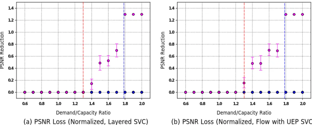
(46) 3.5. 3.0. 3.0. 2.5. 2.5. PSNR Reduction. PSNR Reduction. 3.5. 2.0 1.5 1.0. 2.0 1.5 1.0. 0.5. 0.5. 0.0. 0.0. -0.5. -0.5 0.6. 0.8. 1.0. 1.2. 1.4. 1.6. 1.8. 2.0. 0.6. 0.8. 1.0. Demand/Capacity Ratio. 1.2. 1.4. 1.6. 1.8. 2.0. Demand/Capacity Ratio. (a) PSNR Loss (Layered SVC). (b) PSNR Loss (Flow with UEP SVC). Figure 13: PSNR Reduction of Algorithm 4. 7.2. Normalized PSNR Reduction. The first measurement shows the playback quality of devices, but it can not show the influence about the population of viewing devices. PSNR loss means quite different in a large population from a small one. We multiply PSNR reduction by percentage of specific device’s population in whole population. In [Figure 14] [Figure 15] [Figure 17] [Figure 18], the results almost show the same as the first measurement but we can see clearly in [Figure 16], normalized PSNR reduction in 4CIF-H is lower than other algorithms but almost the same as. 5. 5. 4. 4. 4. 3. 2. PSNR Reduction. 5. PSNR Reduction. PSNR Reduction. CIF-H. It shows how we compromise between layers.. 3. 2. 1. 1. 0.6. 0.8. 1.0. 1.2. 1.4. 1.6. 1.8. 2.0. 2. 1. 0. 0. 3. 0. 0.6. 0.8. 1.0. 1.2. 1.4. 1.6. 1.8. 2.0. 0.6. Demand/Capacity Ratio. Demand/Capacity Ratio. (a) PSNR Loss (Normalized, Random SVC). (b) PSNR Loss (Normalized, Layered AVC). 1.0. 1.2. 1.4. 1.6. 1.8. 2.0. Demand/Capacity Ratio. (c) PSNR Loss (Normalized, Layered AVC). Figure 14: Normalized PSNR Reduction 37. 0.8.

(47) 1.4. 1.2. 1.2. 1.0. 1.0. PSNR Reduction. PSNR Reduction. 1.4. 0.8 0.6 0.4. 0.8 0.6 0.4. 0.2. 0.2. 0.0. 0.0 0.6. 0.8. 1.0. 1.2. 1.4. 1.6. 1.8. 2.0. 0.6. 0.8. Demand/Capacity Ratio. 1.0. 1.2. 1.4. 1.6. 1.8. 2.0. Demand/Capacity Ratio. (a) PSNR Loss (Normalized, Layered SVC). (b) PSNR Loss (Normalized, Flow with UEP SVC). 1.4. 1.4. 1.2. 1.2. 1.0. 1.0. PSNR Reduction. PSNR Reduction. Figure 15: Normalized PSNR Reduction of Algorithm 1. 0.8 0.6 0.4. 0.8 0.6 0.4. 0.2. 0.2. 0.0. 0.0 0.6. 0.8. 1.0. 1.2. 1.4. 1.6. 1.8. 0.6. 2.0. 0.8. 1.0. 1.2. 1.4. 1.6. 1.8. 2.0. Demand/Capacity Ratio. Demand/Capacity Ratio. (b) PSNR Loss (Normalized, Flow with UEP SVC). (a) PSNR Loss (Normalized, Layered SVC). 1.4. 1.4. 1.2. 1.2. 1.0. 1.0. PSNR Reduction. PSNR Reduction. Figure 16: Normalized PSNR Reduction of Algorithm 2. 0.8 0.6 0.4. 0.8 0.6 0.4. 0.2. 0.2. 0.0. 0.0 0.6. 0.8. 1.0. 1.2. 1.4. 1.6. 1.8. 2.0. 0.6. Demand/Capacity Ratio. 0.8. 1.0. 1.2. 1.4. 1.6. 1.8. 2.0. Demand/Capacity Ratio. (a) PSNR Loss (Normalized, Layered SVC). (b) PSNR Loss (Normalized, Flow with UEP SVC). Figure 17: Normalized PSNR Reduction of Algorithm 3 38.

(48) 1.5. 1.0. 1.0. PSNR Reduction. PSNR Reduction. 1.5. 0.5. 0.5. 0.0. 0.0 0.6. 0.8. 1.0. 1.2. 1.4. 1.6. 1.8. 0.6. 2.0. 0.8. 1.0. 1.2. 1.4. 1.6. 1.8. 2.0. Demand/Capacity Ratio. Demand/Capacity Ratio. (a) PSNR Loss (Normalized, Layered SVC). (b) PSNR Loss (Normalized, Flow with UEP SVC). Figure 18: Normalized PSNR Reduction of Algorithm 4. 7.3. SVC vs. AVC. This measurement is going to show us the benefit we gain from using SVC rather than AVC. We can see clearly in [Figure 19].. 39.

(49) 20. 15. 15. PSNR Reduction. PSNR Reduction. 20. 10. 5. 0. 10. 5. 0. -5. -5 0.6. 0.8. 1.0. 1.2. 1.4. 1.6. 1.8. 2.0. 0.6. 0.8. Demand/Capacity Ratio. 1.2. 1.4. 1.6. 1.8. 2.0. Demand/Capacity Ratio. (a) PSNR Loss (Difference, Layered). (b) PSNR Loss (Difference, Layered). 20. 20. 15. 15. PSNR Reduction. PSNR Reduction. 1.0. 10. 5. 0. 10. 5. 0. -5. -5. 0.6. 0.8. 1.0. 1.2. 1.4. 1.6. 1.8. 2.0. 0.6. Demand/Capacity Ratio. 0.8. 1.0. 1.2. 1.4. 1.6. 1.8. 2.0. Demand/Capacity Ratio. (c) PSNR Loss (Difference, Layered). (d) PSNR Loss (Difference, Layered). Figure 19: Difference between SVC and AVC of four algorithms. 7.4. Efficiency. Efficiency is going to show how the mechanism works. It is calculated by the total bitrates that devices receive divided by the total bitrates of traffic flow in every links on the network. Because of the broadcast at the bottom tier, the efficiency may be larger than 1. We measure the efficiency instead of the sum of bitrates on the network because if the user devices get less, the sum of bitrates on the network will be less relatively. To avoid misleading this, we measure the efficiency. Since the same reason, flows with UEP approach performs not as well as Layered SVC approach due to the extra flows. 40.

(50) The Efficiency is almost always at 1 even larger than 1 after the blue dash line. It is because 4CIF-H is the most inefficient. Layered SVC approach performs much better than other approaches in [Figure 20].. 1.2. 1.2. 1.0. Efficiency. Efficiency. 1.0. 0.8. 0.6. 0.6. 0.4. 0.4 0.6. 0.8. 1.0. 1.2. 1.4. 1.6. 1.8. 0.6. 2.0. 0.8. 1.0. 1.2. 1.4. Demand/Capacity. Demand/Capacity. (a) Efficiency. (b) Efficiency. 1.2. 1.2. 1.0. 1.0. Efficiency. Efficiency. 0.8. 0.8. 1.6. 1.8. 2.0. 1.6. 1.8. 2.0. 0.8. 0.6. 0.6. 0.4. 0.4 0.6. 0.8. 1.0. 1.2. 1.4. 1.6. 1.8. 0.6. 2.0. 0.8. 1.0. 1.2. 1.4. Demand/Capacity. Demand/Capacity. (c) Efficiency. (d) Efficiency. Figure 20: Efficiency for four algorithms. 7.5. Layer Bandwidth Ratio. Layer Bandwidth Ratio is about the amount of each layer in each tier. This may show the aggregation of layers between tiers. The original demand amount of layers and amount of layers broadcasted is shown in [Table 7]. And in [Figure 21] [Figure 22] [Figure 23] [Figure. 41.

(51) 24], we show the amount of layers between the medium tier and the top tier. Layers in the network are reduced from 1/2 to 1/6.. QCIF-L QCIF-H CIF-L CIF-H 4CIF-L 4CIF-H Original Device Demand. 128. 14. Between Bottom & Medium Tier 31.42. 108. 19. 78. 53. 10.22 31.26 13.34 29.34. 24.93. 40. 40. 35. 35. Layer Bandwidth Ratio. Layer Bandwidth Ratio. Table 7: Original Layer Counts and Layers Counts in lower tiers. 30 25 20 15 10 5. 30 25 20 15 10 5. 0. 0. 0.6. 0.8. 1.0. 1.2. 1.4. 1.6. 1.8. 2.0. 0.6. 0.8. Demand/Capacity Ratio. 1.0. 1.2. 1.4. 1.6. 1.8. 2.0. Demand/Capacity Ratio. (a) Layer Bandwidth Ratio (Layered SVC). (b) Layer Bandwidth Ratio (Flow with UEP SVC). 40. 40. 35. 35. Layer Bandwidth Ratio. Layer Bandwidth Ratio. Figure 21: Layer Bandwidth Ratio of Algorithm 1. 30 25 20 15 10 5. 30 25 20 15 10 5. 0. 0 0.6. 0.8. 1.0. 1.2. 1.4. 1.6. 1.8. 2.0. 0.6. Demand/Capacity Ratio. 0.8. 1.0. 1.2. 1.4. 1.6. Demand/Capacity Ratio. (a) Layer Bandwidth Ratio (Layered SVC). 1.8. 2.0. (b) Layer Bandwidth Ratio (Flow with UEP SVC). Figure 22: Layer Bandwidth Ratio of Algorithm 2 42.

(52) 40. 35. 35. Layer Bandwidth Ratio. Layer Bandwidth Ratio. 40. 30 25 20 15 10 5. 30 25 20 15 10 5. 0. 0 0.6. 0.8. 1.0. 1.2. 1.4. 1.6. 1.8. 2.0. 0.6. 0.8. Demand/Capacity Ratio. 1.0. 1.2. 1.4. 1.6. 1.8. 2.0. Demand/Capacity Ratio. (a) Layer Bandwidth Ratio (Layered SVC). (b) Layer Bandwidth Ratio (Flow with UEP SVC). 40. 40. 35. 35. Layer Bandwidth Ratio. Layer Bandwidth Ratio. Figure 23: Layer Bandwidth Ratio of Algorithm 3. 30 25 20 15 10 5. 30 25 20 15 10 5. 0. 0. 0.6. 0.8. 1.0. 1.2. 1.4. 1.6. 1.8. 2.0. 0.6. Demand/Capacity Ratio. 0.8. 1.0. 1.2. 1.4. 1.6. 1.8. 2.0. Demand/Capacity Ratio. (a) Layer Bandwidth Ratio (Layered SVC). (b) Layer Bandwidth Ratio (Flow with UEP SVC). Figure 24: Layer Bandwidth Ratio of Algorithm 4. 7.6. Average Media Gateway Bandwidth Usage. Average Media Gateway Bandwidth Usage shows the load of MGs in each tier and we can figure out whether MGs are used well or not. Since some MGs may be unused because of the aggregation of layers, this measurement will tell us how we use the bandwidth in those used MGs (active MGs). Colors that represent top, medium, and bottom tiers are blue, green, and red. In [Figure 25] [Figure 26] [Figure 27] [Figure 28] [Figure 29], we can find that we use 43.

(53) MGs better than randomized algorithm and AVC algorithms. Use most bandwidth of MGs in the medium tier where aggregation happens most and the tier with heaviest load in the network. But we use less in the top tier due to the aggregation. Figures of flows with UEP approach show us how flows can almost be filled in all active MGs’ capacity.. 0.6. 0.4. 0.2. 0.0. 1.0. Average MR Bandwidth Usage. Average MR Bandwidth Usage. 1.0. 0.8. 0.8. 0.6. 0.4. 0.2. 0.0 0.6. 0.8. 1.0. 1.2. 1.4. 1.6. 1.8. 2.0. 0.8. 0.6. 0.4. 0.2. 0.0 0.6. 0.8. 1.0. 1.2. 1.4. 1.6. 1.8. 2.0. 0.6. 0.8. 1.0. 1.2. 1.4. 1.6. 1.8. Demand/Capacity Ratio. Demand/Capacity Ratio. Demand/Capacity Ratio. (a) MG Avg Load (Random SVC). (b) MG Avg Load (Layered AVC). (c) MG Avg Load (Layered AVC). Figure 25: Average Media Gateway Bandwidth Usage of algorithms 1.0. Average MR Bandwidth Usage. 1.0. Average MR Bandwidth Usage. Average MR Bandwidth Usage. 1.0. 0.8. 0.6. 0.4. 0.2. 0.0. 0.8. 0.6. 0.4. 0.2. 0.0 0.6. 0.8. 1.0. 1.2. 1.4. 1.6. 1.8. 2.0. 0.6. 0.8. 1.0. 1.2. 1.4. 1.6. 1.8. 2.0. Demand/Capacity Ratio. Demand/Capacity Ratio. (a) MG Avg Load (Layered SVC). (b) MG Avg Load (Flow with UEP SVC). Figure 26: Average Media Gateway Bandwidth Usage of Algorithm 1. 44. 2.0.

(54) 1.0. Average MR Bandwidth Usage. Average MR Bandwidth Usage. 1.0. 0.8. 0.6. 0.4. 0.2. 0.0. 0.8. 0.6. 0.4. 0.2. 0.0 0.6. 0.8. 1.0. 1.2. 1.4. 1.6. 1.8. 2.0. 0.6. 0.8. 1.0. 1.2. 1.4. 1.6. 1.8. 2.0. Demand/Capacity Ratio. Demand/Capacity Ratio. (a) MG Avg Load (Layered SVC). (b) MG Avg Load (Flow with UEP SVC). Figure 27: Average Media Gateway Bandwidth Usage of Algorithm 2 1.0. Average MR Bandwidth Usage. Average MR Bandwidth Usage. 1.0. 0.8. 0.6. 0.4. 0.2. 0.0. 0.8. 0.6. 0.4. 0.2. 0.0 0.6. 0.8. 1.0. 1.2. 1.4. 1.6. 1.8. 2.0. 0.6. 0.8. 1.0. 1.2. 1.4. 1.6. 1.8. 2.0. Demand/Capacity Ratio. Demand/Capacity Ratio. (a) MG Avg Load (Layered SVC). (b) MG Avg Load (Flow with UEP SVC). Figure 28: Average Media Gateway Bandwidth Usage of Algorithm 3 1.0. Average MR Bandwidth Usage. Average MR Bandwidth Usage. 1.0. 0.8. 0.6. 0.4. 0.2. 0.0. 0.8. 0.6. 0.4. 0.2. 0.0 0.6. 0.8. 1.0. 1.2. 1.4. 1.6. 1.8. 2.0. 0.6. 0.8. 1.0. 1.2. 1.4. 1.6. 1.8. 2.0. Demand/Capacity Ratio. Demand/Capacity Ratio. (a) MG Avg Load (Layered SVC). (b) MG Avg Load (Flow with UEP SVC). Figure 29: Average Media Gateway Bandwidth Usage of Algorithm 4. 45.

(55) Chapter 8. 8.1. Conclusion. Accomplishment. We proposed a new scheme for streaming video based upon SVC Multicasting. We can serve not only with better playback quality but also in an efficient way to transport. And we show that SVC performs better than AVC if we can transfer layers in a correct way. We proposed an optimization model, z. Rate-Distortion Gain: To optimize R-D gain will make the multicasting have better playback quality and decrease the network bandwidth consumption.. We proposed a four way handshake bandwidth allocation protocol and implemented a complete simulation for our scheme and had results as following, z. Well performed in Playback Quality.. z. Higher Efficiency for network bandwidth consumption.. z. Do Aggregation in media gateways.. z. Use media gateways’ bandwidth well.. z. SVC Multicasting performs much better than AVC Simucasting.. 46.

(56) 8.2. Future Work. We shall attempt to estimate the average performance of Rate-Distortion Gain our distributed bandwidth allocation algorithm using stochastic models and devise modification to the proposed algorithms in order to avoid local optima. We will consider not only bandwidth but also latency and error in the future and implement it on a network simulator such as OMNeT++.. 47.

(57) Glossary Symbols. Definitions. L. Layer ID as concatenation of Dependency ID, Quality ID and Temporal ID of SVC NAL Units. U( ). Type of User Device with target SVC layers set. nU. Number of Devices U( ) in the network. nU. ,. .. Number of Devices U( ) in the sub-tree whose root is MG ,. T. Total Tier Numbers.. MG ,. jth Media Gateway in Tier i. D. jth User Device (as a leaf of SVC multicast tree). ξ ,. Fan In of MG ,. RepCount , , L. Replication Count of Layer L at MG ,. LayerCount A ,. , ,L. Allowed Layer Count of Layer L at MG , Children Set of MGs that is accessible to MG ,. L. Layer ID of Serving Layer L. Device Type Set of all device types that need L. D. Set of all layers that D. needs. d U. ,L. PSNR Improvement of Device Type U. d D. ,L. PSNR Improvement of Device D. receiving Layer L. r L. Bit rate of Layer L. γ , ,L. Rate-Distortion Gain of MG ,. γ L. Rate-Distortion Gain of allocating Layer L. γ D. ,L. Rate-Distortion Gain of D. γ E. receiving Layer L. receiving Layer L. receiving Layer L. Total Rate-Distortion Gain 1, ; , ; L. Expectation Value of number of layer L that subscriber MG ,. could get from provider MG. 48. 1,. ..

(58) References [1] T. Wiegand, G. Sllivan, J. Reichel, H. Schwarz, M.Wien. “Joint Draft ITUT Rec.H.264 – ISO/IEC 14496-10/ Amd.3 Scalable Video Coding,” ISO/IEC/JTCI/SC29/ WG-11 and ITU-T SG16 Q.6, JVT-X201, July 2007. [2] H. Schwarz, D. Marpe, and T. Wiegand, “Overview of the Scalable Video Coding Extension of the H.264/AVC Standard,” IEEE TRANSACTIONS on CIRCUITS AND SYSTEMS FOR VIDEO TECHNOLOGY, VOL. 17, NO. 9, September 2007. [3] T. H. Kim, “Scalable Video Streaming over Internet”. PhD Thesis, School of Electrical and Computer En-gineering, Georgia Institute of Technology, January 2005 [4] S. Y. Cheung, M. H. Ammar, and X. Li, “On the use of destination set grouping to improve fairness in multicast video distribution,” IEEE INFOCOM ’96, San Francisco, CA, Mar. 1996. [5] T. Jiang, M. H. Ammar, and E. W. Zegura, “Inter-receiver fairness: a novel performance measure for multicast ABR sessions,” ACM SIGMETRICS ＇98, Madison, WI, June 1998. [6] X. Li, S. Paul, and M. H. Ammar, “Layered video multicast with retransmission (LVMR): Evaluation of hierarchical rate control,” IEEE INFOCOM ’98, San Francisco, CA, Mar. 1998. [7] S. McCanne, V. Jacobson, and M. Vetterli, “Receiver driven layered multicast,” ACM SIGCOMM ’96, Stanford, CA, Aug. 1996. [8] J. Byers, M. Luby, and M. Mitzenmacher, “Fine-grained layered multicast,” IEEE INFOCOM 2001, Anchorge, AK, Apr. 2001. [9] V. K. Goyal, J. Ko˘cevi′c, R. Arean, and M. Vetterli, “Multiple description transform coding of images,” ICIP ’98, Chicago, IL, Oct. 1998. [10] P. Baccichet, T. Schierl, T. Wiegand, B. Girod. “Low Delay Peer-to-Peer Streaming using Scalable Video Coding”. Proc. IEEE International Conference on Image Processing (ICIP) 2007, pp. 1-22, 2007. 49.

(59) [11] S. Wee, J. Apostolopoulos, W. Tan, S. Roy. “Research and Design of a Mobile Streaming Media Content Delivery Network”. Proc. IEEE ICME 2003. [12] M. Castro, P. Druschel, A.-M. Kermarrec, A. Nandi, A. Rowstron, A. Singh, “SplitStream: High-bandwidth content distribution in a cooperative environment,” Proc. IPTPS’03, Berkeley, CA, Feburary 2003. [13] Y. H. Guo, J. K. Zao, W. H. Peng, L. S. Huang, C. M. Lin, F. P. Kuo. “Trickle: Resilient Real-Time Video Multicasting for Dynamic Peers with Limited or Asymmetric Network Connectivity”. Proc. IEEE Int’l Symposium on Multimedia (ISM), San Diego, CA, December 2006. [14] A. Segall. “SVC-to-AVC Bit-Stream Rewriting for Coarse Grain Scalability”. Joint Video Team, doc. JVT-V035, Marrakech, Morocco, January 2007.. 50.

(60)