貝氏階層式結構於視訊監控之研究與應用

國立交通大學

電子工程學系電子研究所

博 士 論 文

貝氏階層式結構於視訊監控之研究與應用

A Study of Bayesian Hierarchical Framework

and Its Applications to Video Surveillance

研

究

生：黃敬群

指 導 教 授：王聖智 博士

貝氏階層式結構於視訊監控之研究與應用

A Study of Bayesian Hierarchical Framework and Its Applications

to Video Surveillance

研 究 生：黃敬群

Student: Ching-Chun Huang

指導教授：王聖智 博士 Advisor:

Dr.

Sheng-Jyh

Wang

國 立 交 通 大 學

電 子 工 程 學 系 電 子 研 究 所 博 士 班

博 士 論 文

A Dissertation Submitted to

Department of Electronics Engineering & Institute of Electronics

College of Electrical Engineering and Computer Engineering

National Chiao Tung University

in Partial Fulfillment of the Requirements

for the Degree of

Doctor of Philosophy

in

Electronics Engineering

September 2010

Hsinchu, Taiwan, Republic of China

貝氏階層式結構於視訊監控之研究與應用

研究生：黃敬群 指導教授：王聖智博士

國立交通大學電子工程學系電子研究所 博士班

摘要

在本論文中，我們提出以貝氏階層式結構為基礎的分析方法，讓視訊監控系 統得以用一致的架構，同時分析影像內容以及推論空間中場景的資訊。在真實的 場景中，為了實現一套穩健的視訊監控系統，往往會面臨許多挑戰，諸如物體間 相互遮蔽、前景物體與背景物體外貌相似而產生的混淆、透視投影所造成的物體 形變、陰影的變化、還有外在光線變化造成的影像變異。在這篇論文中，我們發 現，透過將空間場景適當的參數化，並同時依據場景模型和擷取到的影像資料來 進行分析，系統將能更輕易地處理前面所提及的變異因素。在貝氏階層式架構 中，我們透過階層式表示法將以像素特徵為基礎的資訊、以區域影像內容為基礎 的資訊、與以物件特性為基礎的資訊，透過機率的方式進行有系統的整合，以支 援影像內容的分析與場景資訊的推論。透過所提出的貝氏階層式架構，前面所提 到的許多變異因素可以被有效地解決，除此之外，某些變異因素還可進一步變成 有效的線索來協助三維場景資訊的推論。 在本論文中，我們將貝氏階層式架構實際應用在停車場空位偵測系統以及多 攝影機視訊監控系統。在停車場空位自動偵測的系統上，實際的戶外停車場監控 場景往往受到許多變因的影響，進而降低了系統的正確性，這些變因包含: (a)戶 外變化劇烈的環境光源; (b)陰影的影響; (c)透視法上幾何投影所產生的變形; (d) 停放車輛之間產生的相互遮蔽問題。藉由所提出的貝氏階層式結構，我們可以有

系統地將前述的許多變因加入停車空位的推論過程中，以降低這些變因對系統效 能的影響。我們的貝氏階層式結構透過建立參數化的空間場景模型來描述空間中 的遮蔽現象、幾何上的投影變形、以及陰影等變因所形成的影響，同時也將環境 光線變化所造成的色彩變動視為一種色彩分類的問題，並藉由分類程序的建立來 描述光線的變化。實驗結果顯示，我們的系統可以穩定地偵測空位的位置、有效 地標記並區分影像中屬於地面或車輛的區域、確切地標記屬於陰影的區域、以及 克服光線變化所衍生的問題。 另一方面，在多攝影機視訊監控系統中，我們自動地定位、標記、與對應在 不同攝影機監控範圍內的多個物體，同時有效壓抑因為幾何深度上的不確定性所 產生的假物體。多攝影機視訊監控系統在真實的應用場景中，往往面臨一些具挑 戰性的議題: (a) 場景中未知物體的數量; (b)物體間的相互遮蔽; 以及(c)假物體 的出現。有別於過去的方法，我們提出了一套包含資訊整合與場景推論的兩步驟 策略。在資訊整合的步驟中，我們整合來自多攝影機的資訊以建立一機率分佈， 藉以描述物體出現於地面某一位置的可能性。在場景推論的步驟中，我們應用貝 氏階層式結構將場景模型納入考量，透過此結構，我們將物件在影像內的標記議 題、物件在多攝影機間的對應議題、以及假物件的消除議題整合為單一的最佳化 問題。此外，我們進一步採用期望-最大化架構來調整出更好的物體三維模型， 透過貝氏階層式結構與期望-最大化架構的結合，我們可以得到更好的系統效 能。實驗結果顯示，我們的系統可以自動地決定場景中的運動物體數量、有效地 標記並對應出不同攝影機影像中的多個物體、準確地定位物體在三維場景中的位 置、並且能有效地清除假物件。 在本論文中，我們驗證了以貝氏階層式結構為基礎的影像分析架構可以有效 地應用到視訊監控的分析與應用上。透過此架構，我們將像素層級的色彩資訊、 像素間的區域層級資訊、以及以物體為基本單位的物件層級資訊有系統地整合在 一起，這樣的整合讓系統可以擁有更多的資訊，並可以針對較複雜的影像內容進 行準確的推論分析。

A Study of Bayesian Hierarchical Framework and Its

Applications to Video Surveillance

Student：Ching-Chun Huang Advisor：Dr. Sheng-Jyh Wang

Department of Electronics Engineering & Institute of Electronics

National Chiao Tung University

Abstract

In this dissertation, we present a Bayesian hierarchical framework (BHF) to simultaneously deal with 3-D scene modeling and image analysis in a unified manner. In practice, to develop a robust video surveillance system, many challenging issues need to be taken into account, such as occlusion effect, appearance ambiguity between foreground and background, perspective effect, shadow effect, and lighting variations. In this dissertation, we find a way to handle these challenging issues by modeling 3-D scene in a parametric form and by integrating scene model and image observation together in the inference process. In the proposed hierarchical framework, we systematically integrate pixel-level information, region-level information, and object-level information in a probabilistic way for the semantic inference of image content and 3-D scene status. Under this BHF framework, occlusion effect, appearance ambiguity, perspective effect, shadow effect, and lighting variations can be well handled. Actually, in the BHF framework, occlusion effect, perspective effect, and shadow effect may even provide useful clues to support 3-D scene inference.

system. In the vacant parking space detection system, the challenges come from dramatic luminance variations, shadow effect, perspective distortion, and the inter-occlusion among vehicles. With the proposed BHF, those issues can be well modeled in a systematic way and can be effectively handled. In detail, the proposed BHF scheme depicts the occlusion pattern, perspective distortion, and shadow effect by building a parametric scene model. On the other hand, the color fluctuation problem caused by luminance variation is treated as a color classification problem. With the BHF scheme, the detection of vacant parking spaces and the labeling of scene status are regarded as a unified Bayesian optimization problem subject to a shadow generation model, an occlusion generation model, and an object classification model. The system accuracy was evaluated by testing over a few outdoor parking lot videos captured from morning to evening. Experimental results showed that the proposed framework can systematically detect vacant parking spaces, efficiently label ground and car regions, precisely locate shadowed regions, and effectively handle luminance variations.

On the other hand, in the application of multi-target detection and tracking over a multi-camera system, the main goal is to locate, label, and correspond multiple targets with the capability of ghost suppression over a multi-camera surveillance system. In practice, the challenges of this kind of system come from the unknown target number, the inter-occlusion among targets, and the ghost effect caused by geometric ambiguity. Instead of directly corresponding objects among different camera views, the proposed framework adopts a fusion-inference strategy. In the fusion stage, we formulate a posterior distribution to indicate the likelihood of having some moving targets at certain ground locations. In the inference stage, the scene model is inputted into the proposed BHF, where the target labeling, target correspondence, and ghost removal are regarded as a unified optimal problem subject to 3-D scene priors, target priors,

and image observations. Moreover, the target priors are iteratively refined based on an expectation-maximization (EM) process to further improve the system performance. The system accuracy is evaluated via both synthesized videos and real videos. Experimental results showed that the proposed system can systematically determine the target number, efficiently label and correspond moving targets, precisely locate their 3-D locations, and effectively tackle the ghost problem.

With simulations over these two applications, we verified that the proposed BHF scheme can be well applied to various kinds of video surveillance applications. This BHF framework provides the flexibility to properly integrate pixel-level, region-level, and object-level information into a unified inference process. With the integrated information from multiple aspects, we will be able to handle more complicated tasks with improved accuracy and robustness.

Acknowledgements

從小學、中學、一直到博士的學習過程，我需要感謝每一位無私而慷慨指導 我的導師。在這些敬愛的老師中，影響我最深，教導我最多，支持我最久，就是 我的指導教授王聖智博士。在我的腦海中，老師對我的指導，早在高中推薦甄試 後，收到老師寄來一本“電腦系統＂的原文書便已開始;在大學專題實作與研究 所學習時，老師幾乎是亦步亦趨地扶著學生，教我如何做研究;當我開始研習博 士學程時，老師總是不遲辛苦地牽著學生的手，一字一句地教導如何寫論文。十 多年的學習歲月，我何等幸運可以得到王老師無數的關懷與包容，以及數不盡的 疼愛與教誨。印象中的老師，堅毅、認真、嚴謹、而且仁慈。學者的風範，深刻 地影響著我，在無所適從的時刻，正因著老師的精神與我同伴，得以尋得正確的 方向。真的非常感謝老師的栽培，謝謝老師。 能夠完成學業，我還要感謝我的家人，特別是我的母親---傅玉女女士。感 謝母親的教養與督促，總是在我洩氣時給我重新站起來的力量;在我做決定時給 予我適時的建議與全部的信任;感謝母親在生活與精神上全力的支持。也要感謝 珮婷，在最艱苦的時刻，給我絕對的肯定與滿滿的歡笑。 此外，我要感謝實驗室的許多好伙伴。沒有您們的支持與陪伴，研究生活中 必然缺少調色而黯淡非常。感謝熱心的奕安與瑞男，可愛又聰明的晴駿，貼心又 搞笑的維辰和庭瑋，認真負責的博凱、瑋國、周節、禎宇，以及老是聽我訴苦的 慈澄。還有許許多多學弟妹，您們真是太棒啦! 另外，工研院以及遠在美國卡內基大學的許多師長與朋友，感謝您們讓我的 生命更寬廣。感謝陳祖翰教授、張耀仁博士的指導;感謝余孝先副所長、張森嘉 博士給我工作的機會，發揮所學的舞台，並在我犯錯時包容與教導我。感謝鴻欣、 正一、博超 … 等工作上合作無間的夥伴。 我還要感謝投稿過程中給予我寶貴意見的許多匿名的論文評論委員。我也要 感謝敬愛的博士班口試委員們，洪一平博士、戴顯權博士、黃仲陵博士、張文鍾 博士、莊仁輝博士、許秋婷博士、林嘉文博士以及王聖智博士，很感謝您們的愛 護及教誨。 最後，我要感謝主一路的保守與眷顧，沒有主的陪伴與引領，許多事情都無 法憑自己的力量克服，感謝主，願這得來不易的喜悅，可以彰顯主的光輝與榮耀。 黃敬群 2010 年 9 月

Contents

______________________________________________

摘要 ………... i Abstract... iii Acknowledgements...vi Contents ...vii List of Tables...x

List of Figures ...xi

List of Notations ...xvi

Introduction...1

1.1 Overview...1

1.2 Contribution ...4

1.3 Organization...6

Backgrounds ...7

2.1 Image Analysis Techniques...8

2.1.1 Pixel-level Methods ...8

2.1.2 Region-level Methods...13

2.1.3 Object-level Methods...18

2.2 Connection between Image Analysis and 3D Scene Modeling ...24

Bayesian Hierarchical Framework...28

3.1 The Structure of BHF...28

3.2.2 Differences to Existing Hybrid Methods ...33

3.3 The Modeling of BHF...35

3.4 The Inference of BHF ...41

3.5 The Application of BHF...44

A Hierarchical Bayesian Generation Framework for Vacant Parking Space Detection ……… 46

4.1 Introduction of Parking Space Detection...46

4.2 Overview of Vacant Space Detection...50

4.3 Top-Down Knowledge From Scene Layer ...54

4.3.1 3-D Scene Parameters ...55

4.3.2 Generation of Expected Labeling Maps ...56

4.3.3 Estimation of Sunlight Direction ...60

4.4 Bottom-Up Messages From Observation Layer ...62

4.4.1 Classification Energy Model...63

4.4.2 Adjacency Energy Model ...69

4.5 Vacant Parking Space Detection ...70

4.5.1 Optimal Inference of Parking Space Status ...70

4.5.2 Refinement of Classification Energy Model...72

4.5.3 System Setup and Online Vacant Space Detection ...73

4.6 Experiment Results and Discussion...75

4.6.1 Experiment Setup and Test Data...75

4.6.2 Object/Shadow Labeling and Accuracy of Vacant Space Detection ………..76

4.6.3 Discussion and Future Works ...83

Multi-Target Correspondence and Labeling with Ghost Suppression over Multi-Camera System ...85

5.1 Introduction...85

5.2 System Overview...89

5.2.1 System Property...90

5.2.2 System Flow...91

5.3 Information Fusion and Summarization ...93

5.3.1 Foreground Detection on Single Camera...93

5.3.2 Information Fusion...93

5.3.3 Representation of TDP and Information Summarization...97

5.3.4 Ghost Object ...99

5.4.1 System Modeling ...102

5.4.2 Multi-Target Labeling and Tracking ...107

5.5 Results and Discussion ...114

5.5.1 Experimental Datasets ...114

5.5.2 Foreground Detection and Information Fusion...115

5.5.3 Accuracy of Target Location...119

5.5.4 Detection and Labeling with Ghost Removal...121

5.5.5 Multi-target Tracking on the Ground Plane ...123

5.5.6 System Complexity...124

5.5.7 Future Works...125

Conclusions...126

Bibliography ...133

List of Tables

______________________________________________

TABLE 1. PERFORMANCE COMPARISON OF FOUR VACANT SPACE DETECTION ALGORITHMS. ...82 TABLE 2. ACCURACY OF TARGET LOCATION IN THREE DIFFERENCE ZONES FOR FLEURET’S

SEQUENCE. ...120 TABLE 3. FALSE POSITIVE RATE (FPR), FALSE NEGATIVE RATE (FNR)...122 TABLE 4. RUNTIME LIST...125

List of Figures

______________________________________________

FIG. 1. AN EXAMPLE OF HUMAN DETECTION AND HUMAN IDENTITY LABELING. (A) TEST IMAGE. (B) HUMAN DETECTION RESULT. (C) HUMAN LABELING RESULT, WITH DIFFERENT COLORS INDICATING DIFFERENT PERSONS...2 FIG. 2. THE PROBABILITY DISTRIBUTION OF A PIXEL WITH GAUSSIAN MIXTURE MODEL [2].

...10 FIG. 3. BACKGROUND SUBTRACTION RESULTS BASED ON GAUSSIAN MIXTURE MODEL. 11 FIG. 4. THE BACKGROUND SUBTRACTION RESULTS BASED ON THE METHOD PROPOSED BY

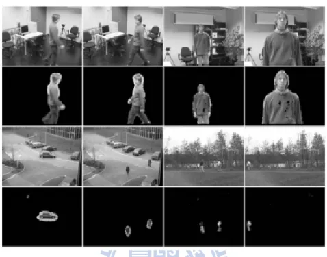
HEIKKILÄ ET AL. [14]. THE FIRST AND THIRD ROWS ARE THE TEST IMAGES. THE SECOND AND FOURTH ROWS ARE THE DETECTION RESULTS. (FIGURES COURTESY OF MARKO HEIKKILÄ [14])...14 FIG. 5. A BACKGROUND SUBTRACTION RESULT BASED ON THE METHOD OF ELGAMMAL

ET AL. [10]. (A) A TEST IMAGE. (B) PER-PIXEL DETECTION RESULT. (C) PER-PIXEL DETECTION RESULT WITH NEIGHBORING CONSIDERATION. (FIGURES COURTESY OF A. ELGAMMAL [10] ) ...15 FIG. 6. THE PROCEDURE FOR THE FOREGROUND MODELING IN [17] BASED ON THE

SPATIAL STATISTICS. (FIGURES COURTESY OF CS. BENEDEK [17]) ...17 FIG. 7. A TYPICAL OBJECT-BASED DETECTION PROCEDURE WITH SLIDING WINDOW. HERE,

WE USE FACE DETECTION AS AN EXAMPLE. ...19 FIG. 8. ILLUSTRATION OF SVM CLASSIFICATION WITH A HYPERPLANE THAT SEPARATES

POSITIVE EXAMPLES (“+”S) FROM NEGATIVE EXAMPLES (“O”S) WITH THE MAXIMUM MARGIN. SUPPORT VECTORS ARE PARTS OF THE TRAINING EXAMPLES THAT LIE ON THE BOUNDARY. ...20 FIG. 9. THE PICTORIAL STRUCTURE FRAMEWORK PROPOSED BY FISCHLER AND

ELSCHLAGER [29]. ...21 FIG. 10. THE PART-BASED OBJECT DETECTION REPORTED IN [32]. (A) A TESTED IMAGE

WITH THE DETECTED HUMAN AND ITS PARTS. (B) THE HOG HUMAN MODEL. (C) THE HOG MODELS OF EACH BODY PARTS. (D) THE DEFORMABLE MODELS

DEPICTING THE POSSIBLE VARIATION OF EACH PART. (FIGURES COURTESY OF P. FELZENSZWALB [32])...22 FIG. 11. FOUR REPRESENTATION METHODS FOR THE HUMAN MODEL. (FIGURES COURTESY

OF JK AGGARWAL [39]) ...23 FIG. 12. ILLUSTRATE THE PROCESS OF AUTOMATIC PHOTO POP-UP [54]. (A) AN INPUT

IMAGE. (B) THE SURFACE LAYOUT WITH GREEN, RED, AND PURPLE REPRESENTING SUPPORT SURFACES, VERTICAL SURFACES, AND SKY. (C) ONE SYNTHESIZED IMAGE VIEW. (D) ANOTHER SYNTHESIZED IMAGE VIEW. (FIGURES COURTESY OF D. HOIEM [54])...25 FIG. 13. HUMAN DETECTION BASED ON SCENE KNOWLEDGE [53][56]. (A) AN INPUT

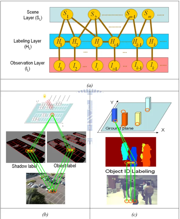
IMAGE. (B) THE SURFACE LAYOUT WITH GREEN, RED, AND BLUE REPRESENTING SUPPORT SURFACES, VERTICAL SURFACES, AND SKY. (C) DETECTION WITHOUT SCENE INFORMATION. THE DETECTION WINDOWS ARE UNIFORMLY DISTRIBUTED IN IMAGE. (D) DETECTION WITH THE PRIOR OF SURFACE LAYOUT. THE DETECTION WINDOWS ARE MAINLY DISTRIBUTED IN THE “VERTICAL” SURFACES. (E) DETECTION WITH THE PRIOR OF DEPTH AND CAMERA VIEWPOINT. THE DETECTION WINDOWS ARE LARGER IN THE NEAR DISTANCE. (F) DETECTION WITH THE PRIOR OF SURFACE LAYOUT, DEPTH AND CAMERA VIEWPOINT. THE DETECTION WINDOWS ARE FEWER AND MORE ACCURATE. (FIGURES COURTESY OF D. HOIEM [56]) ...26 FIG. 14. (A) THE PROPOSED BAYESIAN HIERARCHICAL FRAMEWORK (BHF). (B) BHF FOR

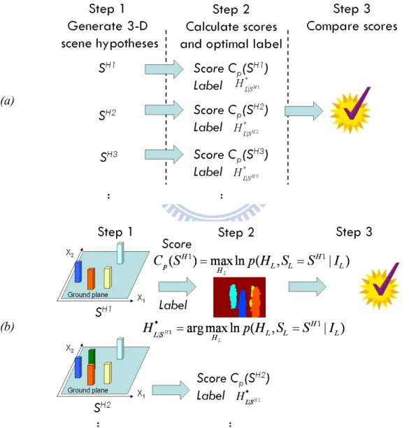
THE VACANT PARKING SPACE DETECTION SYSTEM. (C) BHF FOR THE MULTI-TARGET MULTI-CAMERA SURVEILLANCE SYSTEM. ...29 FIG. 15. EXAMPLES OF SIGM(U) WITHΡ=0.05 AND CTH=100...40 FIG. 16. ILLUSTRATE THE INFERENCE PROCESS OF BHF. (A) A STANDARD INFERENCE

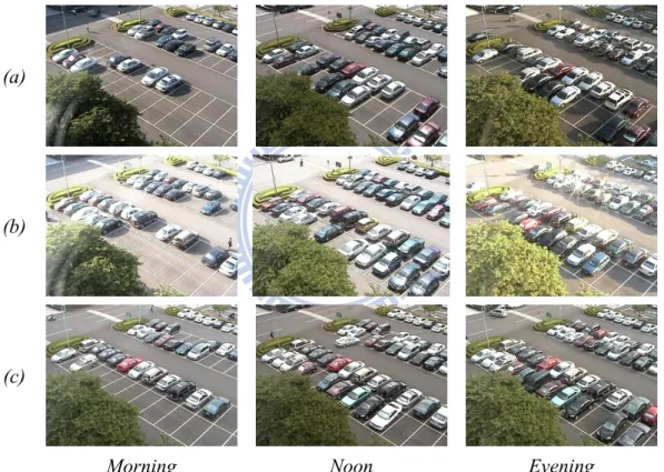
PROCESS. (B) AN EXAMPLE OF BHF INFERENCE PROCESS FOR THE MULTI-TARGET MULTI-CAMERA SURVEILLANCE SYSTEM. ...40 FIG. 17. THE GRAPH SETTING FOR THE GRAPH CUTS ALGORITHM...43 FIG. 18. IMAGE SHOTS OF A PARKING LOT. (A) CAPTURED IN A NORMAL DAY. (B)

CAPTURED IN A DAY WITH STRONG SUNLIGHT. (C) CAPTURED IN A CLOUDY DAY. ..47 FIG. 19. THE CONCEPT OF BAYESIAN HIERARCHICAL FRAMEWORK FOR VACANT SPACE

DETECTION...52 FIG. 20. ILLUSTRATION OF THE 3-LAYER BHF FOR VACANT SPACE DETECTION...53 FIG. 21. (A) A 3-D CAR MODEL. (B) EXPECTED CAR LABELING MAP OF A PARKED CAR.

(C)EXPECTED CAR LABELING OF ALL PARKED CARS. (D) EXPECTED GROUND LABELING OF ALL PARKED CARS. ...57 FIG. 22. (A) SHADOW FORMATION. (B) EXPECTED SHADOW LABELING MAP...59 FIG. 23. (A) A 3-D CAR MODEL. (B) EXPECTED CAR LABELING MAP OF A PARKED CAR.

LABELING OF ALL PARKED CARS. ...59 FIG. 24. ILLUSTRATION OF SOLAR MOVEMENT AND SUNLIGHT DIRECTION. ...60 FIG. 25. (A) A PARKING LOT IMAGE WITH THREE MANUALLY SELECTED IMAGE PIXELS,

MARKED IN RED, GREEN, AND BLUE. (B) THE INTENSITY PROFILES (BLUE) OF THE GREEN PIXEL, OVERLAPPED WITH THE FITTED SKYLIGHT PROFILE (GREEN) AND THE FITTED SKYLIGHT+SUNLIGHT PROFILE (RED)...62 FIG. 26. THE COLOR DISTRIBUTIONS (A) OF SHADOWED GROUND PIXELS, (B) OF

UN-SHADOWED GROUND PIXELS, (C) OF SHADOWED CAR PIXELS, AND (D) OF UN-SHADOWED CAR PIXELS...63 FIG. 27. (A) THE REFERENCE GROUND PATCH (RED) AND THE GROUND PATCHES (PINK)

FOR THE LEARNING OF GROUND REFLECTANCE FUNCTION. (B) THE CAR PATCHES (PINK) FOR THE LEARNING OF CAR REFLECTANCE FUNCTION...67 FIG. 28. ILLUSTRATION OF PARKING SPACE STATUS INFERENCE...71 FIG. 29. COMPARISON OF CAR PIXEL LABELING. (A) TEST IMAGES. (B) REGIONS LABELED

AS CAR PIXELS BASED ON [13]. (C) REGIONS LABELED AS CAR PIXELS BASED ON THE PROPOSED METHOD. ...78 FIG. 30. COMPARISONS OF GROUND PIXEL LABELING. (A) TEST IMAGES. (B) REGIONS

LABELED AS GROUND PIXELS BASED ON [11]. (C) REGIONS LABELED AS GROUND PIXELS BASED ON OUR METHOD. ...78 FIG. 31. THE DETECTION AND LABELING RESULTS AT THREE DIFFERENT TIME INSTANTS.

FOR EACH CASE, THE IMAGES FROM THE TOP ARE THE TEST IMAGE, THE CAR LABELING WITHOUT SCENE KNOWLEDGE, THE CAR LABELING WITH SCENE KNOWLEDGE, THE SHADOW LABELING WITHOUT SCENE KNOWLEDGE, AND THE SHADOW LABELING WITH SCENE KNOWLEDGE. ...79 FIG. 32. THE RECEIVER OPERATING CHARACTERISTIC (ROC) CURVES OF OUR METHOD,

HUANG’S METHOD [46], WU’S METHOD [77], AND DAN’S METHOD [76], WITH THE VALUES OF THE AREA UNDER ROC (AUC) FOR (A)“DAY 1” (B)“DAY 2”, AND (C)“DAY 3” IMAGE SEQUENCES. ...81 FIG. 33. THE PROPOSED DETECTION AND LABELING RESULTS AT THREE DIFFERENT TIME

INSTANTS IN ANOTHER PARKING SPACE. FOR EACH CASE, THE IMAGES FROM THE LEFT ARE THE TEST IMAGE, THE PARKING SPACE DETECTION RESULTS, AND THE CAR LABELING RESULTS. ...83 FIG. 34. SYSTEM FLOW OF THE PROPOSED SYSTEM. ...92 FIG. 35. (A) VISUAL HULL CONSTRUCTED FROM THE FOREGROUND IMAGES OF TWO

CAMERA VIEWS. (B) THE VOXEL HISTOGRAM BASED ON THE VISUAL HULL IN (A). (C) VISUAL HULL CONSTRUCTED FROM FRAGMENTED FOREGROUND IMAGES. (D) THE VOXEL HISTOGRAM BASED ON THE VISUAL HULL IN (C). (E) THE PROPOSED PILLAR MODEL IN THE 3-D SPACE. (F) THE ESTIMATED TDP DISTRIBUTION BASED ON THE

FOREGROUND IMAGES IN (E). (THE RED BAR IN (B)(D)(F) REPRESENTS THE TRUE TARGET POSITION.)...95 FIG. 36. (A) THE TDP OF FOUR MOVING TARGETS IN THE SURVEILLANCE ZONE...97 FIG. 37. AN ILLUSTRATION OF THE GHOST PROBLEM WHEN TRYING TO RECONSTRUCT A

3-D SCENE BASED ON TWO CAMERA VIEWS. ...99 FIG. 38. (A) AN EXAMPLE OF TDP DISTRIBUTION FUSED FROM FOUR CAMERA VIEWS..101 FIG. 39. (A) THE SCENE LAYER IN FIGURE 36 AND TWO OF THE FOUR CAMERA VIEWS. (B)

THE COMBINATION {S1, S2, S3, S4, S5}={1,0,1,1,1} AND THE EXPECTED FOREGROUND IMAGES OVERLAID WITH THE DETECTED FOREGROUND IMAGES. (C) THE COMBINATION {1,1,1,1,1} AND THE EXPECTED FOREGROUND IMAGES OVERLAID WITH THE DETECTED FOREGROUND IMAGES...103 FIG. 40. EXAMPLES OF P(HI(M,N) = TK |S) ...106 FIG. 41. ILLUSTRATION OF THE LABELING RESULTS. (A) TWO CAMERA VIEWS. (B)

WITHOUT AND (C) WITH TARGET MODEL REFINEMENT... 111 FIG. 42. ONE EXPERIMENT RESULT OF OUR LAB SEQUENCE. (A) FOUR CAMERA VIEWS. (B)

FOREGROUND DETECTION IMAGES. (C) TDP DISTRIBUTION. (D) THE VOXEL HISTOGRAM BASED ON THE VISUAL HULL. (E) BIRD-EYE VIEW OF TARGET LOCATION. (F) LABELING AND CORRESPONDENCE OF TARGETS IN PSEUDO-COLOR...116 FIG. 43. ONE EXPERIMENT RESULT OF THE M2TRACKER SEQUENCE. (A) FOUR CAMERA

VIEWS. (B) FOREGROUND DETECTION IMAGES. (C) TDP DISTRIBUTION. (D) THE VOXEL HISTOGRAM BASED ON THE VISUAL HULL. (E) BIRD-EYE VIEW OF TARGET LOCATION. (F) LABELING AND CORRESPONDENCE OF TARGETS IN PSEUDO-COLOR. ...117 FIG. 44. ONE EXPERIMENT RESULT OF THE FLEURET’S SEQUENCE. (A) FOUR CAMERA

VIEWS. (B) FOREGROUND DETECTION IMAGES. (C) TDP DISTRIBUTION. (D) THE VOXEL HISTOGRAM BASED ON THE VISUAL HULL. (E) BIRD-EYE VIEW OF TARGET LOCATION. (F) LABELING AND CORRESPONDENCE OF TARGETS IN PSEUDO-COLOR. ...118 FIG. 45. THE MEAN DEVIATION PER FRAME FOR THE FLEURET’S DATASET. ...119 FIG. 46. ONE EXAMPLE OF EXTENDED SURVEILLANCE ZONE. (A) FOUR CAMERA VIEWS.

(B) THE TDP DISTRIBUTION. (C) BIRD-EYE VIEW OF TARGET LOCATION. ...120 FIG. 47. A COMPARISON OF THE MEAN DEVIATION OF EACH FRAME OVER THE

M2TRACKER DATASET. ...121 FIG. 48. THE DISTRIBUTIONS OF THE NUMBER OF DETECTED TARGET PER FRAME FOR THE

5-PERSON LAB DATASET. (A) RESULTS WITHOUT GHOST REMOVAL. (B) RESULTS WITH GHOST REMOVAL...123 FIG. 49. MULTI-TARGET TRACKING RESULTS (A) M2TRACKER DATASET (4 PERSON). (B)

List of Notations

______________________________________________

BHF Bayesian hierarchical framework IL Observation layer of BHF

HL Hidden labeling layer of BHF

SL Scene layer of BHF

*_, *

L L

H S The optimal solution pair of image content labeling and the 3-D scene parameters

p(SL) The prior knowledge of the 3-D scene statuses

p(HL|SL) 3-D scene model representing the object-level

constraints from scene layer

p(IL|HL) The data constraints from image observation

ED[IL(m,n),HL(m,n)] Classification energy model

EA[IL(m,n),HL(m,n);Np] Adjacency energy model

Np Neighborhood around (m,n)

GS(U) Adaptive function for preserving the discontinuity

Sigm(U) Logistic sigmoid function (m,n) Pixel coordinates

S and US Shadowed label and unshadowed label Ns Number of parking spaces

hO(m,n) Object label at (m,n) hL_{(m,n) Light label at (m,n)}

Ci(m,n) Expected car labeling map at (m,n) given the ith parking

space being occupied

Gi(m,n) Expected ground labeling map at (m,n) given the ith

parking space being occupied

Si(m,n) Expected shadow labeling map at (m,n) given the ith

parking space being occupied

US i(m,n) Expected non-shadow labeling map at (m,n) given the

ith parking space is occupied

IRGB RGB color features of a pixel

N R G B

I Normalized IRGB

R A 3×3 matrix depending on surface reflectance

I A vector depending on illumination

(DX(t),DY(t),DZ(t))T The direction of sunlight

G(X) Target Detection Probability (TDP) Fi Foreground detection result of the ith camera view

Mi Projection image on the ith camera view

Ωi Normalized overlapping area between Fi and Mi

k

μ Mean vector of the kth cluster

k

C Covariance matrix of the kth cluster

p(R) Probability density function of target width p(H) Probability density function of target height

CHAPTER 1

Introduction

______________________________________________

1.1

Overview

Recently, computer vision technology for video surveillance applications has made tremendous progress. Using an intelligent surveillance system to manage parking lots or to monitor security zones is becoming practical. To add more values to existing surveillance systems, various kinds of vision-based intelligent functionalities have been explosively proposed. For example, some algorithms provide user-friendly ways to help operators in the control room to monitor tens of, or even hundreds of, cameras; while a few others provide the capability to automatically detect unusual events in the surveillance zone. These vision-based algorithms may be roughly classified into single-camera based methods and multi-camera based methods. Among those methods, object detection and object labeling are two essential processes for subsequent analyses, like behavior modeling and scene modeling. Object detection, such as face detection and vehicle detection, is an object-level classification that tells

whether and where a specific object is inside an image. On the other hand, object labeling is an identity-level (ID-level) classification that determines the identity of each object region in the image. An example of human detection and human identity labeling is shown in Fig. 1. Even though it seems very easy and straightforward for human eyes to perform object detection and labeling, a robust computational algorithm for these two operations is actually not trivial at all.

(a) (b) (c) Fig. 1. An example of human detection and human identity labeling. (a) Test image. (b) Human

detection result. (c) Human labeling result, with different colors indicating different persons.

For a single camera system, the captured 2-D image lacks the depth information and the detection of moving targets usually suffers from the occlusion problem, which makes it difficult to correctly label or segment connective targets. To deal with occlusion, some methods adopt multi-camera approaches. Even though the cross reference of multiple camera views may ease the occlusion problem and provide a more reliable way for object detection and labeling, the object correspondence among multiple cameras may become another thorny problem.

On the other hand, to detect foreground objects, the appearance ambiguity between the foreground objects and the surrounding background is a challenging issue that may fail many widely-used object detection algorithms. For example, some background subtraction algorithms, like [1][2], focus mainly on the modeling of background information. These algorithms work pretty well for scenes with stationary

background. However, they may detect incomplete foreground regions while the appearance of foreground objects happens to be similar to that of the background. To overcome this appearance ambiguity problem, simply relying on pixel-level image data would not be enough. Some other information, such as region-level messages and object-level messages, should be taken into consideration.

Besides occlusion and appearance ambiguity, the perspective distortion in 2-D images is also a challenging issue. An object far away from the camera and an object close to the camera would have quite different scales and shapes in the camera views. To overcome the perspective effect, some researches focused on invariant feature descriptors. In their approaches, they detect reliable feature points first and design appropriate feature descriptors for object classification. For example, difference of Gaussian (DoG) [3] and Harris-Laplace [4] operators are popular feature extraction operators. The SIFT (Scale Invariant Feature Transform) [5] descriptor is another widely-used operator that is invariant to illumination variation and affine transformation. Even though these operators perform quite well in detecting prominent features, they are still incapable of handling object labeling in complicated scenes.

Shadow effect and lighting variations are another two troublesome issues that degrade the robustness of present surveillance systems. Plentiful works have been proposed to solve these two problems. For example, Finlayson et al. [6] proposed an entropy minimization method to extract from an image the intrinsic image that is shadow-free. Matsushita et al. [7] proposed an illumination normalization method based on an off-line learned eigenspace to eliminate shadows. On the other hand, a few methods have been proposed to maintain reliable color appearance under varying illumination conditions. A review of these color constancy algorithms could be found in [8]. Moreover, in the last decade, the Bayesian approach and some learning-based

methods for color constancy have gotten great attention. A complete survey of Bayesian color constancy methods could be found in [9].

To overcome these aforementioned problems, like occlusion, appearance ambiguity, perspective effect, shadow effect, and lighting variations, we found most existing methods rely more on image observation but less on 3-D scene knowledge. In this dissertation, we focus on the inclusion of 3-D scene knowledge in object detection and object labeling. In our study, we found the usage of 3-D knowledge could be very helpful in handling these complicated issues. Moreover, from the aspect of system functionality, an important role of a practical surveillance system is to dynamically reveal the 3-D status of the surveillance zone. To achieve this functionality, a major task of an intelligent surveillance system would be to automatically infer the unknown 3-D status based on the observed images. In this dissertation, we propose a Bayesian hierarchical framework to realize the integration of 2-D image information and 3-D scene model in a unified and efficient manner for scene inference. The optimal inference of BHF provides a systematic way to resolve the image labeling problem and to find out the 3-D scene unknowns simultaneously. We also apply the framework to two real applications of video surveillance. By using the hierarchical framework to represent the image generation model in a probabilistic manner, our systems can systematically integrate useful information from pixel level, region level, and object level to achieve semantic inference of the 3-D environments.

1.2

Contribution

In this dissertation, by using a parametric form to represent the 3-D scene model with unknown variables, we propose a unified framework, named as Bayesian hierarchical framework (BHF), to accomplish object detection, object labeling, and

to handle these aforementioned issues, like occlusion, appearance ambiguity, perspective effect, shadow effect, and lighting variations. Actually, under the BHF framework, occlusion effect, perspective effect, and shadow effect may even provide useful clues to support 3-D scene inference.

Moreover, the proposed BHF framework has been applied to two video surveillance systems: a vacant parking space detection system and a multi-camera surveillance system. In the vacant parking space detection system, the challenges come from dramatic luminance variations, shadow effect, perspective distortion, and the inter-occlusion among vehicles. With the proposed BHF, those challenging issues can be well modeled in a systematic way and can be effectively handled. Experimental results over a few outdoor parking lot videos show that the proposed framework can systematically detect vacant parking spaces, efficiently label ground and car regions, precisely locate shadowed regions, and effectively handle luminance variations. On the other hand, in the application of multi-target detection and tracking over a multi-camera system, the challenges come from the unknown target number, the inter-occlusion among targets, and the ghost effect caused by geometric ambiguity. Similarly, with the proposed BHF, the target labeling, target correspondence, and ghost removal are regarded as a unified optimal problem subject to 3-D scene priors, target priors, and image observations. Experimental results show that the proposed system can systematically determine the target number, efficiently label and correspond moving targets, precisely locate their 3-D locations, and effectively tackle the ghost problem.

1.3

Organization

The following chapters of this dissertation are organized as follows.

‹ In Chapter 2, we introduce various kinds of messages that have been commonly used for image analysis and scene modeling in video surveillance. Based on the coverage of the information, we classify these messages as pixel-level messages, region-level messages, and object-level messages.

‹ In Chapter 3, we detail the main idea of the proposed BHF framework and how we integrate various kinds of messages under this framework. In this chapter, we first introduce the modeling process in the proposed framework. After that, we depict the inference stage of the BHF framework which determines the optimal estimates of the system unknowns.

‹ In Chapter 4 and Chapter 5, we present the applications of the BHF framework to two different applications. In Chapter 4, we present how we develop a vacant parking space detection system based on the BHF framework. In Chapter 5, we present how we develop a multi-camera surveillance system to perform multi-target detection and tracking. In both systems, we explain how the BHF framework integrates the top-down information from 3-D scene models with the bottom-up message from image observations. The inference procedure of each system is also presented, together with a few experimental results over real scenes to demonstrate the feasibility of the proposed BHF framework.

CHAPTER 2

Backgrounds

______________________________________________

Object detection and object labeling have played an important role in the development of video systems. Some examples, like face detection, human detection, and vehicle detection, have been widely applied to various applications. Right now, a lot of digital cameras can perform automatic face detection while capturing photos. A few intelligent video surveillance systems can count the number of people in the scene based on human detection techniques. For modern intelligent transportation systems, automatic vehicle detection is also prevalent. In the literature, many image analysis works have been proposed to detect or label interested objects. In Section 2.1, we illustrate a few representative algorithms for object detection and labeling. According to the type of information used, these algorithms can be categorized into pixel-level methods, region-level methods, and object-level methods. Since the proposed BHF framework is designed to integrate pixel-level, region-level, and object-level information together, we will briefly review these three types of image analysis methods for object detection and labeling.

On the other hand, with the rapid development of computer vision techniques, scene modeling has attracted more and more attentions. In recent years, the concept of contextual analysis, which physically connects image analysis with scene knowledge, has been intensively studied to achieve improved detection performance. For instance, if we know a car is parked at a certain place and we also know the direction of sunlight, we would expect a shadowed pattern caused by the parked car. This kind of scene knowledge can be helpful in object detection and labeling. Hence, in this dissertation, another focus is to study the way to combine image analysis with the inference of unknown factors in the scene model. In Section 2.2, we will review a few relevant works that discuss the connections between image analysis and 3-D scene modeling.

2.1

Image Analysis Techniques

2.1.1 Pixel-level Methods

In most video surveillance systems, cameras are fixed. This static camera setting relaxes the difficulty of foreground object detection. Ideally, if we collect the color/intensity feature of a pixel over a temporal period, we may find, in most cases, the statistical property of the foreground color/intensity is somewhat different from that of the background color/intensity. Moreover, most of the period, the color/intensity feature at a pixel belongs to the background color/intensity. These two observations are the fundamental assumptions of many pixel-based background subtraction methods. Since background subtraction methods are simple and effective, this background modeling approach has become one of the popular tools in video surveillance applications.

temporal statistical property of every pixel. Based on the learned model, a pixel is classified as either a “background pixel” or a “foreground pixel” based on the current color/intensity observation at that pixel. Besides, the current observation is fed back to update the background model. By on-line learning the statistical property of the background color/intensity, this background modeling method can efficiently extract foreground regions from the background. Currently, several efforts have been proposed for the modeling of time-varying background. Some simpler methods used the 1st order and 2nd order statistics to model the temporal property of a pixel [104]. In these simple approaches, a pixel with its color/intensity feature far away from the mean value is classified as a foreground pixel.

On the other hand, some methods used more complicated parametric forms to model the dynamic statistics of the color/intensity feature at a pixel. Among those methods, the Gaussian mixture model (GMM) has been widely studied and has been proved to be a useful form for background modeling [2]. In principle, the distribution of a pixel value (x) over the temporal (t) direction is formulated as

1 ( ( )) K _i( ) _au( ( ), , )_{i i} i p x t w t g x t μ σ = =

∑

× , (1)

where p(x(t)) is the probability of observing the current pixel value x(t), wi(t) is an

estimate of the weight of the ith Gaussian function gau(.) in the mixture model at Time

t. μi andσi are the mean value and the standard deviation value of the ith Gaussian

in the mixture at Time t. An example of the probability distribution of a pixel with a Gaussian mixture model is shown in Fig. 2.

Fig. 2. The probability distribution of a pixel with Gaussian mixture model [2].

To classify a pixel into either a background pixel or a foreground pixel, Stauffer-Grimson [1] suggested firstly separating the K Gaussian distributions into background Gaussians and foreground Gaussians. Those pixels belonged to background Gaussians are determined as background pixels, and vice versa. To separate the K Gaussian distributions, the ratio wi /σi of each Gaussian distribution

are calculated and is used to rank the K Gaussian distributions from small to large. The first B Gaussian distributions, whose summation of their probability weights exceeds a threshold T, are treated as background Gaussians. This is formulated as

1 arg min( b _i ) b _i B w T = =

∑

> . (2)

On the other hand, the parameter sets {μi,σi ,wi } are dynamically updated over time

to adapt to the environmental variation. By using a recursive filter to approximate the online Expectation-maximization (EM) algorithm [1], the parameter sets are updated based on the following formulation:

( ) (1t ( )) (t t 1) ( ) ( ( ), (t Q x t t 1))

β = −λ β − +λ β − . (3)

Here, β(t) could be any model parameter of {μi,σi ,wi } at Time t, λ(t) is the

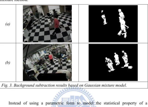
parameterβ(t−1). In Fig. 3, we show the detection results based on the Gaussian mixture method.

(a)

(b)

Fig. 3. Background subtraction results based on Gaussian mixture model.

Instead of using a parametric form to model the statistical property of a background pixel, Elgammal et al. [10] proposed the description of a background model based on non-parametric kernel density estimation. In their method, the pixel-wise statistical property along the temporal direction is modeled by a kernel density function. Given N successive intensity values Bx={x1, x2,…,xN} along a

temporal period at a pixel, they estimate the probability density function (pdf) to be

1 1 ( |_{t x}) N _BW( _{t i}) i p x B K x x N = =

∑

− . (4)

Here, xt represents an intensity value. KBW is the kernel function with bandwidth BW.

By assuming that most of the intensity values inside the observed time period belong to the background, a pixel with a smaller probability value p(xt) is more likely to be a

foreground pixel. To adapt to the environmental variation over time, this algorithm simply shifts the time window to update samples for the estimation of the pdf function.

researchers try to record all possible forms of the background images and then dynamically select the most suitable background image from the stored background image database. Obviously, it would be inefficient to directly store all possible background images in a large database. Hence, Funck et al. [11] assumed that the background images would form a Euklidian subspace within the space formed by all image pixels. By applying the Principal Component Analysis (PCA) technique to calculate the major principal components, any background image could be represented as a linear combination of the derived eigen-backgrounds. With this eigen-background representation, any input image is firstly projected onto the background subspace to find the most matched background image. By subtracting the matched background image from the input image, foreground objects are identified.

Even though the detection of foreground objects based on pixel-level background modeling works pretty well for a scene with stationary background, this approach has difficulty in handling the occasional appearance ambiguity between a foreground object and its surrounding background [12]. When a foreground object happens to have an appearance similar to that of the surrounding background, the background model may not be enough for foreground/background discrimination. Hence, instead of focusing on the background model, some other researchers proposed the learning of the foreground target model. For instance, Tsai et al. [13] developed a probabilistic method to model a pixel-level car model in the chromatic domain. In their method, the RGB color features of many “car” pixels are collected and converted to a new color domain based on the following transformation.

( ) / 3 (2 ) / { / ,( ) / } Z R G B u Z G B Z p Max Z G Z Z B Z = + + = − − = − − . (5)

values of the “car” pixels cluster compactly in the u-p color space. This cluster can be approximated by a Gaussian function:

1 1 1 ( | ) exp( ( ) ( ) ) 2 2 | | t c c c c c c c P x car x m x m π − = − − ∑ − ∑ (6)

where xc= (u, p) is the chromatic feature of a pixel x, mc is the estimated chromatic

mean based on the training set of “car” pixels, and Σc is the estimated chromatic

covariance matrix. Based on the car probability model in (6), the probability of being a “car” pixel at a pixel with the chromatic feature xc can be evaluated.

2.1.2 Region-level Methods

Because of its abilities to adapt to the background variations over time and to cope with multi-modal background distributions, the aforementioned pixel-level modeling has achieved its success in foreground object detection and labeling. Besides, the background modeling approach can handle the situations of new comers and the leave of existing objects. However, in an outdoor scene, occasional camera shaking and the swinging trees caused by strong wind may sometimes seriously degrade the performance of object detection and labeling. In order to improve the performance, some region-level methods have been proposed for image analysis in the literature.

In region-level methods, some researchers extended the concept of GMM to develop new background subtraction methods that incorporate region-level information. For example, Heikkilä et al. [14] tried to model the temporal statistics of a small region to capture the textural information. In [14], local binary patterns were proposed to efficiently extract the texture features of a small region which are invariant to lighting changes. By modeling the dynamic variation of those texture features along the temporal direction, their system outperforms the traditional GMM

background subtraction in an outdoor scene, where the trees were swinging and the camera was shaking. In Fig. 4, we show the detection results based on their method. [14].

Fig. 4. The background subtraction results based on the method proposed by Heikkilä et al. [14]. The first and third rows are the test images. The second and fourth rows are the detection results. (Figures courtesy of Marko Heikkilä [14])

Compared with GMM background modeling, non-parametric kernel based modeling relaxes the constraint of a GMM pdf function and may sometimes provide a more compact match with the true distribution. However, the original non-parametric method is still a pixel-based approach and may suffer from the aforementioned non-stationary effect like camera shaking and swinging trees. In [10], Elgammal et al. suggested an approach that takes into account the background models of neighboring pixels. This is due to the thinking that the intensity value xt at the current pixel may

actually belong to a neighboring pixel at the previous moment. In their approach, they calculated the following probability

( ) max ( | )

N t t y

where y is a pixel belongs to the neighborhood of the target pixel x, xt is the intensity

value at x, and By is the intensity set for the pdf estimation of Pixel y. The distribution

p(xt | By) is estimated by the non-parametric formula in (4). By comparing pN(xt) with

a pre-defined threshold, foreground pixels are determined. A detection result based on the method of [10] is shown in Fig. 5.

(a) (b) (c) Fig. 5. A background subtraction result based on the method of Elgammal et al. [10].

(a) A test image. (b) Per-pixel detection result. (c) Per-pixel detection result with neighboring consideration. (Figures courtesy of A. Elgammal [10] )

Some methods suggested maintaining a region-based foreground model and a background model at the same time for object detection and labeling. A simplest setting is to use a uniform distribution over the feature domain to model the foreground model, as used in [15]. Obviously, the uniform foreground model cannot well capture the foreground property. Hence, Sheikh and Shah [16] expended the original non-parametric kernel density modeling in [10] with some modifications. First, both the foreground model and the background model are dynamically maintained in order to reduce the effect of appearance ambiguity. In their approach, it was assumed that foreground objects tend to have consistent appearance and high spatial correlation in successive frames as long as the video frame rate is high enough. With this assumption, the foreground detection results of the previous frames can be used to establish the foreground model of the current frame. Moreover, in their hybrid

modeling, the background and foreground models compete with each other for a better detection without the need of a manually selected threshold. Second, a new non-parametric kernel density estimation of the probability model over the domain (location) space and the range (color) space is proposed. Rather than modeling the color space only, the integration of the color space and the location space makes it easier to handle non-stationary background in an outdoor scene. In their method, by combining the spatial location x and the pixel color values xrgb into a random vector

d =(x, xrgb), the joint domain-range probability is defined as

1 1 ( | ) N ( i) C BW C i p d d d N = φ Ω =

∑

− . (8)

Here, ΩC={d ,1_C d ,…,_C2 d } is the training set with N domain-range training data of _CN

some class C. In [16], the class C could be foreground (CF) or background (CB). φBW

is the domain-range kernel function with bandwidth BW. While calculating the class probability of a pixel x, ΩC directly embedded the information from neighboring

pixels to contribute the support of the class C. With this design, the non-stationary statistical properties caused by winds or other factors can be overcome.

In some surveillance systems, the video frame rate is low and unstable due to the limited transmission bandwidth or the limited storage. In this kind of surveillance systems, the temporal persistence property required in [16] becomes unreliable. This fact makes foreground modeling difficult. One possible way to model the foreground model would be to exploit the region-level information in the current image. Based on the spatial statistics of the neighboring regions of a pixel, Benedek et al. proposed a method in [17] to build the foreground model of that pixel. They assumed a foreground pixel shares a similar appearance with the other foreground pixels around it. The procedure of the foreground modeling in [17] is illustrated in Fig. 6. To model p(X |S), the foreground probability of a pixel S with the color intensity X , a

manually-defined window VS centered at S is selected as shown in Fig. 6(a). A rough

foreground region F is extracted by background subtraction, as shown in Fig. 6(b). In Fig. 6(c), the intersection region of F and VS is denoted as FS. The histogram of FS is

presented in Fig. 6(d). Those pixels whose intensities are within the range [XS -τ, XS

+τ] are collected for the training of a Gaussian foreground model, as shown in Fig. 6(e). Compared with the uniform foreground model, which gets a likelihood value 2.71 for XS in this example, the spatial statistics based foreground modeling gives a

likelihood value 4.03 for XS which apparently better represents the foreground

property. In Fig. 6(f) and Fig. 6(g), the final detection results are compared based on the uniform foreground model and the spatial statistics based foreground model, respectively. Note that the gray color represents the shadow regions.

Fig. 6. The procedure for the foreground modeling in [17] based on the spatial statistics. (Figures courtesy of Cs. Benedek [17])

Another kind of region-level information is the expansion of spatial similarity. Statistically, adjacent points tend to belong to the same class, especially when the adjacent points share similar appearance. This property is sometimes named the “smooth constraint” of neighboring regions in the literature. To consider spatial similarity while doing image analysis, a popular way is to adopt Markov random field (MRF) model [18][19][20]. In MRF, the smooth constraint is modeled by the clique

potential among neighboring sites. Unlike many previous works which directly assign a suitable class to a pixel, the clique potential only requires the labels of neighboring pixels to fulfill the smooth constraint. Hence, a typical form of MRF usually involves an extra constraint (the data term), which defines the cost of assigning different labels for a pixel, to cooperate with the clique potential. By combining the data term and smoothness term, the MRF provides a flexible framework to integrate pixel-level information and region-level information for image analysis.

2.1.3 Object-level Methods

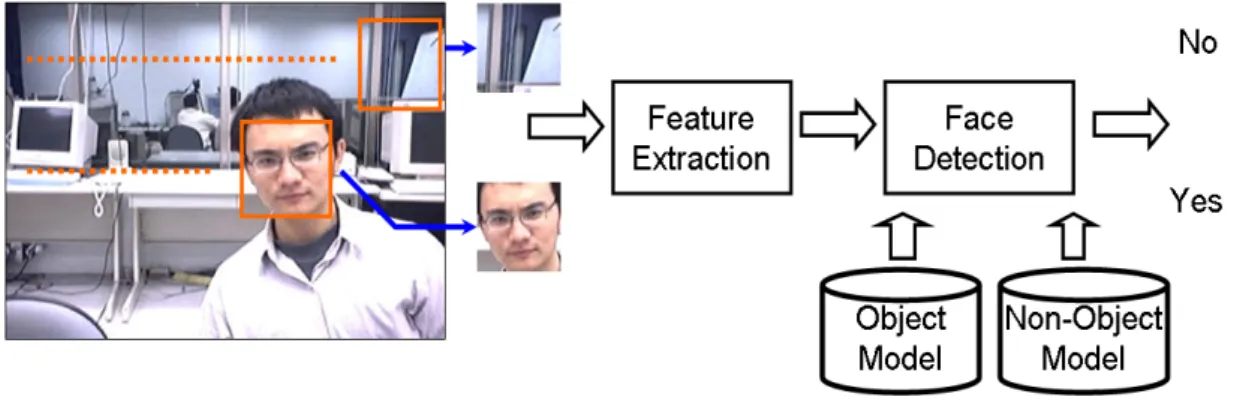
Instead of using pixel-level information to classify local pixels or using region-level information to group neighboring pixels through the use of MRF technique or some other grouping techniques like connected component analysis [23], a few other methods suggest to directly learn the unique object-level property of an object class for detection and labeling. Once the properties of an object class are well learned and modeled, a popular way to detect the interested target is to scan through the image by using a sliding window, as shown in Fig. 7. The discriminative properties of an object class are used to verify whether a target is inside the sliding window. Instead of merging local information to reach the final decision, those object-level methods use the object-level information as a whole for detection and labeling. A typical face detection procedure is illustrated in Fig. 7 as an example. A test window is first selected and the object features inside the window are calculated. By comparing the object features with respect to the object model and the non-object model, we decide whether an object could be found inside the window.

A crucial step for object-level detection is the extraction of object-level information. A systematic way to find the discriminative features of an object class is

process, the object-level information, usually named as trained object model, is extracted and used for the detection task.

Fig. 7. A typical object-based detection procedure with sliding window. Here, we use face detection as an example.

Support vector machine (SVM) is a popular technique to train object models in the field of machine learning [24][25]. Given a set of training examples composed of positive examples and negative examples, the main operation of SVM is to search an optimal hyperplane that separates positive examples from negative examples with a maximum margin. The optimal hyperplane could be expressed as

( ) T ( )

o o

f x =w φ x + . (9) b

In (9), xo is the features calculated from an image patch (window). (.)φ is anonlinear

mapping function to map the input features into a higher dimensional space H. (w,b)

are the major parameters controlling the direction and shift of a hyperplane. In SVM, (w,b) are the major factors to learn. They are only determined by the support vectors, which are the borderline training examples in the dataset. Those support vectors represent almost all the information of the training dataset. We may treat these support vectors as the extracted object-level information learned from the SVM training process. The positive support vectors define the object model while the negative support vectors define the non-object model. In Fig. 8, we illustrate the concept of

SVM classification.

Fig. 8. Illustration of SVM classification with a hyperplane that separates positive examples (“+”s) from negative examples (“O”s) with the maximum margin. Support vectors are parts of the training examples that lie on the boundary.

In the literature, the feature xo in (9) calculated from an image window has

played an important role in the performance of object detection. In general, a good feature is required to be invariant to illumination variations. Recently, a few features are commonly used, including the cascaded raw color pixel over the window [26], the wavelet-like features [27], and the histogram of oriented gradients (HOG) [28].

In object detection, a major difficulty is the need to deal with various kinds of variations, like appearance variation or shape variation. In a practice system, variations mainly come from intra-class difference, environmental illumination, and object deformation. To achieve robust object detection, a sophisticated but flexible object model is needed. However, an object-level model learned from the typical SVM procedure is more like to be a rigid template. While dealing with non-rigid object detection, the typical SVM-based object model may not be a proper solution. To overcome non-rigid deformation, the pictorial structure framework was first proposed in [29] and then extended by [30][31][32]. As illustrated in Fig. 9, the pictorial structure framework represents an object model by a set of parts that are

located in a deformable manner. Each part captures some local appearance properties of an object. Deformable models is also learned to characterize the spring-like connections between each pair of individual parts.

Fig. 9. The pictorial structure framework proposed by Fischler and Elschlager [29].

To learn a part-based object model based on a typical training dataset, where the positive examples are only selected by bounding boxes without any training information of the object parts, the SVM learning procedure would not be suitable. This is because the locations of object parts in each positive example are latent and unknown for training. In [32], Felzenszwalb et al. adopted the latent SVM [33] to handle latent factors. In latent SVM, the first step of the learning procedure is to maximize over latent part locations to find out the optimal part locations for each positive example based on a learned object model in the current iteration. The second step is to refine the object model based on the training dataset and the optimal part locations found in Step one. These two steps are iteratively performed until the final object model converges. As an example, we show a human model with its part models and deformable models in Fig. 10(c)(d). Here, HOG is used as the feature in this example. The deformable models allow each part to deviate from a reference location and can adapt to the variation caused by deformation. In Fig. 10(a), a result of human detection shows the deviation of each body part.

(a) (b) (c) (d) Fig. 10. The part-based object detection reported in [32]. (a) A tested image with the

detected human and its parts. (b) The HOG human model. (c) The HOG models of each body parts. (d) The deformable models depicting the possible variation of each part. (Figures courtesy of P. Felzenszwalb [32])

If looking into the SVM learning procedure, we may find the SVM procedure “equally” takes into account the entire local feature space to maximize the margin while minimizing the number of incorrectly classified examples. Hence, the object model learned by the SVM process gives an equal weight to each local property of the object. However, different local area may have different degrees of discriminability. This brings the idea of feature selection while learning an object model. The AdaBoost technique [34][35][36] is a successful method, which incorporates feature selection into object model learning with a unified training procedure. Instead of combining many features with an equal weight like SVM, the AdaBoost procedure selects a few but important features to represent object information and creates a sparse classification rule for object detection.

A main feature of AdaBoost is its ability to select the discriminative features. This is achieved by dynamically adjust the weights of each training sample. However, a typical AdaBoost algorithm does not put too much effort on the combination of local features. On the contrary, SVM method put more effort on the combination of local features through the use of different kernels. Recently, a few research works [37][38]

focus on the integration of AdaBoost algorithm and SVM method. The AdaBoost algorithm is used to select discriminative features for the object detection while the SVM process is used to determine the final classifier by fusing the selected features.

Besides utilizing a learning-based method to obtain object-level information, some previous works directly design the specific target body structure for detection. For instance, human is a very important class for video surveillance systems. Hence, many works have been proposed to design a suitable representation for human detection. Basically, the proposed human model is composed of some simple elements, such as blobs, pillars, ellipses, and cylinders. The conventional human representations include the ellipse model [40], the stick figure model [41], the 2-D contour model [42], and the volumetric model [43]. After the body structure is defined, object detection is accomplished by fitting the target structure model to the image observation. In Fig. 11, we illustrate a few commonly used representations for the human model.

(a)A ellipse human model [40] (b)A stick-figure human model [41]

(c) A 2D contour human model [42] (d) A volumetric human model [43] Fig. 11. Four representation methods for the human model. (Figures courtesy of JK Aggarwal [39])

2.2

Connection between Image Analysis and 3D

Scene Modeling

Besides using pixel-level, region-level, and object-level information for image analysis, another useful clue is to rely on the prior knowledge of 3-D scene. For instance, in a lobby, we would expect a few people walking on the ground plane. Based on this prior knowledge plus an appropriate 3-D human model, object detection may become more stable, as reported in [44] and [45]. On the other hand, for a typical parking lot, we may know the 3-D layout of the parking spaces. Based on this prior knowledge plus suitable 3-D car models, the detection of parked cars may become more robust and reliable [46].

The study of the connection between vision analysis and scene modeling has a long history. In the 19th century, James Gibson [47] proposed that scene surfaces constitute the fundamental of human vision. Human vision can perceive the depth and distance mainly depending on the perception of longitudinal surfaces. Warren [48] also believed that human vision can fully understand the 3-D scene not only based on image observation but also based on lots of visual experiences in daily life. The visual experiences drive human beings to utilize clues, such as horizontal line, shadow, and some familiar objects, to infer the status of the 3-D scene. Moreover, Koenderink et al. [49][50] found that the participants of their experiments could not measure the depth order of two points in the scene unless there is a scene surface connecting these two points. Those findings suggested that physical surfaces provide valuable information for scene interpretation.

In the recent study of video surveillance techniques, an example of utilizing surface information to improve system accuracy is the use of the 3-D prior that human stands on the ground plane [40]. Based on this assumption, Object detection and

tracking become more robust. Moreover, Hoiem et al. [51][52] believed the extraction of the surface layout in an image is a right way to interpret the 3-D scene. Hence, they proposed a learning based method to assign each image pixel a geometric class. To find out the surface layout, Hoiem et al. [52] firstly over-segmented an image observation. Each segmented region was named as a super-pixel. By merging similar super-pixels based on some local features, like color, texture, location and shape, their algorithm generated a large set of segmented regions. The learned surface models were utilized to assign a surface class to each segmented region. Once the surface layout is extracted, Hoiem et al. [53][54] used the surface knowledge to reconstruct 3-D view based on a single image. In Fig. 12., we illustrate the automatic photo pop-up with the help of the extracted surface layout.

(a) (b) (c) (d) Fig. 12. Illustrate the process of automatic photo pop-up [54]. (a) An input image. (b)

The surface layout with green, red, and purple representing support surfaces, vertical surfaces, and sky. (c) One synthesized image view. (d) Another synthesized image view.

(Figures courtesy of D. Hoiem [54])

On the other hand, 3-D depth knowledge and camera viewpoint are also valuable information for object detection. In general, the camera viewpoint is available if the intrinsic and extrinsic parameters of the camera are available. Furthermore, for a practical video surveillance system, the inter-object occlusion would be a challenge issue. If the depth order of objects could be known in advance, it becomes easier to

handle the inter-object occlusion problem. In [55], Sudderth et al. integrated the depth information to achieve high detection performance. In [56], Hoiem et al. proposed to combine the information of surface layout, depth order, and camera viewpoint to support object detection. The results are shown in Fig. 13. By using the scene knowledge, lots of unlikely detection results are removed.

(a) (b) (c)

(d) (e) (f) Fig. 13. Human detection based on scene knowledge [53][56]. (a) An input image. (b)

The surface layout with green, red, and blue representing support surfaces, vertical surfaces, and sky. (c) Detection without scene information. The detection windows are uniformly distributed in image. (d) Detection with the prior of surface layout. The detection windows are mainly distributed in the “vertical” surfaces. (e) Detection with the prior of depth and camera viewpoint. The detection windows are larger in the near distance. (f) Detection with the prior of surface layout, depth and camera viewpoint. The detection windows are fewer and more accurate. (Figures courtesy of D. Hoiem [56])

Some researches tried to estimation the depth map from a single image. Oliva and Torralba [57] found some image local properties, such as naturalness, openness,

roughness, expansion, and ruggedness, are directly relevant to the 3-D depth. By measuring those local properties from a single image, a rough depth map could be estimated. Moreover, Saxena [58] proposed an MRF-based framework to integrate local image properties to infer the depth map. The extracted depth order is then utilized to help image analysis.

On the other hand, instead of using scene knowledge, like scene surfaces or depth order, to help object detection, some researchers began to think in the opposite way. Sudderth et al. [59] suggested that by understanding the relations among multi-targets, the depth information can be derived.

In this dissertation, we study another possibility to combine image analysis and scene modeling in a unified framework. According to the findings of these previous works, image analysis and scene modeling are highly relative and are complementary to each other. However, in a practical video surveillance system, we usually have some unknowns in both 3-D scene model and 2-D image contents. This drives us to propose the Bayesian Hierarchical Framework (BHF) to simultaneously infer the status of 3-D scene model and label objects in the image domain.