股票訂價折現模型-以台灣股票市場為例

國立交通大學

經營管理研究所

碩士論文

股票訂價折現模型-以台灣股票市場為例

Taiwan Stock Valuation with Time-Varying

Discount Factor

研 究 生: 曹家銘

指導教授: 周雨田 教授

Taiwan Stock Valuation with Time-Varying

Discount Factor

研 究 生:曹家銘 Student: Chia-Ming Tsao 指導教授:周雨田 教授 Advisor: Ray Yeutien Chou

國立交通大學

經營管理研究所

碩士論文

A Thesis

Submitted to Institute of Business and Management of

National Chiao Tung University

In Partial Fulfillment of the Requirements

For the Degree of

Master of Business Administration

June 2012

股票訂價折現模型-以台灣股票市場為例

Taiwan Stock Valuation with Time-Varying

Discount Factor

研究生:曹家銘 指導教授:周雨田 教授

國立交通大學經營管理研究所碩士班

中文摘要

有別於 Chow [2] 在假定折現因子為常數的情況下，考慮了現金股利和現金股利 成長率所建立的傳統股票訂價模型，在適應預期的基本假設下，本文嘗試將此非 線性模型，推廣至一個更一般化的股票評價模型。本篇論文包含了四組模型，藉 由將折現因子納入模型中，以及透過不同類型股票的時間序列資料，我們欲探討， 現金股利、現金股利成長率、名目無風險利率以及市場風險溢酬是否對於台灣地 區指數型基金和傳產類股之成份股的股票價格產生影響。本文除了使用指數型基 金的成份股為樣本資料外，更首次將類股資料導入非線性的股利折現模型中。研 究結果顯示：(1) 在我們選擇的三種指數型和八種傳產類股中，只有台灣高股利指 數、食品類、機電類以及金融類股資料在我們使用的一般化股利折現模型中，符 合適應預期的基本假設；(2) 由部分樣本資料不符合適應預期的研究結果，我們可 以推測其個別投資人較不受過去財務訊息所影響；(3) 在我們所討論的成份股中， 我們普遍發現其個別投資人對於股利成長率與股價的的關係存在著悲觀觀點，而 這樣的觀點恰與 Chow [29] 以香港恆生指數為樣本之研究結果不謀而合；(4) 針對 傳統的八大類股而言，由於相似的股利政策和市場風險溢酬，使得僅有機電和建 築類股的股票價格能被模型所解釋；(5) 我們進一步發現，在傳統的股利折現模型 中，水泥窯業、食品以及機電類股之非限制方程式的係數具有相似的現象，儘管 這些類股分屬不同產業，但這樣的結果隱含著這些類股的股價受到相似的因素所 影響; (6) 透過統計檢定方法，我們發現名目無風險利率的期望值以及市場風險溢 酬的期望值對於台灣股票價格具有顯著的影響，同時也說明了考量折現因子後的 一般化股票評價模型更能捕捉台灣地區的股票價格。 關鍵字: 適應預期、非線性折現模型、股票訂價模型、折現因子、市場風險溢酬

Taiwan Stock Valuation with Time-Varying

Discount Factor

Student: Chia-Ming Tsao Advisor: Ray Yeutien Chou

Institute of Business and Management

National Chiao Tung University

Abstract

In contrast with the model of Chow [2], which implied that the logarithm stock price is a linear function of expected log dividends and the expected rate of growth of dividends under the assumption of the adaptive expectation, we have attempted to provide a general approach to estimation of models with stock price in this paper. This research includes four models designed to investigate how dividends, growth rate of dividends, nominal risk-free rates and risk premiums affect individual stock prices by using the different kinds of data for stocks. Following the theoretical framework of Chow [2], our researches use the individual stock of the stock market index as well as the individual stock of the eight major sectors as data in four models. The preliminary findings are: (1) Only the individual stock of TWSE Taiwan Dividends+ Index, Cement & Ceramics, Foods, Electric & Machinery, Construction and Finance sectors are consistent with the assumption of adaptive expectation. (2) The data which are not fit the adaptive expectations may suggest that the investors of these data do not take the historical information into consideration. (3) Furthermore, we discover that the coefficients α for Etdt are practically zero in the data, which are consistent with the

adaptive expectations. Similar to the results of Chow [29], which used the Hang Seng Index, the empirical phenomena suggest that the overall pessimistic view of investors in these data. (4) For individual stock of the eight major sectors, merely the individual stock of the Electric & Machinery and Construction are consistent with the adaptive expectation hypothesis and can be explained by the expected level of log dividends. (5) We further discover that the unrestricted β coefficients are similar in the Cement & Ceramics, Foods, and Electric & Machinery sectors in model 1. This result indicates that behaviors in these sectors are identical. (6) According to the statistical test, we have strong evidence that the expected nominal free-risk rates and expected risk premiums have significant effect to contribute the current pricing. Besides, we find statistical evidence supporting the general model of stock price formation.

Keywords: Adaptive Expectations; Nonlinear Present-Value Model; Stock Valuation Model; Discount Factors; Risk Premiums

誌謝

時光飛逝，很開心順利完成這個人生的階段性任務。人生總是充滿著意外，但 又不得不佩服上天的安排；2009 年的一場運動傷害、一場失敗的告白，不知道是 逃避還是不服輸的個性使然，我把三萬塊的保險理賠金都給了補習班，只有七個 月的時間，我考上交大。進入交大，能認識這麼多優秀的同學、能得到國內最頂 尖教授的指導，甚至是順利的拿到碩士學位，對我來說就好像做了一場夢。首先， 我要感謝我的論文指導教授-周雨田老師，在論文的撰寫上對我的指導和幫助；記 得老師常說，做研究要站在巨人的肩膀才能看得遠，能成為老師的指導學生以及 能與老師在學術議題上有這麼多的討論，都使得學生不論在學術的討論甚至是思 維邏輯上有了很大的成長。同時，也感謝初稿審查委員丁承老師、胡均立老師的 寶貴意見，以及口試委員周恆志教授、楊奕農教授的指教，因為這些老師的幫助， 才使得學生的論文更趨於完整。此外，我要特別感謝經管所的所長-胡均立教授， 對於胡所長的敬業精神以及對學術上的堅持，學生都感到十分的佩服，希望老師 能保重身體，為經管所開創更美好的將來。 感謝這兩年來，給我不斷鼓勵和幫助的夥伴們；謝謝研究室的夥伴，嘉文、煒 婷、小馬、祈妤、Mick、阿拉，能與這麼多優秀的同學共事，是我在經管所感到 最光榮的。另外，我要特別感謝大學時期的學長-紀建文先生，謝謝他在過去我幾 度徬徨、蹉跎的時刻，給我適時的鼓勵和幫助，他是我的偶像，如果沒有他，就 沒有讀交大的我。同時，也祝福他能趕緊與洪茜欣學姐早日結婚，生下美貌智慧 兼具的小寶寶。我還要感謝我的父母，總是支持我的任何決定，或許我的父母沒 有很高的學歷，或許他們時常被瞧不起，但他們對我的百分之百支持，成就了今 天的我，我想，我沒讓你們失望。回首兩年的時光，只能以忙碌來形容，經管所 繁重的課程、撰寫論文的壓力、再加上在外兼課的疲勞，常常讓自己喘不過氣； 幸虧我的身邊還有個溫柔體貼、善解人意的女孩兒-黃怡芬小姐，感謝她這兩年來

容忍我無數次的發脾氣和不貼心，也因為有她精神上的支持和鼓勵，才讓我有動 力不斷的接受挑戰以及順利完成論文。我常覺得，交女朋友就像在買福袋，你永 遠不知道你抽到的是衛生紙還是豪華房車，但我想說，對於我來說，妳就是上天 給我最好的禮物，因此我希望把這篇論文的榮耀獻給妳。我愛妳。 曹家銘 謹誌於 國立交通大學經營管理研究所 中華民國一百零一年八月

Table of Contents

中文摘要 ... ii

Abstract ...iii

誌謝 ... v

Table of Contents ... vii

List of Tables ...viii

List of Figures ... x

1. Introduction ... 1

2. Stock Prices, Dividends, Interest Rates and Risk Premiums ... 7

3. Data and Estimation Results ... 12

4. Comparison with findings for Taiwan Stocks ... 37

5. Conclusion... 47 References ... 49 Appendix A ... 53 Appendix B ... 54 Appendix C ... 55 Appendix D ... 56

List of Tables

Table 1. The individual stock of the TWSE Taiwan 50 Index ... 12

Table 2. The individual stock of the TWSE Taiwan Mid-Cap 100 Index ... 13

Table 3. The individual stock of the TWSE Taiwan Dividend+ Index ... 14

Table 4. Data Information ... 15

Table 5. The beta for TWSE Taiwan 50 Index, 1991-2010... 16

Table 6. The beta for eight major sectors, 1991-2010 ... 17

Table 7. Unit root tests in stock price series ... 19

Table 8. Unit root tests in dividends series ... 20

Table 9. Unit root tests in risk premiums and nominal risk-free rates series ... 21

Table 10. Results in the TWSE Taiwan 50 Index... 22

Table 11. Results in the TWSE Taiwan Mid-Cap 100 Index ... 24

Table 12. Results in the TWSE Taiwan Dividend+ Index ... 26

Table 13. Results in the Cement and Ceramics sector ... 27

Table 14. Results in the Foods sector ... 29

Table 15. Results in the Plastics and Chemicals sector ... 30

Table 16. Results in the Textile sector ... 31

Table 17. Results in the Electric and Machinery sector ... 32

Table 18. Results in the Construction sector ... 34

Table 19. Results in the Finance sector ... 35

Table 20. Results in the Paper sector ... 36

Table 21. The data are consistent with the adaptive expectations ... 38

Table 22. The sum of squared residuals of the unrestricted linear regression (5) and ... the restricted linear regression (6) ... 40

Table 24. The sum of squared residuals of the unrestricted linear ...

regression (10) and (12) ... 42

Table 25. The results of F-test by testing the unrestricted linear ... regression (10) and (12) ... 43

Table 26. Results in the market stock index ... 44

Table 27. Four of eight sectors consist with the adaptive expectations in model 1 ... 45

List of Figures

Figure 1. The variance of market return in Taiwan, 1991-2010... 17 Figure 2. One-year deposit rates series in Taiwan, 1991-2010 ... 18

1. Introduction

What are the reasons that cause stock price fluctuation? What factors determine the individual stock price? The relationship between stock prices and the fundamental factors has long been the subject of both theoretical and empirical research in financial economics. Studies by Cutler, Poterba, and Summers [1], have claimed that the variation in aggregate stock price can be attributed to various types of economic news. A standard approach to examine stock price is the present-value model; this fundamental valuation formula implies the stock price is the expected present discount value of future dividend streams.

The present-value model was first used in the stock price determination by Chow [2]. It was based on the model that stated the price of a stock at the beginning of time t was the sum of the expected discounted values of all of its future dividends. In other words, the model of Chow [2] assumed that the logarithm of the price of a stock is a linear function of the expected current log dividend and the expected rate of growth of dividends. Since future dividends were uncertain, Chow proposed to summarize by the expected level dividends and expected growth rate under adaptive expectations. The fundamental valuation formula became nonlinear function of the four parameters.

Furthermore, the empirical research of the nonlinear present-value model was widely used in financial economics since 1958. Michael [3] first used nonlinear present-value model in labor migration and urban unemployment. Michael assumed that the percentage change in the urban labor force was governed by the differential between the discounted streams of expected urban and expected rural real income. Michael and Eduardo [4] used the model for the evaluation natural resource investment projects. The model suggested that the cash flow stream was then equal to the current value of the replicating portfolio. Hamilton and Flavin [5] used the nonlinear present-value model in

Government Deficits. The research investigated whether the historical data provided a basis for expecting a violation of the present-value borrowing constraint. The results provided the proposition that in order to be able to issue interest-bearing debt, the government must promise to balance its budget in expected present-value terms. Lloyd [6] used the nonlinear present-value model to discuss the land price. This paper presented the relationship between land prices and cash rents derived from an encompassing present value framework.

Patricia [7] focused on the estimation of future profitability as the fundamental determinant of firm value. The model indicated that book value and earnings have distinct roles. The price earnings ratio (P/E) was a function of expected changes in future profitability, and the price book ratio (P/B) was a function of the expected level of future profitability. The model predicted that P/B should correlate positively with future return on book value, and that P/E should correlate positively with growth in earnings. Liu [8] used a nonlinear present-value model that allows for a time-varying expected discount rate in conjunction with a VAR process to decompose real-estate risk. The study indicated that cash-flow risk was found to result in a weaker mean reversion process for real estate relative to stocks. Geltner [9] provided an improved present-value model, taking account of the predictability of property returns, was described and found to track or the traditional present-value model with constant expected returns. Analysis in this paper suggested that most of the changes in commercial property market values have been due to changes in expected returns, rather than changes in expected future operating cash flows.

For stock price volatility, Yuhn [10] aimed to an alternative approach based on a cointegrating regression model for the present value relation. Different from the Campbell and Shiller [11], which demonstrated a linear cointegration between stock prices and dividends, this study lied in its distinction between linear and nonlinear

cointegration. The results indicated that a linear cointegration was not appropriate for investigating stock price volatility and a non-linear representation of cointegration was developed. Duffie and Singleton [12] developed a multi-factor econometric model of the term structure of interest-rate swap yields. The model showed that the fixed payment rate of a swap, assuming that the floating rate was London Interbank Offering Rate (LIBOR), can be expressed in terms of present values of net cash flows of the swap contract discounted by a default and liquidity-adjusted instantaneous short rate. In other words, there was an adjusted short rate process that allowed us to develop a term structure model for the swap market in the same way that models have been developed for government yield curves. Kallberg and Liu [13] applied the West and Campbell–Shiller tests of the dividend pricing relation to an index of real estate investment trusts (REITs). Similar to previous research, this research suggested that, for the REIT population, dividend pricing models cannot be rejected. The present-value model was poor predictors of true prices when tested on market indexes.

Talan [14] used the nonlinear present-value model on the current account of durables consumption. Different from the previous studies, assuming that all goods were traded and that aggregate consumption decisions can be closely approximated by a random walk process, Talan extended these models by explicitly introducing durables and nontrade goods into an intertemporal model of the current account. Since forecasts derived from standard intertemporal current account (ICA) models generally failed to match the volatility of actual current accounts, Gruber [15] offered a solution to the ‘‘excess volatility’’ problem of standard ICA models by incorporating consumption habits into the standard model. The model showed that significant habit formation implies increased current account volatility, as sluggishness was introduced into the consumption adjustment process that followed income shocks. According to Hall [16], which pointed out that because stock price predicted the future state of the economy, it

predicted consumption. Yoshihiro [17] used the present-value model on the current account and stock returns. The model assumed that consumption depended on permanent income, and the empirical finding indicated that a representative agent smoothes consumption based on stock market information.

Recent stock price movements had led to a re-examination of the present-value model. Several studies of asset pricing have challenged the views that stock price were attributed to future dividend streams. Bansal and Lundblad [18] and Bansal and Yaron [19] argued that dividends may be potentially poor instruments because dividends were often manipulated or smoothed. Shiller [20] had shown evidence that stock returns were fluctuating too much to be explained by shocks to future cash flows or plausible variations in future discount rates, argued for other sources of movement in asset prices. Shiller [21] also claimed a change in the volatility of either future cash flows or discount rates caused a change in the volatility of stock returns in present-value models. In addition, Shiller showed the evidence that stock market volatility cannot be explained by movements in the rational expectation of future dividends and interest rates. Hence, we believe that more than one factor drives the dynamics of cash flows. Grossman and Shiller [22] argued the variability of stock prices can be attributed to information regarding discount factors (i.e., real interest rates), which were in turn related to current and future levels of economic activity. The capital asset pricing model (CAPM) of Sharp [23] implied that the expected return on a risky asset was estimated as the risk free rate plus an expected risk premium. The CAPM implied that the risk of the market portfolio was measured by the variance of its returns, so that the risk premium for the market portfolio increased with the variance of its returns. Further, Merton [24] gave an intertemporal CAPM model which implied a linear relationship between the equity premium and the market return variance.

The empirical validity of the hypothesis of rational expectations and adaptive expectations have been studied since the 1980s. According to Muth [25], under the rational expectations, we equate the subjective expectations in the minds of the

economic agents with the mathematical expectations generated by the econometric

model used by the econometrician. Based on Hicks [26], under the adaptive

expectations, we interpret the subjective expectation in the minds of economic agents and not as a mathematical expectation given the information used by the econometrician. Even though Lovell [27] has shown further evidence that the validity of the rational expectation hypothesis by applying it to the present-value model. Many studies have attempted to test the present-value model under the rational expectation hypothesis and have different results from Lovell [27]. The studies of Campbell and Shiller [11], Fama and French [28], Poterba and Summers [29] and West [30] have found that the rational expectation hypothesis may have some restrictions on the present-value model. These restrictions for the rational expectation hypothesis may suggest that the data was inconsistent with the models. In spite of the skepticism of empirical validity for the rational expectations, the hypothesis of rational expectation still have much interested in financial economics in 1980s.

According to results by Chow and Kwan [31], who used the rational expectations hypothesis and the adaptive expectations hypothesis to discuss the Hong Kong stock prices, the present-value model can explain panel data of prices of individual stock and aggregate time series data on Hong Kong stock price index under the adaptive expectations hypothesis. The result indicated that an argument supporting the rational expectations hypothesis for econometric models was followed from (1) the correctness of the model, and (2) the economic agents having at least as much information as the econometrician building the model. In addition, both Campbell and Shiller [11] and Chow [32] have shown strong statistical evidence that the model is not significant under

rational expectations. The problems arisen from applying the rational expectation hypothesis may be due to the fact that the general investors have no better model to estimate the expected variables. Based on Chow [32], which has provided the strong statistical evidence to support the present-value model under adaptive expectations, we assume the variables of this model, dividends, growth rate of dividends, nominal risk-free rates and risk premiums, following the adaptive expectations hypothesis.

In contrast to the models of Chow [2], we try to build a general model which includes the variables of dividends, growth rate of dividends, nominal risk-free rates, and risk premiums. We still assume the expected dividends grow at a constant rate g, but the restriction of a constant discount rate is removed. Our model implies that the logarithm stock price is a linear function of expected log dividends, expected log rate of growth, expected log nominal risk-free rates, and expected log risk premiums under the assumption of adaptive expectation. According to Merton [24] and [33], we consider a linear relationship between risk premiums and market return variances. To examine if the present-value model is suitable for different kinds of stocks with a new approach, we will be using the individual stock of market index as well as different kinds of industry data to construct the model in our researches. Data in our models is divided into two parts. First, we use individual stock of the stock market index in Taiwan, which including TWSE Taiwan 50 Index, TWSE Taiwan Mid-Cap 100 Index, and TWSE Taiwan Dividend+ Index. Secondly, we also use individual stock of the eight major sectors in Taiwan, which including Cement & Ceramics, Foods, Plastics & Chemicals, Textiles, Electric & Machinery, Construction, Finance and Paper sectors.

The aforementioned analyses focus on two purposes: First, we try to build a general nonlinear present-value model, which consider expected level of dividends, expected rate of growth and expected discount factors. Secondly, by using different kinds of stock data, we would like to know if the present-value model built under the assumption of

adaptive expectation can explain different industries’ stock price. The remainder of the article is organized as follows. Section 2 presents the theoretical framework of individual stock prices given by Chow [2]. We present the data and the estimation result in section 3. In section 4, we compare and discuss the estimation result from four models, which one is the best model to explain the stock prices. The last section provides the conclusion for this paper.

2. Stock Prices, Dividends, Interest Rates and Risk Premiums

Our model of stock price determination can be derived from the present-value model as follows. The present value model is

)

1

(

)

1

(

0 , Π 0    _{ }  







i s t s t f i s i t t t

m

r

D

E

S

Where St is the price of a stock at the beginning of period t, Dt+1 is the forthcoming

dividend during the period t+1. rf,t+s and mt+s are respectively the nominal risk-free rate

and the risk premium at period t+s. Eq. (1) is the familiar fundamental valuation formula which including nominal risk-free rates and risk premiums.

If the expected dividend is assumed to grow constant rate g so that

EtDt+s=(EtDt)(1+g)s, Eq. (1) can therefore be simplified to:

)

2

(

)

1

(

0 , Π 0

g

m

r

D

E

m

r

D

E

S

s t s t t t i s t s t f i s i t t t













     _{ }  

Taking logarithms, gives st = lnSt = ln(EtDt) ln(rt+s+mt+sg) ≒

ln(EtDt)1rt+smt+s+g. Where the value of rt+s + mt+sg have to smaller than one and

all ln(EtDt), rt+s, mt+s, and g have to be estimated.

To extend the model to a general model, we simultaneously consider dividends, rate of growth of dividends, nominal risk-free rates and risk premiums into our model. In model 4, we assume that ln(EtDt) is a linear function of the adaptive expectation of lnDt = dt for the forthcoming period and that the permanent expected growth rate g is a linear function of the adaptive expectation of gt = dt dt-1 for the forthcoming period. The adaptive expectations for the forthcoming period are formed by

Etdt = Et1dt1 + c(dt1Et1dt1) = c[1(1c)L]1dt1

Etgt = Et1gt1 + b(gt1Et1gt1) = b[1(1b)L]1gt1

Etrt = Et1rt1 + e(rt1Et1rt1) = e[1(1e)L]1rt1

Etmt = Et1mt1 + h(mt1Et1mt1) = h[1(1h)L]1mt1 (3)

Where L denotes the lag operators，Ldt = dt1, Lrt = rt1, Lmt = mt1. Under the

assumption of adaptive expectation, the adjustment coefficients c, b, e, and h in the adaptive formation of expected level of log dividends, expected log rate of growth, expected log nominal risk-free rates and expected level of log risk premiums, respectively, must between zero and one. The reason for adjustment coefficient is due to the expected variable become negative, when adjustment coefficient is over than one. As one extreme case, if adjustment coefficient = 0, the model reduces to a naive prediction of no change; alternatively, if adjustment coefficient =1 we continue with the same static forecast as before without revision for current error.

Under our assumption, the present-value model for the logarithm st of stock price at

the beginning of period t becomes

Where the coefficient δ, α, τ, ω, γ are respectively represent expected dividends, expected growth rate, expected nominal risk-free rates, expected risk premiums and constant term. Multiplying Eq.(4) by[1(1c)L][1(1b)L][1(1e)L][1(1h)L] and substituting for Et dt , Et gt , Et rt , and Et mt from Eq.(3), one obtains the following

model for st.

st= β1st1 + β2st2 + β3st3 + β4st4 + β5dt1 + β6dt2 + β7dt3 + β8dt4 + β9dt5 + β10rt1 +

β11rt2 + β12rt3 + β13rt4 + β14mt1 + β15mt2 + β16mt3 + β17mt4 + γ*

(5)

The coefficients from the Eq. (5) are reported in the Appendix A. There are seventeen coefficients(β1,β2,...,β17) in Eq. (5) which derived from eight structural parameters, δ, α,

τ, ω, c, b, e and h. Eq. (5) is a linear functions of the ten coefficients (β1,β2,...,β17) but a

nonlinear function of the eight parameters (δ, α, τ, ω, c, b, e, h). It will be estimated by the method of nonlinear least squares, which minimizes the sum of squared residuals with respect to the eight parameters. The nonlinear restriction will also be tested.

Based on Chow [2], we only consider the logarithm stock price is a linear function of expected of log dividends and the expected rate of growth of dividends in model 1. Under our assumption, the present-value model for the logarithm st of stock price at the

beginning of period t becomes

st = δ．Et dt + α．Et gt + γ (5) Where the coefficient δ, α, γ are respectively represent expected dividends, expected growth rates and constant term. Multiplying Eq. (4) by[1(1c)L][1(1b)L] and substituting for Et dt and Et gt from Eq. (3), one obtains the following model for st.

Where γ*= γ．cb; the coefficients of st : β1 = (2 c b), β2= (1c)(1b); the

coefficients of Etdt: β3 = δc + αb, β4 = δc(1b) αb(2 c), β₅ = αb (1c). Since the five

coefficients(β1,β2,...,β5) in Eq. (6) are derived from four structural parameters, δ, α, c

and b, there is one nonlinear restriction on the coefficients (β1,β2,...,β5). Eq. (6) is a

linear functions of the five coefficients (β1,β2,...,β5) but a nonlinear function of the four

parameters (δ, α, c, b). It will be estimated by the method of nonlinear least squares, which minimizes the sum of squared residuals with respect to the four parameters.

Different from the general model, we respectively consider risk premiums and nominal risk-free rates to our model. In model 2, on the basis of the CAPM model, it implies a linear relationship between risk premiums and market return variances. The CAPM postulates a linear relationship between an asset’s beta (a measure of systematic) and expected return. We will assume that a linear relationship with the market return variance by Merton [8],[17].i.e.

) 7 ( 2 ,m i m i t σ β σ m    ) 8 ( , 2 , m i m i m m i i σ σ ρ σ σ β   

From Eq. (7) and Eq. (8), it will be clear that the higher beta stocks yield may cause higher risk premiums and a higher expected rate of return. Further, we directly calculate

the value of βi and σm2 by using financial data. The risk premiums, m , are t attributed to the value of βi and σm2 , where we consider that m is the sector’s beta t times the variance of market return from different kinds of stock in model 2. Especially, since the beta of the Weighted Price Index of the Taiwan Stock Exchange is used to measure the total market risk in the Stock Exchange, the beta value is a constant figure of one. When we use individual stock of the market index to exam the present-value model, the value of mt will be the variance of market return.

Under our assumption, the present-value model for the logarithm st of stock price at

the beginning of period t becomes

st = δ．Et dt + α．Et gt ω．Et mt + γ (9)

Where the coefficient ω is represent expected risk premiums. Multiplying Eq.(9) by [1(1c)L][1(1b)L][1(1h)L] and substituting for Et dt , Etgt and Et mt from

Eq.(3), one obtains the following model for st.

st= β1st1 + β2st2 + β3st3 + β4dt1 + β5dt2 + β6dt3 + β7dt4

+ β8mt1 + β9mt2 + β10mt3 + γ* (10)

The coefficients from the Eq. (10) are reported in the Appendix B. There are ten coefficients (β1,β2,...,β10) in Eq. (10) which derived from six structural parameters δ, α,

ω, c, b and h.

We directly use the one-year deposit rates to represent nominal risk-free rates in model 3. Under our assumption, the present-value model for the logarithm st of stock

price at the beginning of period t becomes

st = δ．Et dt + α．Et gt τ．Et rt + γ (11)

Where the coefficient τ is represent expected nominal risk-free rates. Multiplying Eq.(12) by[1(1c)L][1(1b)L][1(1e)L] and substituting for Et dt , Etgt and Et rt

from Eq. (3), one obtains the following model for st.

st= β1st1 + β2st2 + β3st3 + β4dt1 + β5dt2 + β6dt3 + β7dt4

+ β8rt1 + β9rt2 + β10rt3 + γ* (12)

The coefficients from the Eq. (12) are reported in the Appendix C. There are ten coefficients (β1,β2,...,β10) in Eq. (12) which derived from six structural parameters δ, α, τ,

3. Data and Estimation Results

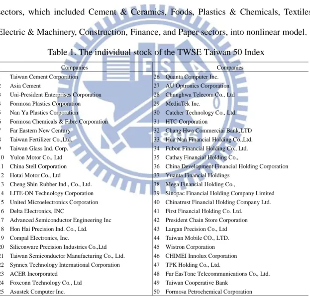
Different from the data of Chow [29], who respectively used individual stocks of the Hang Seng Index, we try to build a general model by different kinds of industrial data for the first time. The data in our models can be divided by two parts. First, similar to the previous models, we focus on individual stock of the stock market index, which included TWSE Taiwan 50 Index, TWSE Taiwan Mid-Cap 100 Index, and TWSE Taiwan Dividend+ Index. Secondly, we try to consider the data of the eight major sectors, which included Cement & Ceramics, Foods, Plastics & Chemicals, Textiles, Electric & Machinery, Construction, Finance, and Paper sectors, into nonlinear model.

Table 1. The individual stock of the TWSE Taiwan 50 Index

Companies Companies

1 Taiwan Cement Corporation 26 Quanta Computer Inc.

2 Asia Cement 27 AU Optronics Corporation

3 Uni-President Enterprises Corporation 28 Chunghwa Telecom Co., Ltd

4 Formosa Plastics Corporation 29 MediaTek Inc.

5 Nan Ya Plastics Corporation 30 Catcher Technology Co., Ltd. 6 Formosa Chemicals & Fibre Corporation 31 HTC Corporation

7 Far Eastern New Century 32 Chang Hwa Commerciai Bank,LTD

8 Taiwan Fertilizer Co.,Ltd. 33 Hua Nan Financial Holding Co.,Ltd.

9 Taiwan Glass Ind. Corp. 34 Fubon Financial Holding Co., Ltd.

10 Yulon Motor Co., Ltd 35 Cathay Financial Holding Co.,

11 China Stell Corporation 36 China Development Financial Holding Corporation

12 Hotai Motor Co., Ltd 37 Yuanta Financial Holdings

13 Cheng Shin Rubber Ind., Co., Ltd. 38 Mega Financial Holding Co.,

14 LITE-ON Technology Corporation 39 Sinopac Financial Holding Company Limited 15 United Microelectronics Corporation 40 Chinatrust Financial Holding Company Ltd.

16 Delta Electronics, INC 41 First Financial Holding Co. Ltd.

17 Advanced Semiconductor Engineering Inc 42 President Chain Store Corporation 18 Hon Hai Precision Ind. Co., Ltd. 43 Largan Precision Co., Ltd

19 Compal Electronics, Inc. 44 Taiwan Mobile CO., LTD.

20 Siliconware Precision Industries Co.,Ltd 45 Wistron Corporation 21 Taiwan Semiconductor Manufacturing Co., Ltd. 46 CHIMEI Innolux Corporation 22 Synnex Technology International Corporation 47 TPK Holding Co., Ltd.

23 ACER Incorporated 48 Far EasTone Telecommunications Co., Ltd.

24 Foxconn Technology Co., Ltd 49 Taiwan Cooperative Bank

25 Asustek Computer Inc. 50 Formosa Petrochemical Corporation

According to TWSE Taiwan 50 Index, similar to the Dow Jones Index for industrial stocks of the New York Stock Exchange, which consists of the fifty blue-chip stocks in the Taiwan Stock Exchange. There are fifty representative stocks of TWSE Taiwan 50

Index listed in Table 1. The market value of TWSE Taiwan 50 Index accounted for 70% of the market.

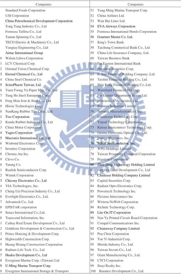
Table 2. The individual stock of the TWSE Taiwan Mid-Cap 100 Index

Companies Companies 1 Standard Foods Corporation 51 Yang Ming Marine Transport Corp. 2 USI Corporation 52 China Airlines Ltd.

3 China Petrochemical Development Corporation 53 Wan Hai Lines Ltd. 4 Tong Yang Industry Co., Ltd 54 EVA Airways Corporation

5 Formosa Taffeta Co., Ltd 55 Formosa International Hotels Corporation 6 Tainan Spinning Co., Ltd 56 Gourmet Master Co. Ltd.

7 TECO Electric & Machinery Co., Ltd 57 King's Town Bank

8 Yungtay Engineering Co., Ltd 58 Taichung Commerical Bank Co., Ltd

9 Airtac Internatinnal Group 59 China Life Insurance Company, Ltd. 10 Walsin Lihwa Corporation 60 Taiwan Business Bank

11 LCY Chemical Corp. 61 Far Eastern International Bank 12 Oriental Union Chemical Corp. 62 President Securities Corp.

13 Eternal Chemical Co., Ltd 63 E. Sun Financial Holding Company ,Ltd.

14 China Steel Chemical Co. 64 Taishin Financial Holding Co., Ltd.

15 ScinoPharm Taiwan, Ltd. 65 Shin Kong Financial Holding Co.,Ltd.

16 Yuen Foong Yu Paper Mfg. Co., Ltd 66 Waterland Financial Holdings 17 Tung Ho Steel Enterprise Corp. 67 Far Eastern Department Stores Ltd. 18 Feng Hsin Iron & Steel Co., Ltd 68 Mercuries & Associates, Ltd. 19 Hiwin Technologies Corp. 69 Ruentex Industries Limited 20 NanKang Rubber Tire Corp., Ltd 70 Novatek Microelectronics Corp.

21 Tsrc Corporation 71 Unimicron Technology Corp.

22 Kenda Rubber Industrial Co., Ltd 72 Tripod Technology Corporation 23 China Motor Corporation 73 Kinsus Interconnect Technology Corp.

24 Yageo Corporation 74 Genius Electronic Optical Co., Ltd.

25 Macronix International Co., Ltd 75 Inotera Memories, Inc. 26 Winbond Electronics Corp. 76 MStar Semiconductor, Inc.

27 Inventec Corporation 77 WPG Holdings Limited

28 Chroma Ate Inc. 78 Taiwan Prosperity Chemical Corporation 29 Clevo Co. 79 Pegatron Corporation

30 Tatung Co. 80 Zhen Ding Technology Holding Limited

31 Realtek Semiconductor Corp 81 Farglory Land Development Co., Ltd 32 Wintek Corporation 82 Chailease Holding Company Limited 33 Chicony Electronics Co., Ltd 83 Capital Securities Corp.

34 VIA Technologies, Inc. 84 Radiant Opto-Electronics Corp. 35 Cheng Uei Precision Industry Co., Ltd 85 Powertech Technology Inc. 36 Everlight Electronics Co., Ltd. 86 Flexium Interconnect Inc 37 Advantech Co., Ltd. 87 Wistron NeWeb Corporation 38 EPISTAR corporation 88 Richtek Technology Corp. 39 Senao International Co.,Ltd. 89 Lite-On IT Corporation

40 Transcend Information, Inc. 90 Nan Ya Printed Circuit Board Corporation 41 Cathay Real Estate Development Co., Ltd 91 Compal Communications Inc.

42 Golddsun Development & Construction Co., Ltd 92 Cleanaway Company Limited

43 Prince Housing & Development Corp. 93 Pou Chen Corporation 44 Highwealth Construction Corp. 94 Ton Yi Industrial Corp. 45 Huang Hsiang Construction Corporation 95 Merida Industry Co., Ltd. 46 Radium Life Tech. Co., Ltd 96 Taiwan Secom Co., Ltd.

47 Huaku Development Co., Ltd 97 Giant Manufacturing Co., Ltd.

48 Evergreen Marine Corp. (Taiwan) Ltd 98 CTCI Corporation

49 U-Ming Marine Transport Corp. 99 Sinyi Realty Inc.

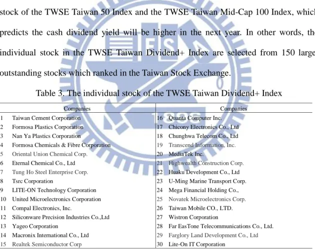
Simultaneously, we also use individual stock of the other stock market index. There are one hundred representative stocks of TWSE Taiwan Mid-Cap 100 Index listed in Table 2. TWSE Taiwan Mid-Cap 100 Index is made up of the 100 large, publicly owned companies in Taiwan, which except for individual stock of the TWSE Taiwan 50 Index. In other words, the individual stock of TWSE Taiwan Mid-Cap 100 Index are ranked from 51th to 150th in the Taiwan Stock Exchange. In comparison with the market value of TWSE Taiwan 50 Index, TWSE Taiwan Mid-Cap 100 Index accounted for 20% of the market. The individual stock of TWSE Taiwan Dividend+ Index are listed in Table 3. TWSE Taiwan Dividend+ Index is composed of the 30 listed companies in individual stock of the TWSE Taiwan 50 Index and the TWSE Taiwan Mid-Cap 100 Index, which predicts the cash dividend yield will be higher in the next year. In other words, the individual stock in the TWSE Taiwan Dividend+ Index are selected from 150 large, outstanding stocks which ranked in the Taiwan Stock Exchange.

Table 3. The individual stock of the TWSE Taiwan Dividend+ Index

Companies Companies

1 Taiwan Cement Corporation 16 Quanta Computer Inc.

2 Formosa Plastics Corporation 17 Chicony Electronics Co., Ltd

3 Nan Ya Plastics Corporation 18 Chunghwa Telecom Co., Ltd

4 Formosa Chemicals & Fibre Corporation 19 Transcend Information, Inc. 5 Oriental Union Chemical Corp. 20 MediaTek Inc.

6 Eternal Chemical Co., Ltd 21 Highwealth Construction Corp.

7 Tung Ho Steel Enterprise Corp. 22 Huaku Development Co., Ltd

8 Tsrc Corporation 23 U-Ming Marine Transport Corp.

9 LITE-ON Technology Corporation 24 Mega Financial Holding Co., 10 United Microelectronics Corporation 25 Novatek Microelectronics Corp.

11 Compal Electronics, Inc. 26 Taiwan Mobile CO., LTD.

12 Siliconware Precision Industries Co.,Ltd 27 Wistron Corporation

13 Yageo Corporation 28 Far EasTone Telecommunications Co., Ltd.

14 Macronix International Co., Ltd 29 Farglory Land Development Co., Ltd 15 Realtek Semiconductor Corp 30 Lite-On IT Corporation

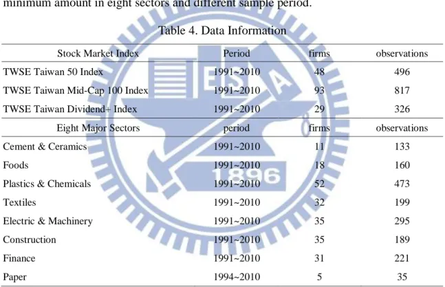
Furthermore, the individual stock of the eight major sectors are reported in the Appendix D. Since different companies have different time to be a listed company and did not issue dividends in cash every year, the total information of the data is listed in Table 4. To fulfill the purpose of researches, which investigate how dividends, growth

rate of dividends, nominal risk-free rates and risk premiums affect individual stock prices, we build the unbalanced panel data. For the stock market index, the date covers a period from 1991 to 2010 and total number of observations respectively are 496, 817 and 326. In the second section, we consider individual stock of the eight major sectors in Taiwan. The eight major sectors we selected in Taiwan Stock Exchange are respectively Cement & Ceramics sector, Foods sector , Plastics & Chemicals sector, Textiles sector, Electric & Machinery sector, Construction sector, Finance sector, and Paper sector. We discover that the samples of individual stock in Paper sector has minimum amount in eight sectors and different sample period.

Table 4. Data Information

Stock Market Index Period firms observations

TWSE Taiwan 50 Index 1991~2010 48 496

TWSE Taiwan Mid-Cap 100 Index 1991~2010 93 817

TWSE Taiwan Dividend+ Index 1991~2010 29 326

Eight Major Sectors period firms observations

Cement & Ceramics 1991~2010 11 133

Foods 1991~2010 18 160

Plastics & Chemicals 1991~2010 52 473

Textiles 1991~2010 32 199

Electric & Machinery 1991~2010 35 295

Construction 1991~2010 35 189

Finance 1991~2010 31 221

Paper 1994~2010 5 35

In this research we will use four models, built upon the assumption of adaptive expectation, to explain the prices of stocks in Taiwan. Following the model of Chow [2], our model only implies that the logarithm stock price is a linear function of expected log dividends, expected log rate of growth in model 1. In regards to data for stock prices, the price of stock was reflected by the market value of the listed company; when a listed company issues cash dividends, the market value of the stock prices will reduce.

For market value of post-dividend stocks, we use the ex-dividend stock prices to build the unbalanced panel data. Consequently, since the data ranges across a time span of 20 years, we will also take the effect of inflation into account. To solve the issue with inflation, we use the GDP deflator (2006 = 100), which is a measurement of the level of prices of all new, domestically produced, final goods and services in an economy, to process the data. To calculate the real stock prices, we will divide the ex-dividend stock prices by the GDP deflator. For dividends data, the GDP deflator is also used to process the data. After the calculations, we build the data called real cash dividends.

Besides, different from Chow [2], we add two discount factors, nominal risk-free rates and risk premiums into our model. The beta for TWSE Taiwan 50 Index is shown in Table 5. We discover that the average beta for individual stocks of the TWSE Taiwan 50 Index is higher in the Global Financial Crisis in 2009. Furthermore, we also note that the average of individual betas is highest than each years, when Asian Financial crisis happened in 1997.

Table 5. The beta for TWSE Taiwan 50 Index, 1991-2010

Table 6 shows descriptive statistics of beta for individual stock of the eight major sectors. The mean beta of Electric & Machinery sector is at the summit in 20 years, which suggests that the individual stock may have higher systematic risk. We also

Year Mean Std. Dev. Year Mean Std. Dev.

1991 0.9391 0.0742 2001 1.0139 0.3039 1992 0.8525 0.2606 2002 0.9499 0.3679 1993 0.8660 0.1467 2003 0.9818 0.2975 1994 0.9523 0.2190 2004 0.9865 0.2707 1995 0.8996 0.1980 2005 0.9825 0.4186 1996 0.9203 0.2055 2006 1.0099 0.3851 1997 1.1597 0.3523 2007 1.0223 0.2591 1998 1.1302 0.3008 2008 1.0454 0.2593 1999 0.9915 0.1899 2009 1.0699 0.2979 2000 0.9425 0.2040 2010 1.0067 0.2837

discover that Construction sector have the highest standard deviation in eight major sectors. This result indicates that the beta of Construction sector may have higher volatility than others.

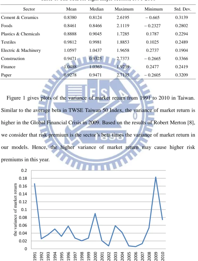
Table 6. The beta for eight major sectors, 1991-2010

Sector Mean Median Maximum Minimum Std. Dev.

Cement & Ceramics 0.8380 0.8124 2.6195 0.665 0.3139

Foods 0.8461 0.8466 2.1119 0.2327 0.2802

Plastics & Chemicals 0.8888 0.9045 1.7285 0.1787 0.2294

Textiles 0.9812 0.9981 1.8853 0.1025 0.2489

Electric & Machinery 1.0597 1.0437 1.9658 0.2737 0.1904

Construction 0.9471 0.9325 2.7373 0.2665 0.3366

Finance 1.0488 1.0363 1.9239 0.2477 0.2419

Paper 0.9278 0.9471 2.7135 0.2605 0.3209

Figure 1 gives plots of the variance of market return from 1991 to 2010 in Taiwan. Similar to the average beta in TWSE Taiwan 50 Index, the variance of market return is higher in the Global Financial Crisis in 2009. Based on the results of Robert Merton [8], we consider that risk premium is the sector’s beta times the variance of market return in our models. Hence, the higher variance of market return may cause higher risk premiums in this year.

Figure 1. The variance of market return in Taiwan, 1991-2010

0 0.02 0.04 0.06 0.08 0.1 0.12 0.14 0.16 0.18 0.2 1991 1992 1993 1994 1995 1996 1997 1998 1999 2000 2001 2002 2003 2004 2005 2006 2007 2008 2009 2010 th e v ar ia n ce o f m ar ke t re tur n

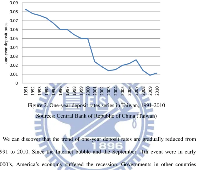
We directly use the one-year deposit rates to represent nominal risk-free rates. Figure 2 gives plots of the one-year deposit rates series from 1991 to 2010 in Taiwan.

Figure 2. One-year deposit rates series in Taiwan, 1991-2010 Sources: Central Bank of Republic of China (Taiwan)

We can discover that the trend of one-year deposit rates are gradually reduced from 1991 to 2010. Since the Internet bubble and the September 11th event were in early 2000’s, America’s economy suffered the recession. Governments in other countries adopt the easy money policy which has the great effect of reducing deposits rates to encourage their domestic economies. From 2000 to 2001, Government in Taiwan rapidly cut down the one-year deposit rates from 5% to 2.41%, which means a 51.8% reduction. We note that one-year deposit rates are maintained around 2% after the year of 2001. Furthermore, when Financial crisis happened in 2009, the one-year deposit rates was reduced under 1%.

0 0.01 0.02 0.03 0.04 0.05 0.06 0.07 0.08 0.09 1991 1992 1993 1994 1995 1996 1997 1998 1999 2000 2001 2002 2003 2004 2005 2006 2007 2008 2009 2010 o n e-y ea r de po si t ra te s

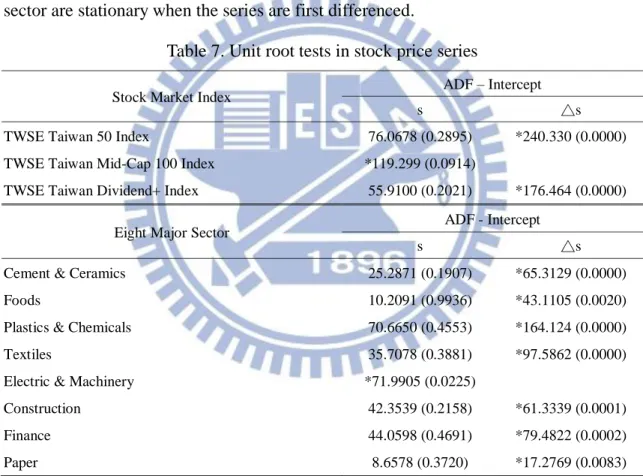
Table 7 contains the results of applying unit root tests to log stock price series. We discover that the unit root hypothesis are rejected in log stock price series of TWSE Taiwan Mid-Cap 100 Index and Electric & Machinery sector. The result indicates that the log stock price series of TWSE Taiwan Mid-Cap 100 Index and Electric & Machinery sector are stationary series. And we note that the stock price series of TWSE Taiwan 50 Index and TWSE Taiwan Dividend+ Index are stationary when the log stock price series are first differenced. Furthermore, the log stock prices series in Cement & Ceramics, Foods, Plastics & Chemicals, Textiles, Construction, Finance and Paper sector are stationary when the series are first differenced.

Table 7. Unit root tests in stock price series

Stock Market Index ADF – Intercept

s △s

TWSE Taiwan 50 Index 76.0678 (0.2895) *240.330 (0.0000)

TWSE Taiwan Mid-Cap 100 Index *119.299 (0.0914)

TWSE Taiwan Dividend+ Index 55.9100 (0.2021) *176.464 (0.0000)

Eight Major Sector ADF - Intercept

s △s

Cement & Ceramics 25.2871 (0.1907) *65.3129 (0.0000)

Foods 10.2091 (0.9936) *43.1105 (0.0020)

Plastics & Chemicals 70.6650 (0.4553) *164.124 (0.0000)

Textiles 35.7078 (0.3881) *97.5862 (0.0000)

Electric & Machinery *71.9905 (0.0225)

Construction 42.3539 (0.2158) *61.3339 (0.0001)

Finance 44.0598 (0.4691) *79.4822 (0.0002)

Paper 8.6578 (0.3720) *17.2769 (0.0083)

NOTE. The null hypothesis is that the series in question contains a unit root in its univariate autoregressive representation. ADF is the regression t-ratio for the autoregressive coefficients to sum to unity-the augmented Dickey-Fuller statistic; * p < 0.1. ; (．): p-value; s: log stock prices; △s: difference of log stock prices

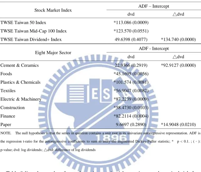
Table 8 contains the results of applying unit root tests to log dividends series. Our conjecture that the log dividends series are stationary in the TWSE Taiwan 50 Index, TWSE Taiwan Mid-Cap 100 Index, Foods, Plastics & Chemicals, Textiles, Electric &

Machinery, Construction, and Finance sector. Furthermore, the log dividends series in TWSE Taiwan Dividend+ Index, Cement & Ceramics Sector and Paper Sector are stationary when the series are first differenced.

Table 8. Unit root tests in dividends series

Stock Market Index ADF – Intercept

dvd △dvd

TWSE Taiwan 50 Index *113.086 (0.0009)

TWSE Taiwan Mid-Cap 100 Index *123.570 (0.0551)

TWSE Taiwan Dividend+ Index 49.6398 (0.4077) *134.740 (0.0000)

Eight Major Sector ADF - Intercept

dvd △dvd

Cement & Ceramics 22.9366 (0.2919) *92.9127 (0.0000)

Foods *45.1695 (0.0056)

Plastics & Chemicals *101.574 (0.0081)

Textiles *56.9047 (0.0082)

Electric & Machinery *87.2239 (0.0009)

Construction *58.4730 (0.0103)

Finance *82.2114 (0.0004)

Paper 9.6697 (0.2890) *14.9048 (0.0210)

NOTE. The null hypothesis is that the series in question contains a unit root in its univariate autoregressive representation. ADF is the regression t-ratio for the autoregressive coefficients to sum to unity-the augmented Dickey-Fuller statistic; * p < 0.1. ; (．): p-value; dvd: log dividends; △dvd: difference of log dividends

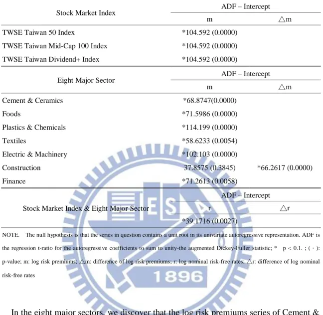
Table 9 lists the results of tests for unit roots in risk premiums and nominal risk-free rates series. Since the beta value, which measured the total market risk, is a constant figure of one in stock market index, the value of risk premiums will be the variance of market return. Hence, the risk premiums series are equal in TWSE Taiwan 50 Index, TWSE Taiwan Mid-Cap 100 Index and TWSE Taiwan Dividend+ Index. We discover that the unit root hypothesis are rejected at the 10% level in log risk premiums series of the Stock Market Index. The result suggests that the log risk premiums series in stock market index are stationary.

Table 9. Unit root tests in risk premiums and nominal risk-free rates series

Stock Market Index ADF – Intercept

m △m

TWSE Taiwan 50 Index *104.592 (0.0000)

TWSE Taiwan Mid-Cap 100 Index *104.592 (0.0000)

TWSE Taiwan Dividend+ Index *104.592 (0.0000)

Eight Major Sector ADF – Intercept

m △m

Cement & Ceramics *68.8747(0.0000)

Foods *71.5986 (0.0000)

Plastics & Chemicals *114.199 (0.0000)

Textiles *58.6233 (0.0054)

Electric & Machinery *102.103 (0.0000)

Construction 37.8575 (0.3845) *66.2617 (0.0000)

Finance *71.2613 (0.0058)

Stock Market Index & Eight Major Sector

ADF – Intercept

r △r

*39.1716 (0.0027)

NOTE. The null hypothesis is that the series in question contains a unit root in its univariate autoregressive representation. ADF is the regression t-ratio for the autoregressive coefficients to sum to unity-the augmented Dickey-Fuller statistic; * p < 0.1. ; (．): p-value; m: log risk premiums; △m: difference of log risk premiums; r: log nominal risk-free rates; △r: difference of log nominal risk-free rates

In the eight major sectors, we discover that the log risk premiums series of Cement & Ceramics, Foods, Plastics & Chemical, Textiles, Electric & Machinery and Finance sectors are stationary. And the unit root hypothesis of log risk premiums series in Construction sector can be rejected at the 10% level when the series are first differenced. Table 9 also presents the result of unit root test in the log nominal risk-free rates series. The result shows that the unit root hypothesis can be rejected at the 10% level. In other words, the log nominal risk-free rates series are stationary in all data.

Table 10 summarizes the results from individual stock of the TWSE Taiwan 50 Index, in which assumes all parameters follows the adaptive expectation hypothesis.

Table 10. Results in the TWSE Taiwan 50 Index

TWSE Taiwan 50 Index 1991-2010 (firms: 48; observations: 496)

Model 1 Model 2 Model 3 Model 4

c 0.0547 (.01845)* 0.9753 (.0607)* 0.0844 (.0777) 1.4224 (.0684)* b 1.1722 (.0433)* 0.0849 (.0313)* 0.9753 (.1767)* 0.7305 (.1082)* h - 1.2476 (.0616)* - 1.0745 (.1345)* e  - 1.2480 (.1162)* 0.0634 (.0251)* δ 0.0156 (.1632) 0.6927 (.3137)* 0.7123 (.5862) 0.1824 (.0555)* α 0.3227 (3.4706) 7.5551 (6.1987)  0.0217 (.0230) 0.2928 (.0739)* ω - 0.0158 (.0524) - 0.0395 (.2424) τ - - 0.1168 (.1206) 1.1620 (.9702) β1 0.7732 0.6921 0.6922 0.7092 β2 0.1628 0.2101 0.2106 0.3155 β3 0.0006 0.0056 0.0056 0.0875 β4 0.0385 0.0341 0.6929 0.0079 β5 0.0172 0.0476 0.4624 0.0455 β6 - 0.0062 0.1573 0.0144 β7 - 0.0198 0.0001 0.0490 β8 - 0.0186 0.1458 0.01193 β9 - 0.0005 0.1371 0.0063 β10 - 0.0005 0.0033 0.0425 β11 - - - 0.0333 β12 - - - 0.0109 β13 - - - 0.00453 β14 - - - 0.0736 β15 - - - 0.0168 β16 - - - 0.0075 β17 - - - 0.0006 R2 _{0.9169 0.9358 0.9360 0.9361} s .2782 .2504 .2500 .2518

Under the assumption of adaptive expectation, the adjustment coefficients c, b, e, and

h in the adaptive formation of expected level of log dividends, expected log rate of

growth, expected log risk-free rates and expected level of log risk premiums, respectively, must between zero and one. If the adjustment coefficients are over than one, which means the assumption of the adaptive expectation would be violated. The standard errors of the parameter estimates are given in parentheses. The point estimates of the βi coefficients are unconstrained least squares estimates provided for reference.

From the first column of Table 10, the adjustment coefficients c and b in the formation of expected dividends and expected rate of growth are respectively 0.0547 and 1.1722. Different from the previous models of Chow, the adjustment coefficients b for the formation of expected rate of growth would violate the assumption of adaptive expectation. Column 2 of Table 10 shows the results of model 2, we also find that the adjustment coefficients h for the formation of expected level of log risk premiums is over than one. In model 3, the adjustment coefficients c in the adaptive formation of expected level of dividends is not significant. Similar to the previous models, the adjustment coefficients c for the formation of expected level of log dividends is 1.4224 in model 4, which means the data is inconsistent with the adaptive expectation hypothesis. In spite of the adjustment coefficients c is inconsistent with the adaptive expectations in model 4, the coefficients δ, α for Etdt and Etgt in the equation for log

stock price are 0.1824 and . The positive results suggest that expected level of log dividends and expected level rate of growth may contribute to the current pricing in individual stock of the TWSE Taiwan 50 Index.

Table 11 shows the result from individual stock of the TWSE Taiwan Mid-Cap 100 Index. Similar to the results of TWSE Taiwan 50 Index, we also discover that the adjustment coefficients b for the formation of expected rate of growth are inconsistent with the adaptive expectations in model 1 and 3. Besides, the adjustment coefficients c

in model 2 and the adjustment coefficients h in model 4 are both inconsistent with the adaptive expectations. However, we still discover that the coefficients δ, ω for Etdt and

Etmt in the equation for log stock price are significant in model 4.

Table 11. Results in the TWSE Taiwan Mid-Cap 100 Index

TWSE Taiwan Mid-Cap 100 Index 1991-2010 (firms: 93; observations: 817)

Model 1 Model 2 Model 3 Model 4

c 0.1375 (.0214)* 1.2894 (.0646)* 0.9405 (.1224)* 0.1927 (.0522)* b 1.2582 (.0396)* 0.9022 (.1091)* 1.2985 (.0744)* 0.9499(.1093)* h - 0.1948 (.0714)* - 1.5309 (.0630)* e  - 0.1704 (.0744)* 0.7597 (.0936)* δ 0.0524 (.0818) 0.0903 (.0502) 0.0752 (.0485) 0.3819 (.1712)* α 0.5091 (.7030) 0.0795 (.0598) 0.0636 (.0550) 0.0142 (.0185) ω - 0.5336 (.2738) - 0.1977 (.0627)* τ - - 0.3554 (.6770) 0.0144 (.0860) β1 0.6044 0.6136 0.5906 0.5667 β2 0.2227 0.1826 0.2160 0.3363 β3 0.0041 0.0228 0.0147 0.1211 β4 0.1408 0.0447 0.0378 0.0052 β5 0.0568 0.0036 0.0048 0.1851 β6 - 0.01111 0.0122 0.2855 β7 - 0.0167 0.0148 0.0294 β8 - 0.1038 0.0606 0.1477 β9 - 0.0199 0.0145 0.0193 β10 - 0.0029 0.0011 0.0221 β11 - - - 0.0242 β12 - - - 0.0054 β13 - - - 0.0002 β14 - - - 0.0110 β15 - - - 0.0036 β16 - - - 0.0045 β17 - - - 0.0002 R2 0.8486 0.8570 0.8553 0.8616 s .3484 .3393 .3414 .3335

Table 12 summarizes the result from individual stock of the TWSE Taiwan Dividend+ Index. The results are similar to those achieved by Chow [35]; the adjustment coefficients c and b are respectively 0.2079 and 1.0977 in model 1. The relative weights of expected level of dividends and expected rate of growth in the determination of log stock price are as given by δ and α. The coefficients δ、α for Etdt

and Etgt in the equation for log stock price are 0.3182 and 0.0587. The result of

significantly positive expected level of log dividends indicates that more cash dividends issued may cause the stock price upswing. Column 2 of Table 12 shows the results of model 2, we find that the adjustment coefficients b for the formation of expected rate of growth is 1.2202, which violates the assumption of adaptive expectation. In model 3, the adjustment coefficient c for the formation of expected level of dividends is inconsistent with the adaptive expectation hypothesis.

From the Column 4 of Table 12, the adjustment coefficients c, b, e, and h are respectively 0.9858, 0.2095, 0.9844 and 1.1289, which suggests the data is consistent with the adaptive expectation hypothesis in model 4. The coefficients δ、α for Etdt and

Etgt in the equation for log stock price are 0.4696 and 1.9384. The result of

significantly negative expected level of growth rate indicates that investors in individual stocks of the TWSE Taiwan Dividends+ Index who does not believe that recent growth of dividend rate can let stock price upswing. In spite of the adjustment coefficients e and

h are consistent with the adaptive expectation hypothesis, the coefficients γ and ω for

Etrt and Etmt in the equation for log stock price are both not significant. The results

suggest that expected log free-risk rates and expected level of log risk premiums may not contribute to the current pricing in individual stocks of the TWSE Taiwan Dividends+ Index. To summarize the results from individual stock of the stock market index, we discover that only the data of TWSE Taiwan Dividend+ Index are consistent with the assumption of adaptive expectation in model 1 and 4.

Table 12. Results in the TWSE Taiwan Dividend+ Index

TWSE Taiwan Dividend+ Index 1991-2010 (firms: 29; observations: 326)

Model 1 Model 2 Model 3 Model 4

c 0.2079 (.0453)* 0.2615 (.1666) 1.2661 (.1012)* 0.9858 (.1136)* b 1.0977 (.0686)* 1.2202 (.1093)* 0.2895 (.1631) 0.2095 (.0630)* h - 0.7828 (.2572)* - 1.1289 (.2168)* e - - 0.7715 (.2344)* 0.9844 (.3005)* δ 0.3182 (.1237)* 0.2166 (.1591) 0.2746 (.1733) 0.4696 (.1500)* α 0.0587(.0259)* 0.0290(.0225)  0.0381 (.0214) 1.9384(.7425)* ω - 0.1789 (.1140) - 0.0632 (.2122) τ - - 0.4745 (.2974) 0.1176 (.1076) β1 0.6944 0.7355 0.6729 0.6914 β2 0.0774 0.0500 0.0875 0.0820 β3 0.3371 0.0035 0.0432 0.0029 β4 0.6272 0.0213 0.0312 0.0002 β5 0.2767 0.0693 0.0966 0.0569 β6 - 0.0422 0.0580 0.0523 β7 - 0.0057 0.0078 0.0007 β8 - 0.1400 0.3661 0.0016 β9 - 0.0726 0.1627 0.0001 β10 - 0.0228 0.0692 0.0714 β11 - - - 0.0586 β12 - - - 0.0017 β13 - - - 0.0001 β14 - - - 0.1158 β15 - - - 0.0783 β16 - - - 0.0107 β17 - - - 0.0002 R2 _0.8903 0.8961 0.8957 0.9102 s .2944 .2916 .2922 .3928

The result of models from individual stock of the Cement and Ceramics sector is listed in Table 13.

Table 13. Results in the Cement and Ceramics sector

Cement and Ceramics sector 1991-2010 (firms: 11; observations: 133)

Model 1 Model 2 Model 3 Model 4

c 0.3245 (.1276)* 1.0480 (.5365) 0.2467(.2960) 0.7044 (.5057) b 0.9205 (.1858)* 0.2420 (.1399) 1.0191 (.8379) 0.2321 (.1857) h - 0.9686 (.6265) - 1.3570 (.3245)* e - - 1.0128 (1.1205) 0.9213 (.3543)* δ 0.0385 (.1583) 0.0405 (.2642)  0.065029 (.3544) 0.2343 (.2170) α 0.0373(.4137) 0.3888(1.1744) 0.4133 (2.0994) 0.3714 (1.1836) ω - 0.1176 (0.1079) - 0.0449 (.1417) τ - -  0.0358 (.2367) 0.2035 (.1070) β1 0.7550 0.7413 0.7214 0.7852 β2 0.0537 0.0141 0.0238 0.0971 β3 0.0233 0.0011 0.0002 0.0940 β4 0.0584 0.0516 0.0357 0.0064 β5 0.0239 0.0590  0.0497 0.0789 β6 - 0.0027 0.0026 0.0687 β7 - 0.0001 0.0002 0.0319 β8 - 0.1139 0.0363 0.0111 β9 - 0.0808 0.0267 0.0007 β10 - 0.0042 0.0005 0.0609 β11 - - - 0.0696 β12 - - - 0.0189 β13 - - - 0.0011 β14 - - - 0.1875 β15 - - - 0.1325 β16 - - - 0.0286 β17 - - - 0.0152 R2 _0.8055 0.8064 0.7955 0.8462 s .2720 .2808 .2886 .2626

From the first column of Table 13, we discover that the adjustment coefficients c and

b are respectively 0.3245 and 0.9205 in model 1. However, the coefficients δ, α for Etdt

and Etgt in the equation for log stock price are not significant. This result suggests that

expected level of log dividends and expected rate of growth as projected by adaptive expectations does not contribute to the current pricing of Cement & Ceramics sector. Furthermore, the data of Cement and Ceramics sector are inconsistent with the adaptive expectation hypothesis in model 2, 3 and 4.

Table 14 summarizes the result from individual stock of the Foods sector. In spite of the adjustment coefficients c and b in the adaptive formation of expected level of log dividends, expected rate of growth are respectively 0.4210, and 0.7208, the coefficients

δ, α for Etdt and Etgt in the equation for log stock price are not significant in model 1.

These results suggest that the expected level of log dividends and expected rate of growth as projected by adaptive expectations does not contribute to the current pricing of Food sector. In model 2, the adjustment coefficients b and h in the adaptive formation of expected rate of growth and expected risk premiums are not significant. Hence, the model under the adaptive expectation is rejected as before. We also discover that the data are inconsistent with the adaptive expectation hypothesis in model 3. In model 4, we note that all of the adjustment coefficients follow the assumption of adaptive expectation. But, the coefficients δ, α, τ, ω for Etdt , Etgt, Etrt, Etmt in the equation for

log stock price are not significant in model 4. These results suggest that these variables as projected by adaptive expectations may not explain to the current pricing of Foods sector.