國立交通大學
電子工程學系 電子研究所碩士班
碩 士 論 文
非二進位之低密度同位檢查碼的編碼器設計與實作
Design and Implementation of Non-binary
Low-density Parity-check Codes (NB-LDPC)
Decoders
學生:凃淑文
指導教授:李鎮宜教授
非二進位之低密度同位檢查碼的解碼器設計與實作
Design and Implementation for Non-binary Low-density Parity-check
Codes (NB-LDPC) Decoders
研 究 生:凃淑文 Student:Shu-Wen Tu 指導教授:李鎮宜 博士 Advisor:Dr. Chen-Yi Lee
國 立 交 通 大 學
電子工程學系 電子研究所碩士班 碩 士 論 文
A Thesis
Submitted to Department of Electronics Engineering & Institute of Electronics
College of Electrical and Computer Engineering National Chiao-Tung University
In Partial Fulfillment of the Requirements For the Degree of Master of Science
In
Electronics Engineering
Aug. 2012
Hsinchu, Taiwan, Republic of China
非二進位之低密度同位檢查碼的解碼器設計與實作
學生:凃淑文
指導教授:李鎮宜 教授
國立交通大學
電子工程學系 電子研究所碩士班
摘 要
由低密度同位檢查碼衍伸而來的非二進位低密度同位檢查碼,不僅具有極佳 的錯誤更正能力,並且在通訊品質較差的傳輸環境下更能克服通道的雜訊。非二 進位低密度同位檢查碼具有極佳的解碼能力,但是複雜的運算以及大量的記憶體 需求,是其硬體實現上急需克服的問題與挑戰。在本篇論文中,應用可以加速收 斂速度的分層解碼架構,我們提出了具有高硬體效能的非二進位低密度同位檢查 碼的解碼器設計。根據擴展最小和算法(EMS)的解碼演算法,我們在檢查點(CNU) 的運算上使用雙倍吞吐量去提升整體解碼器的運算速度,並善加利用同位檢查矩 陣(H)本身的結構特性,使所需的訊息儲存量縮減為原本的一半。最後,利用 UMC 90 奈米 CMOS 製程,我們實作了一個(112,56),應用在 GF(64)下的非二進位低密 度同位檢查碼之解碼器來展示我們的構想,與目前其他研究的成果相比,我們所 提出的解碼器架構,在硬體效能上擁有至少 4 倍以上的優勢。誌 謝
碩班其實真的很短,這兩年裡,除了跟研究題目日夜糾纏外,也充滿著跟實 驗室同伴們相處的點點滴滴,正因為有大家的陪伴與幫助,讓我在研究上有可以 討論的對象並時常得到寶貴的意見,在生活上有一起吃吃喝喝的同好,更在 Tape-out 與趕畢業之際有互相扶持的好夥伴們,讓我可以開心且順利的渡過這 兩年的碩班生活。 首先要感謝指導教授李鎮宜老師,總是以溫和的言語給與我寶貴且實際的建 議,指引我研究的方向與要點,還有活潑且親和力十足的錫嘉老師,以自己對研 究的態度給我們做了最好的示範,謝謝老師在我研究上的指導與鼓勵。接下來就 是要感謝 SI2 與 OCEAN 的學長姐們,特別要感謝指導我的佳龍,對於我有時粗心 難以理解的思維還是給予耐心且好脾氣的教導與指正,還有阿龍在研究上時常給 我一針見血的意見,並且擴大我的新竹美食地圖。還有駕駛技術一流的長宏,尤 其感謝你在 Tape-out 期間對我們的協助與照顧,可愛的飯咖兼美食家小肥,好 脾氣且盡責處理實驗室大小事的欣儒,開始分享爸爸經的義澤,總是給我最中肯 誠實意見的義閔,用言語鞭策我要努力的智翔,在研究上給我很多幫助的 RTL 達人巴博,當然還有 SI2 與 OCEAN 的眾學長姐們: 柏均、李曜、歐陽、宣婷、魚 爺、建螢、宋仔、佳融、人偉、渠、其衡、小約、玉祥、士家,很感謝你們在研 究上對我的協助與建議。 除了感謝老師及學長姐們外,我也要感謝過程中一起同甘共苦的好朋友們, 很開心能與雞皮、柚子、小朱哥、奕勳在最後畢業時刻,一起互相扶持努力的撐 過去,感謝佩好、美維一直以來的聆聽與鼓勵,以及在各種大小事上的協助幫忙, 當然還有 SI2 與 OCEAN 的同學及學弟們: 博堯、恕平、家麟、宇滔、大嘴、思齊、 日和、方舟、泓源,感謝你們給我的加油打氣,跟大家相處的日子都是我很開心 的回憶,當然還有很多沒有提及的朋友們,很感謝大家在我碩班生涯的陪伴。 最後,我要感謝我的家人,謝謝我的爸爸和媽媽,在我學習的路上總是給我 自由發揮的空間,給予我最大的精神鼓勵而且是我最重要的後盾,謝謝我的姐姐, 不管是學業與生活,總是在一旁協助鼓勵我,給我最真誠的意見,還有我可愛的 弟弟,謝謝你總是對我信心滿滿,讓我也覺得自己可以做得更好,謝謝我親愛的 家人讓我一路以來開心的學習並健全的成長。 中華民國 一○一年 九月 凃淑文Abstract
Non-binary LDPC codes which extended from binary LDPC codes have
ex-cellent decoding performance, and it is robust to various channel impairments.
With the remarkable decoding ability, the high computational complexity and huge
memory usage are the main challenges for non-binary LDPC codes to be
imple-mented in practical. This thesis presents a high hardware efficient architecture for
implementing non-binary LDPC decoder using improved Extended Min-Sum
de-coding algorithm with layered scheduling. Based on the enhancement in the check
node processing and efficient memory storing, the proposed decoder can double
the throughput and have half reduction in storing the edge messages. Using
90-nm CMOS process technology, a (2,4)-regular non-binary QC-LDPC decoder over
GF(26) is implemented. In the post-layout simulation results, the decoder through-put can reach over 100 Mbps at 10 iterations. Compared with state-of-the-art
de-signs, this implementation has at least 4.3 times improvement in hardware
effi-ciency (throughput-to-gate-count-ratio), and the decoding performance still keep
Contents
1 Introduction 1
1.1 Research Motivation . . . 1
1.2 Thesis Organization . . . 3
2 Principle of Non-binary Low Density Parity Check Codes 4 2.1 Basic Introduction of Finite Field . . . 4
2.2 Non-binary LDPC Codes . . . 5
2.3 Encoding of Non-binary LDPC Codes . . . 6
2.4 Decoding of Non-binary LDPC Codes . . . 7
2.4.1 Sum of Product Algorithm (SPA) . . . 8
2.4.2 Extended Min-Sum Algorithm (EMS) . . . 13
2.4.3 Min-Max Algorithm . . . 16
3 Non-binary LDPC Decoder Architecture 19 3.1 Non-binary Quasi-Cyclic LDPC Codes . . . 19
3.1.1 Code Structure . . . 19
3.2 Decoder Architecture . . . 20
3.3 Forward and Backward Algorithm . . . 21
3.4 Check Node Unit (CNU) . . . 22
3.4.1 Check Elementary Step (CES) . . . 23
3.4.2 Bubble Check Algorithm . . . 26
3.4.3 Proposed Check Elementary Step . . . 30
3.5 Variable Node Unit (VNU) . . . 35
3.5.1 Variable Elementary Step (VES) . . . 35
3.5.2 Proposed Variable Node Unit . . . 38
3.6 Scheduling . . . 43 3.6.1 Layered Scheduling . . . 43 3.6.2 Early Termination . . . 44 3.6.3 Memory Configuration . . . 44 4 Implementation Results 47 4.1 Chip Plan . . . 47 4.2 Post-layout Results . . . 49 4.3 Comparisons . . . 49 4.4 Application . . . 52
5 Conclusion and Future Work 55 5.1 Conclusion . . . 55
List of Figures
1.1 Performance of LDPC and NB-LDPC in high modulations . . . 2
2.1 Tanner graph of H described in (2.2) . . . 7
2.2 Permutation . . . 9
2.3 Decoding flow . . . 10
2.4 Check node updating unit . . . 12
2.5 Variable node updating unit . . . 12
2.6 Extended min-sum decoding algorithm . . . 13
2.7 Candidate set . . . 16
2.8 Pperformance curve . . . 18
3.1 Proposed decoder architecture . . . 21
3.2 Forward/Backward recursive structure . . . 22
3.3 Candidate map . . . 24
3.4 Updating process in conventional CES . . . 25
3.5 Example of bubble check algorithm . . . 26
3.6 Procedure of bubble check algorithm . . . 28
3.7 Candidate choosing step . . . 30
3.8 Performance comparison of different processing cycles . . . 30
3.9 Candidate choosing flow . . . 31
3.10 Region definition in M . . . . 32
3.11 Candidate choosing in region a . . . 32
3.12 Performance comparison of defining regions . . . 34
3.13 Comparison with other conventional algorithms . . . 35
3.14 Conventional VES . . . 37
3.15 Channel value calculation . . . 38
3.16 Proposed VNU . . . 39
3.17 Posterior probability computation . . . 41
3.18 Decision circuit . . . 41
3.19 Internal buffer controlling of ECU . . . 42
3.20 Function unit of CES and VNU . . . 43
3.21 Memory configuration . . . 45
3.22 Memory collision problem . . . 45
4.1 Chip plan . . . 48
4.2 Components in the non-binary LDPC decoder . . . 48
4.3 Post-layout photo . . . 50
4.4 Performance curve . . . 52
4.5 Performance curve in SC mode . . . 53
List of Tables
1.1 Efficiency comparison . . . 2
2.1 Representation of the elements in GF (24) . . . 5
2.2 Candidate set of the example in Figure 2.7 . . . 16
2.3 Complexity comparison in CNU . . . 18
2.4 Complexity comparison in VNU . . . 18
3.1 The relation between nsand nm . . . 27
3.2 Comparison of the memory usage in channel values . . . 40
4.1 Post-layout results . . . 50
Chapter 1
Introduction
1.1
Research Motivation
Error control code (ECC) plays an important role in many practical application related to the design for reliable digital transmission and storage system. ECC is applied in the channel encoder and channel decoder in the digital transmission system. In channel encoder, adding the redundant message called parity bits to the source information by the mathematical calculation. Then based on the arithmetic relationship between information bits and parity bits to detect and correct the errors caused by transmitting channel, and recover the message. Thus, ECC can efficiently resist the channel effect and provide reliable communication system.
Non-binary Low-Density-Parity-Check (NB-LDPC) codes are an extension of binary LDPC codes, were investigated by Davey and Mackay in 1998 [1]. It was shown that, non-binary LDPC codes can outperform than binary LDPC codes when the code length is small or applying to the higher-order modulation as shown in Figure 1.1. In Figure 1.1, it displays that non-binary LDPC codes can outperform non-binary LDPC codes especially in the higher modulations. Furthermore, non-binary LDPC can combat burst errors and further approach Shannon limit with good error floors [2] [3].
Although non-binary LDPC codes have so many advantages in decoding performance, the computational complexity and huge storage requirements are the considerable challenge to
im-1 2 3 4 5 6 7 8 9 10−7 10−6 10−5 10−4 10−3 10−2 10−1 100 E b/N0 (dB)
Bit Error Rate
NB−LDPC FFT−BP, BPSK NB−LDPC FFT−BP, 8PSK NB−LDPC FFT−BP, 64QAM LDPC log−BP, BPSK LDPC log−BP, 8PSK LDPC log−BP, 64QAM
Figure 1.1: Bit error performance of (672,336) binary LDPC code with floating point log-BP and (112,56) non-binary LDPC codes over GF(26) with floating point FFT-BP. The simula-tion is performed under AWGN channel, and modulasimula-tions are BPSK, 8PSK, and 64QAM. The maximum number of iterations is 50.
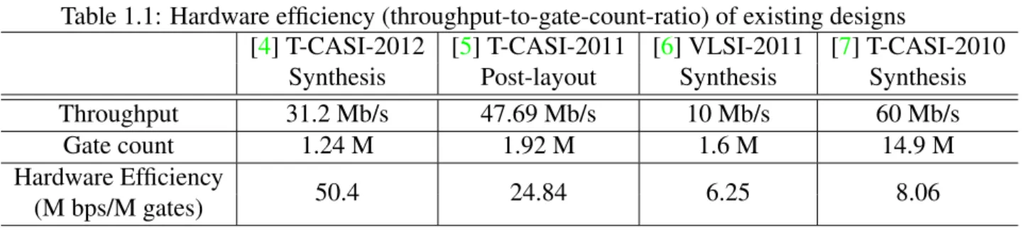
plement non-binary LDPC codes practically. In the state-of-the-art works, there are few designs can reach over 100 M bps in throughout and the gate counts all exceed 1 M as listed in Table 1.1. In order to enhance the hardware efficiency of non-binary LDPC codes decoder, we improve the throughput in CNU and VNU which are the main computation components in the decoder. In addition, we reduce the storage element of the edge messages and the channel values, and use layered scheduling to increase convergence speed.
Table 1.1: Hardware efficiency (throughput-to-gate-count-ratio) of existing designs
[4] T-CASI-2012 [5] T-CASI-2011 [6] VLSI-2011 [7] T-CASI-2010
Synthesis Post-layout Synthesis Synthesis
Throughput 31.2 Mb/s 47.69 Mb/s 10 Mb/s 60 Mb/s
Gate count 1.24 M 1.92 M 1.6 M 14.9 M
Hardware Efficiency
50.4 24.84 6.25 8.06
1.2
Thesis Organization
This thesis is organized as follows. In Chapter 2, we introduce the concept of non-binary low-density parity-check block codes and discuss several conventional decoding algorithms for non-binary LDPC codes. Chapter 3 will first introduce the conventional function units of non-binary LDPC decoder in hardware implementation. Then, the details of proposed function units and decoder architecture are provided. Chapter 4 gives the implementation results and the comparison with other related designs. Finally, conclusions and future works are given in Chapter 5.
Chapter 2
Principle of Non-binary Low Density
Parity Check Codes
Because of being the Shannon limit approaching codes, LDPC codes is an attractive solution in many communication and digital storage systems. Non-binary LDPC codes is an extension of binary LDPC codes, and it has excellent decoding ability and resist burst error. The more details about non-binary LDPC are prepared to discuss in section 2.2. In this chapter, we will first give the concept of the finite field. In addition, non-binary LDPC performance and its impact to system designs will be addressed. Finally, survey of available non-binary LDPC solutions will be briefly discussed.
2.1
Basic Introduction of Finite Field
A field contains only finitely many elements is called a Finite Field, or Galois Field. Like general field, finite field is also a framework for doing arithmetic, and it is closed under the operations defined like addition, subtraction, multiplication and division. Basic finite field can be constructed by a prime number p, and the field elements are 0, 1, ..., p− 1. In GF (p), a non-zero element a is called a primitive element if ap−1 = 1, and the powers of a generate the overall
as 0,1,α,...,αpm−1 based on the modulo p arithmetic, and the coefficient in polynomial form is 0, 1, ..., p− 1. The elements defined over GF(2p) are represented as binary sequence and have the advantage of easier arithmetic especially in addition. Therefore, binary finite field is widely used in several area like error control code (ECC) and cryptography.
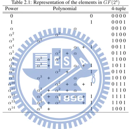
Table 2.1 shows an example of the three kinds of representation for GF (24) and the primitive polynomial is f (x) = x4+ x + 1.
Table 2.1: Representation of the elements in GF (24)
Power Polynomial 4-tuple
0 0 0 0 0 0 1 1 0 0 0 1 α α 0 0 1 0 α2 α2 0 1 0 0 α3 α3 1 0 0 0 α4 α + 1 0 0 1 1 α5 α2 + α 0 1 1 0 α6 α3 + α2 1 1 0 0 α7 α3 + α + 1 1 0 1 1 α8 α2 + 1 0 1 0 1 α9 α3 + α 1 0 1 0 α10 α2 + α + 1 0 1 1 1 α11 α3 + α2 + α 1 1 1 0 α12 α3 + α2 + α + 1 1 1 1 1 α13 α3 + α2 + 1 1 1 0 1 α14 α3 + 1 1 0 0 1
2.2
Non-binary LDPC Codes
In 1998 [1], Davey and MacKay extended the binary LDPC to the finite field GF (q), and the zero entries in H are replaced by the elements in finite field. It was shown that, non-binary LDPC codes can perform better than non-binary LDPC codes when the code length is small or applying to the higher-order modulation. Furthermore, non-binary LDPC can combat burst errors and further approach Shannon limit with good error floors. In [8], they confirm that non-binary LDPC codes outperform both convolutional turbo codes and quasi-cyclic LDPC codes for all code rate, modulation and codeword lengths. In addition, non-binary LDPC codes can
have good performance especially in more complex system, like MIMO and M-QAM channels [9]. In application, because of the good decoding ability and low throughput, non-binary LDPC codes are appealing solution for space/satellite communication systems [10] [11].
Even if non-binary LDPC codes have so excellent error correcting ability, but the rela-tively high complexity is always the main problem of the hardware implementation in practical. In order to figure out the efficient hardware implementation, several simplified versions from belief-propagation (BP) decoding algorithms are put forward in recent years. We will introduce some of them more detail in section 2.4.
2.3
Encoding of Non-binary LDPC Codes
The non-binary LDPC code is defined of the sparse parity check matrix H, and the con-struction of H are as follows. The matrix size of H is M rows by N columns, and (M ,N ) stand for the numbers of check equations (check nodes) and variable nodes respectively. In (2.1), the codeword c are defined as the null space of H, and the generator matrix G can be obtained by performing Gauss-Jordan elimination on H. The number of rows in G is represented as K, the length of information symbols. The entries of H are the elements which are defined in GF (q), and (dv,dc) stand for the column and row degree (or variable node and check node degree)
re-spectively. Note that the code is said regular if it has the same number of non-zero elements in all the columns and rows, otherwise it is called irregular code.
c = uG , GHT = 0 (2.1)
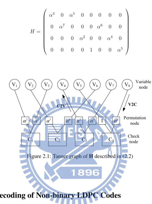
In (2.2) shows an example of (1,2) regular non-binary LDPC code over GF (8). Note that the code with dv=1 is not general, and it is for convenient to illustrate the example. The parity check
matrix H can be represented as a graphic form, called Tanner graph to illustrate the connection between variable nodes and check nodes. Based on the H described in (2.2), the correspond-ing Tanner graph is depicted in 2.1. In Tanner graph, the connections between variable and check nodes represent the non-zero elements in H, and the permutation node stands for the
corresponding symbol. H = α3 0 α5 0 0 0 0 0 0 α7 0 0 0 α6 0 0 0 0 0 α2 0 0 α4 0 0 0 0 0 1 0 0 α5 (2.2) V1 V2 V3 V4 V5 V6 V7 V8 C1 C2 C3 C4 3 α 5 α 7 α 6 α 2 α 4 α 11 5 α Variable node Check node Permutation node C2V V2C
Figure 2.1: Tanner graph of H described in (2.2)
2.4
Decoding of Non-binary LDPC Codes
Like binary LDPC, the decoding of non-binary LDPC codes is based on belief-propagation (BP) algorithm, or sum-product-algorithm (SPA) which iteratively updates the posterior prob-abilities of each variable node. In non-binary case, because the non-zero entries in H are not equal to 1, the arithmetic in finite field is required. In [12], the author proposed FFT-SPA to perform in the frequency domain, which transfers the complicated convolution operation into simpler multiplications. In order to further reduce the computational complexity, the decoding algorithm can be transferred to the logarithm domain [13]. In log-domain algorithm, it requires fewer quantization bits for storing message, and it is more robust to the quantization effect [14]. SPA (or BP) and FFT-SPA are the decoding algorithms without performance loss, but the
complicated computation and huge memory usage are very hard to be implemented in hard-ware. Therefore, the simplified versions with acceptable performance loss, like Extend Min-Sum (EMS) and Min-Max decoding algorithms are invented. In the following section, we will introduce SPA, EMS, and Min-Max decoding algorithms respectively. Except SPA, EMS and Min-Max are introduced in Log-Likelihood-Ratio (LLR) form. There are some comparison in complexity between several main decoding algorithms in non-binary LDPC codes, and it will be presented finally.
2.4.1
Sum of Product Algorithm (SPA)
In non-binary LDPC, the entries in H are defined in finite field, and the non-zero elements are not always equal to one. That is, the finite field multiplication is applied in check equations, and the single row check sum with degree dc over GF(2p) is shown in (2.3). Note that vi(x)
represents the variable symbol in polynomial form, and p(x) is the primitive polynomial.
dc
∑
i=1
hi(x)vi(x) = 0 mod p(x) (2.3)
In non-binary LDPC codes, the operation of multiplying the non-zero element in H is called permutation, and it is not required in binary LDPC decoding. Since the arithmetic operation in finite field is closed, the multiplication is a one-to-one mapping process. If the elements represented in power form, multiplication is actually a cyclic shift of whole elements in the field as shown in Figure 2.2. This is the reason that multiplication of the non-zero element in H in non-binary LDPC decoding procedure is called permutation.
Algorithm 1 shows the overall SPA decoding procedure in non-binary LDPC codes, and it is similar with the binary one except permutation and inverse permutation.
In Algorithm 1, one decoding iteration requires permutation, check node update, inverse permutation, and variable node update these steps to accomplish. In the following, we will discuss these processing steps in more details.
symbol 2
α
α
symbol 2α
α
α
×
Figure 2.2: Finite field multiplication over GF(22) with power form Algorithm 1:Decoding Procedure
Input: The messages after adding the channel noises Output: Decoded symbols
1 Initialization:
2 Initialize the channel value as the V2C message in the first time
3 while syndrome is zero or the maximum iteration number is reached do 4 Permutation:
5 Multiply C2V messages by corresponding non-zero element in H 6 Check Node Update:
7 Compute C2V messages based on the check equations 8 Inverse Permutation:
9 Multiply the corresponding non-zero inverse element in H 10 Variable Node Update:
11 Compute V2C messages and the posterior probability of each variable to decide
decoded symbols
12 Syndrome Computation: 13 Compute syndrome 14 end
the channel value and the message transmitted between nodes are all represented as a vector. The vector contains the possibility of each element defined in finite field, and the vector length depends on the size of the finite field. Note that in Figure 2.3, the two directions of message vector are represented as U (up) and D(down), and the direction from check node to variable node is U , and the other is D. The suffix of U and D stands for the incoming node and the outgoing node of this message vector. For example, DV C means the message vector going from
variable node to the check node. And DV C[i] stands for the possibility which the symbol of
the element is equal to i. Furthermore, LVj represents the channel value vector of variable node Vj, and LVj[i] stands for the possibility of channel value is equal to i. These notations are all
V1 V2 V3 V4 C1 C2 4 α 11 α5 Variable node Check node Permutation node 4 2 V C D 3 1 V C D 22 C V U 1 1 C V U 1 V L 2 V L 3 V L 4 V L 2 α
Figure 2.3: Notations used in non-binary LDPC decoding procedure
In the following, we will introduce these five decoding processes in the details.
1. Initialization
Using the information with the Gaussian additive noise from channel to calculate the probability of each element over GF(2p) in each variable node. Note that the symbol like-lihood value is denoted as L[i1, i2, ..., ip], and its polynomial form is
i(x) = (i1, i2, ..., ip) = p
∑
k=1
ikxk−1 (2.4)
For example, L[1, 0, 1] represents the possibility which the polynomial form of the ele-ment is x2+ 1 over GF(23).
Define bk is the kth bit of the symbol over GF(2p), and yk is the result after adding the
Gaussian noise nk. After transmitting in the channel, the corresponding possibility of
each symbol in variable node is calculated as
L[i1, i2, ..., ip] = p
∏
k=1
l(ik) (2.5)
In (2.5), l(ik) = probability(yk|bk = ik) and where yk = bk+ nk. Using the channel
value vector L as the V2C message vector in the first iteration.
In non-binary LDPC codes, the non-zero elements in the parity check matrix H are not only equal to 1, so the multiplication in the finite field is required when operating the check equations. Furthermore, the multiplication with inverse element after doing the check node update is also needed. In particular, the multiplication become much easier if the symbol of elements are stored as power form. Then, the multiplication is just to do the addition of the power items, and match the concept of naming permutation.
3. Check node update (CNU)
Using the incoming message DV C to update the check node of degree dc. According to
the combination of elements in the input vectors, to find out the check-sum set that satis-fies the check node equation such as
h1DV1C + h2DV2C+ h3DV3C = 0 (2.6)
and calculate the summation of all the elements in this check-sum set. Assume the updat-ing symbol in polynomial form is i(a)(x) of the m
thedge in Figure 2.4, and UCV[i
(a) 1 , i (a) 2 , ..., i (a) p ]
represents the possibility which the symbol in UCV vector is equal to a. The updating
equation is UCVm[i (a) 1 , i (a) 2 , ..., i (a) p ] = ∑ {..,i(a)(x),..| ∑dc l=1,l̸=mil(x)=i (a)(x)} dc ∏ k=1,k̸=m DVkC[i1, i2, ..., ip] (2.7)
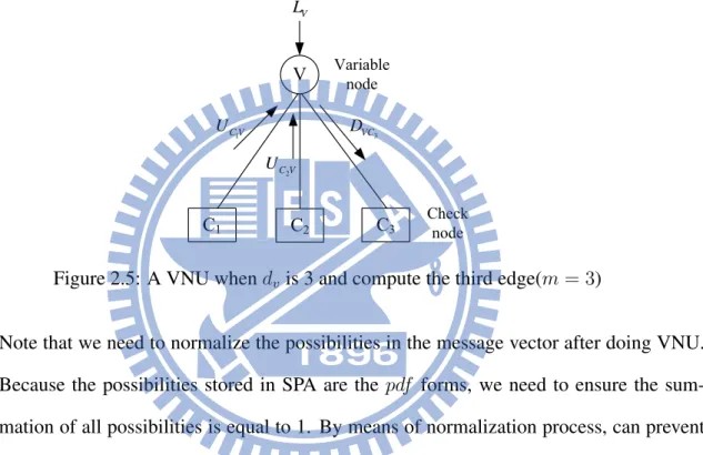
4. Variable node update (VNU)
In Figure 2.5, using the incoming message UCVs and the channel values to compute the
V2C messages (DV Cs) of degree dv. The (2.8) describes the computing function for the
case that updating symbol is a in the mthedge of variable node.
DV Cm[i (a) 1 , i (a) 2 , ..., i (a) p ] = LV[i (a) 1 , i (a) 2 , ..., i (a) p ] dv ∏ k=1,k̸=m UCkV[i (a) 1 , i (a) 2 , ..., i (a) p ] (2.8)
V1 V2 V3 C Variable node Check node 2 V C D 3 V C D 1 CV U V4 4 V C D
Figure 2.4: A CNU when dcis 4 and compute the first edge(m = 1)
V Variable node Check node 1 C V U 3 VC D C2 C3 C1 V L 2 C V U
Figure 2.5: A VNU when dv is 3 and compute the third edge(m = 3)
Note that we need to normalize the possibilities in the message vector after doing VNU. Because the possibilities stored in SPA are the pdf forms, we need to ensure the sum-mation of all possibilities is equal to 1. By means of normalization process, can prevent some possibilities to become very close to zero after several iteratively calculations.
5. Decision Unit
After an iteration every time, taking all the updated incoming messages of the variable node with the channel values to compute the posterior probabilities. Based on the q-ary probabilities, choose the largest one as the decoded symbol. According to the decoded symbols, the syndrome of each check equation is calculated. If the syndromes are not all zeros, the decoding process should be continued. But if there is no non-zero syndrome, the decoding process can be stopped even if the maximum iteration number is not reached called early termination.
2.4.2
Extended Min-Sum Algorithm (EMS)
The high computational complexity and the huge memory requirements are the main prob-lems for non-binary LDPC to implement in practical. In [15] [16], Extended Min-Sum (EMS) algorithm is to simplify the CNU computation, and truncate the message vector from the origi-nal field size q to a limited number denoted as nm. The nm elements are selected according to
the order of possibilities, so the message vectors need to store the first nm largest possibilities
and the corresponding symbols. Because of storing the incomplete messages, the compensated value γ is required to represent the possibility of the (q−nm) truncated elements. For simplicity, γ usually sets a constant value decided by performance simulation.
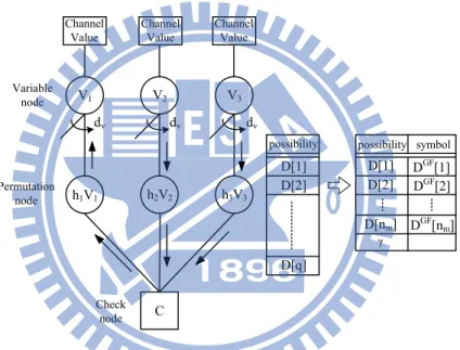
V1 V2 V3 h1V1 h2V2 h3V3 Channel Value Channel Value Channel Value dv dv dv Permutation node Variable node Check node possibility D[1] D[2] D[q] possibility symbol γ C D[1] D[2] D[nm] DGF[1] DGF[2] DGF[nm]
Figure 2.6: One check equation and edge message reduction in EMS decoding algorithm
Like SPA algorithm, we use U and D to represent the C2V and V2C message vectors re-spectively. Moreover, the notations for possibility and symbol of each element should be dis-tinguished. For example, U is still represented as the vector which stores the possibilities, but
U [i] changes to stand for the ith largest possibility (in SPA, U [i] stands for the possibility of
symbol i). And UGF[i] represents the corresponding symbol of U [i]. Note that the form of storing the possibilities can transfer to log-domain with Log-Likelihood-Ratio (LLR). It trans-form the complicated multiplication into simpler summations. In log-domain, the real-value addition transform to complicated operation related to logarithm, and EMS is to simplify it by
max function which is to find out the maximum among all inputs. Furthermore, it was shown
that arithmetic operation in log-domain are more robust to quantization effect, and the required number of quantization bits are also smaller. Assume P (a) is the possibility of symbol a, and the LLR form is calculated
U [k] = logP (U GF[k])
P (UGF[1]) k ∈ {1, 2, ..., nm} (2.9)
The decoding process of EMS algorithm is similar to the SPA decoding algorithm intro-duced in section 2.4.1. The most different thing is the simplified version of CNU, and the elements in edge message vector truncate to a limited size nm. In the following, the decoding
function based on the truncated messages with LLR form will be introduced.
1. Initialization
In general, the channel values are stored in complete field size in order to avoid perfor-mance loss. In the first iteration, sort out nmelements with the first nmlargest possibilities
be the V2C message vectors.
2. Variable Node Unit
Assume that the variable node degree is dv, and the updating function is
DV Cm[i (a) 1 , i (a) 2 , ..., i (a) p ] = LV[i (a) 1 , i (a) 2 , ..., i (a) p ] + dv ∑ k=1,k̸=m UCmV[i (a) 1 , i (a) 2 , ..., i (a) p ] (2.10)
In VNU, we need to combine the possibilities of identical symbols in (dv − 1) message
vectors. Because symbols in the message vector are stored by the order of possibility, the storing of symbols is non-regular and incomplete. Therefore, the operation of searching the same symbol from each input vector is required. If the identical symbol does not exist, it will be replaced by the compensated value γ.
3. Permutation and Inverse Permutation
In fact, the permutation and inverse permutation steps are just to do the multiplication in finite field, and the multiplicator is the non-zero element in parity check matrix H.
Because the set of symbols stored in message vector is incomplete, the set of symbols is changed after multiplying a symbol which is not equal to one. But for consistency, we still use ”permutation” to represent the multiplication with the non-zero elements in H.
4. Check Node Unit
In SPA, we need multiplications and summations to accomplish a CNU. Using the LLR form, the value multiplication can transform to simpler summation, but the real-value summation will become more complicated. For example, the addition like x1+ x2
changes to ln(ex1 + ex2). EMS is to simplify the summation related with logarithm to
max operation according to (2.11).
ln(ex1 + ex2) = max(x
1, x2) + ln(1 + e−|x1−x2|) (2.11)
Note that max operation is to find out the maximum from all inputs. Assume that the check node degree is dc, the updating function is.
UCVm[i (a) 1 , i (a) 2 , ..., i(a)p ] = max a= dc ∑ k=1,k̸=tak ( dc ∑ k=1,k̸=m DVmC[i (ak) 1 , i (ak) 2 , ..., i(ap k)]) (2.12)
Note that the output vector updated is still sorted in decreasing order. The function target of CNU is to sort out the first nmlargest possibilities from the candidate set. The example
of constructing a candidate set is illustrated in Figure 2.7 and Table 2.2. If the check node degree is dc, the size of the set is equal to n(dmc−1). Sorting from this huge set is too complex
to implement in practical. For this reason, in non-binary LDPC codes, we usually apply the approach like divide and conquer to simplify an updating function step by step [13].
In EMS algorithm, nmis a significant factor, and its size directly affects the performance on
hardware efficiency and decoding ability. It is a trade-off between hardware cost and decoding performance. Deciding the value of nmand figuring out a cost-performance balance is the most
V1 V2 V3 C 2 V C D 3 V C D 1 CV U V4 4 V C D γ 2 [4] V C D 2 [3] V C D 2 [2] V C D 2 [1] V C D 2 GF V C D 2(010) D 2 2(100) D 2(011) D 2(000) D γ 3 [4] V C D 3 [3] V C D 3 [2] V C D 3 [1] V C D 3 GF V C D 3(110) D 3 3(111) D 3(010) D 3(101) D γ 4 [4] V C D 4 [3] V C D 4 [2] V C D 4 [1] V C D 4 GF V C D 4(000) D 4 4(001) D 4(100) D 4(111) D
Figure 2.7: Update the first edge message UCV1 when dc = 4 and nm = 4
Table 2.2: Candidate set of the example in Figure 2.7
U1(000) U1(001) ... D2(010) + D3(110) + D4(100) D2(010) + D3(111) + D4(100) ... D2(010) + D3(010) + D4(000) D2(010) + D3(010) + D4(001) ... D2(010) + D3(101) + D4(111) D2(100) + D3(010) + D4(111) ... D2(100) + D3(101) + D4(001) D2(100) + D3(101) + D4(000) ... D2(011) + D3(111) + D4(100) D2(011) + D3(110) + D4(100) ... D2(011) + D3(010) + D4(001) D2(011) + D3(010) + D4(000) ... D2(000) + D3(111) + D4(111) D2(011) + D3(101) + D4(111) ... D2(000) + D3(110) + D4(111) ... D2(000) + D3(101) + D4(100) ...
performance loss in EMS is the least (< 0.1 dB) in all simplified non-binary LDPC decoding algorithms.
2.4.3
Min-Max Algorithm
In [17], Min-Max decoding algorithm is further simplifier than EMS decoding algorithm in check node processing. Based on the concept that the largest value dominates the result in addition, Min-Max replace the summation to max operation to reduce the computational complexity. The main differences in decoding process from EMS are initialization and CNU, so we describe these two steps in more detail as follows. Note that we use the complete field size without considering nmfor convenient in presenting the notations.
1. Initialization
Di(a) = ln(P (xi = si|channel)/P (xi = a|channel))
, where si is the most likely symbol f or xi
(2.13)
Note that P (x = a|channel) stands for the probability that the symbol representation of x is equal to a after adding the channel effect. The possibilities in message vector are initialized by (2.13), and the smaller value represents the higher possibility on the contrary.
2. Check Node Update (CNU)
Compared with the CNU computation in EMS, Min-Max replaces the summation to max operation in order to further simplify the updating function. Because of the overestima-tion in CNU, Min-Max is a little sub-optimal than EMS algorithm. The updating funcoverestima-tion in CNU is described by UCVm[i (a) 1 , i (a) 2 , ..., i (a) p ] = min a= ∑dc k=1,k̸=mak (max(DVmC[i (ak) 1 , i (ak) 2 , ..., i (ak) p ])) (2.14)
In (2.14), the min and max functions are to find out the minimum and maximum among all the inputs respectively. Because the smaller value stored in Min-Max decoding al-gorithm stands for the higher possibility, the CNU use min function to choose the most likely result.
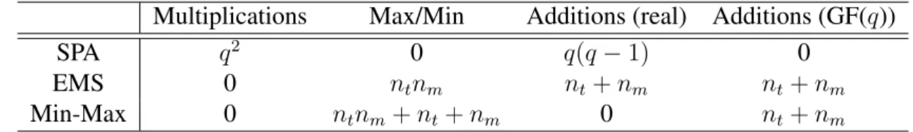
For the reason of simplicity, almost non-binary LDPC decoder are implemented by Min-Max algorithm, and there are many improved Min-Min-Max decoding algorithms are presented [7] [6] . In the following, the complexity in CNU and VNU with different decoding algorithms discussed in previous sections are presented [18] [19] [8], and the decoding performance is depicted in Figure 2.8. From the performance curve in Figure 2.8, the EMS is very close to FFT-SPA which is no performance loss, and outperforms than Min-Max about 0.2 dB. Supposing that it is defined over GF(q), and ntstands for the required clock cycles to accomplish a CNU
truncated number nm.
Table 2.3: Number of operations of check node updating function (dc = 2) for different
decod-ing algorithms
Multiplications Max/Min Additions (real) Additions (GF(q))
SPA q2 0 q(q− 1) 0
EMS 0 ntnm nt+ nm nt+ nm
Min-Max 0 ntnm+ nt+ nm 0 nt+ nm
Table 2.4: Number of operations of variable node updating function (dv = 2) for different
decoding algorithms
Multiplications Divisions Max Additions (real)
SPA q q 0 q− 1 EMS 0 0 nm(nm+ 2) nm Min-Max 0 0 nm(nm+ 2) nm 1 1.2 1.4 1.6 1.8 2 2.2 2.4 2.6 10−7 10−6 10−5 10−4 10−3 10−2 10−1 Eb/N0 (dB)
Bit Error Rate
FFT−BP EMS, n
m=32
Min−Max, n
m=32
Figure 2.8: Performance simulation for a (112,56) non-binary LDPC code over GF(26) with FFT-BP, EMS, and Min-Max decoding algorithms. The simulation is performed under BPSK modulation and AWGN channel. The maximum number of iterations is 50.
Chapter 3
Non-binary LDPC Decoder Architecture
In this chapter, we will first show the overall proposed decoder architecture. Then, the conventional approach for implementing each main function component in non-binary LDPC decoder with EMS algorithm [20] will be introduced. Following this, the proposed function units of the decoder are presented.
3.1
Non-binary Quasi-Cyclic LDPC Codes
Because of the code regularity and special code structure, QC-LDPC codes are an appeal-ing solution for VLSI implementation. Furthermore, QC-LDPC codes have good decodappeal-ing performance and relatively low error floor [21]. In our design, we also choose (2,4)-regular 64-ary non-binary QC-LDPC code to implement. Note that (2,4) stands for the column and row degrees respectively.
3.1.1
Code Structure
Quasi-cyclic code is composed of r by r sub-matrix with cyclic shift to identity matrix I0,
and the subscript of each I denotes the times of shift. With the feature of regularity in quasi-cyclic code, the complexity of decoder implementation can be simplified. Note that the block row stands for the r rows grouped by sub-matrices, and the same as block columns.
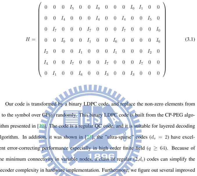
The non-binary QC-LDPC code used in our design is described in (3.1) H = 0 0 0 I5 0 0 I0 0 0 0 I0 I1 0 0 0 0 I4 0 0 0 I4 0 0 I4 0 0 I5 0 0 I7 0 0 0 I7 0 0 0 I7 0 0 0 I0 0 0 I0 0 0 I1 0 0 I6 0 0 0 0 I6 I2 0 0 0 I1 0 0 0 I1 0 0 0 I2 0 I4 0 0 I7 0 0 0 I7 0 0 0 I7 0 0 0 I1 0 0 I6 0 0 I3 0 0 I3 0 0 0 (3.1)
Our code is transformed by a binary LDPC code, and replace the non-zero elements from 1 to the symbol over GF(q) randomly. This binary LDPC code is built from the CP-PEG algo-rithm presented in [22]. The code is a regular QC code, and it is suitable for layered decoding algorithm. In addition, it was shown in [23], the ”ultra-sparse” codes (dv = 2) have
excel-lent error-correcting performance especially in high order finite field (q ≥ 64). Because of the minimum connectivity in variable nodes, a class of regular (2,dc) codes can simplify the
decoder complexity in hardware implementation. Furthermore, we figure out several improved approaches in edge memory reduction and efficient VNU processing based on this property. And this code can be separated into two sub-blocks from the middle in matrix, because these two sub-blocks contain the same number of non-zero sub-matrices in each block row. For this reason, if we want to increase the memory banks for improving bandwidth, it is a convenient property for configuring the memories.
3.2
Decoder Architecture
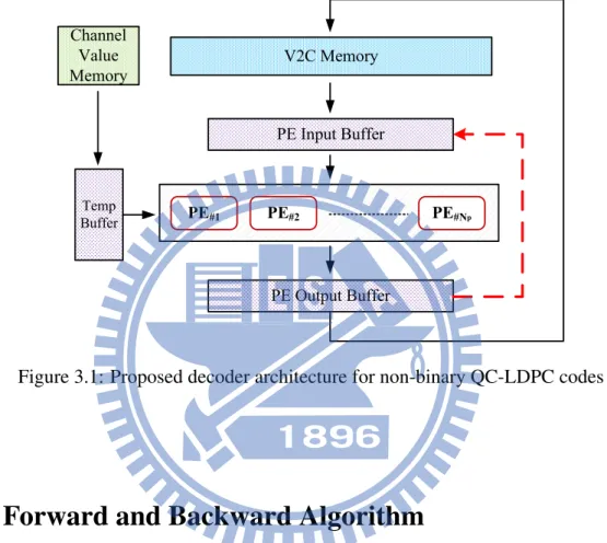
Figure 3.1 shows the overall decoder architecture, and it is mainly composed of several Processing Elements (PEs), storage elements , and control circuits. A PE is composed of one
CNU and its associated VNUs, and it is the main computation unit in our proposed design. Furthermore, Np stands for the number of parallelism when implementing the decoder, and the
number of Np is directly affect the throughput and hardware cost. Note that the dashed line is
the extra bypass path to solve the memory collision problem which will be discussed in 3.6.3.1.
PE#1 PE#2 PE#Np
V2C Memory PE Input Buffer PE Output Buffer Temp Buffer Channel Value Memory
Figure 3.1: Proposed decoder architecture for non-binary QC-LDPC codes
3.3
Forward and Backward Algorithm
In non-binary LDPC codes, the complexity of updating function grows in exponential ac-cording to the number of node degrees. For this reason, using the efficient approach called forward and backward algorithm [24], which is a recursive structure like the concept of divide and conquer to accomplish the updating function step by step. First, the updating function is decomposed by several basic functions called elementary steps, and then executing the elemen-tary steps recursively to accomplish an updating function. An elemenelemen-tary step is defined as an updating function composed of only 2 input vectors and 1 output vector. In general, if the node degree is equal to d, it requires 3(d− 2) elementary steps to finish a node updating function. Figure 3.2 illustrates the required elementary steps and the corresponding forward/backward
recursive structure when the check node degree dcis equal to 4. (a) (b) V1 V2 V3 V4 CNU CES CES CES in the first stage CES in the second stage CES V1 V2 V3 V4 CES I3,4 I1,2 4 CV U 3 CV U 2 CV U 1 CV U CES CES CES CES 1 CV U 2 CV U 3 CV U 4 CV U
Figure 3.2: (a) A CNU with dc= 4 (b) Forward/Backward recursive structure with dc= 4
The following describe a check node (dc= 4) updating procedure with the forward/backward
algorithm. At the first stage, using 2 Check Elementary Steps (CES) to compute 2 inter-nal vectors, I1,2 and I3,4. Note that I1,2 stands for the internal message vector containing
the information from input vectors V1 and V2. At the second stage, the 4 output vectors
(UCV1,UCV2,UCV3,UCV4) are computed from the combination of each input vector and the 2
internal results calculated in the first stage. Therefore, in the case that dcis equal to 4, we need
3(4− 2) = 6 elementary steps and 2 stages to accomplish a check node updating function.
3.4
Check Node Unit (CNU)
Check node unit (CNU) is the most complicated component in non-binary LDPC decoding procedure, and it is usually the bottleneck when implementing the decoder in practical. Based on the forward and backward recursive structure, a CNU is decomposed of several check ele-mentary steps (CESs) to implement. In this section, we first introduce the conventional approach in processing a CES, and then an efficient algorithm [25] especially target on simplifying the CES in EMS decoding algorithm is addressed. Following this, we will present our proposed CES architecture for improving the throughput without extra decoding performance loss.
3.4.1
Check Elementary Step (CES)
Check elementary step (CES) is an updating function of degree 2, and it is assumed that the input vectors already finish the permutation step. Suppose the vector size is nm, and the
notations of input and output vectors are I1, I2, and O respectively. Note that the possibilities
in each message vector are represented as log-likelihood-ratio (LLR) and sorted in decreasing order. Define a candidate set Sc, and the elements in Sc are the combinations from the input
vectors which satisfy the equation I1GF[i]⊕ IGF
2 [j] = OGF[k] and the corresponding possibility
is I1[i] + I2[j] = O[k]. Then, the goal of CES is to explore the non-repeating symbols with the
first nmlargest possibilities from Sc. The equation of CES to compute the kthlargest possibility
is
O[k] = max
I1GF[i]⊕I2GF[j]=OGF[k] i,j∈[1,nm]2
{I1[i] + I2[j]} (3.2)
There are n2
m elements in candidate set Sc, and exploring in whole Scis very complicated.
Using the sorted property in each message vector, the more efficient way to realize a CES is to search elements from the graphic form [24]. Define a candidate map called M as shown in Figure 3.3, and M displays the possibilities distribution of the n2
m elements in Sc. In order to
reduce the size of Sc, the author in [24] proposed a ”sorter” which stores nm candidates for
exploring at a time, and then the size of Scchanges from n2m to nm. Note that candidate set Sc
is redefined as the elements in the sorter, and it updates every cycle.
Based on the candidate map M and a sorter of size nm, the processing operations of CES
using graphic approach are as follows [20]. Note that the meaning of sorting used in EMS algorithm is to insert one element into a sorted sequence denoted as sorter.
1. Initialization
Insert nm elements in the first column of M into the sorter.
2. Output
Output an element with the largest possibility in the sorter.
S P 1 16 4 2 8 13.2 11.7 10.1 7.9 6 24 20.3 25 8 28 26 16 33.5 32 30.4 28.2 26.3 8 17.1 9 24 12 10 0 30.3 28.8 27.2 25 23.1 3 15 2 19 7 1 11 28.2 26.7 25.1 22.9 21 15 13.4 14 31 11 13 7 26.6 25.1 23.5 21.3 19.4 7 11.1 6 23 3 5 15 24.3 22.8 21.2 19 17.1
Figure 3.3: Candidate map M , (S,P) stands for symbol and possibility respectively
Check whether the symbol is redundant. If this symbol is already in the output vector, discard this symbol. This operation is implemented by p bits comparator circuit when the symbol is defined over GF (2p).
4. Candidate Choose
Choose the right side symbol of the output symbol as the candidate inserting to the sorter.
5. Sort
According to the possibility, insert the candidate symbol into the sorted sequence in the sorter.
Repeat step 2 to step 5 till output vector is full or the predetermined processing cycles is reached. The operations are described in Algorithm 2, and Figure 3.4 illustrates a CES procedure.
If message vector contains the repeated symbols, it means that the valid number of nm
becomes smaller. After iteratively decoding process, the valid symbols will be fewer and fewer and result in the significant decoding performance loss. Therefore, the operation of symbol checking is necessary, and the repeated symbols should be discarded.
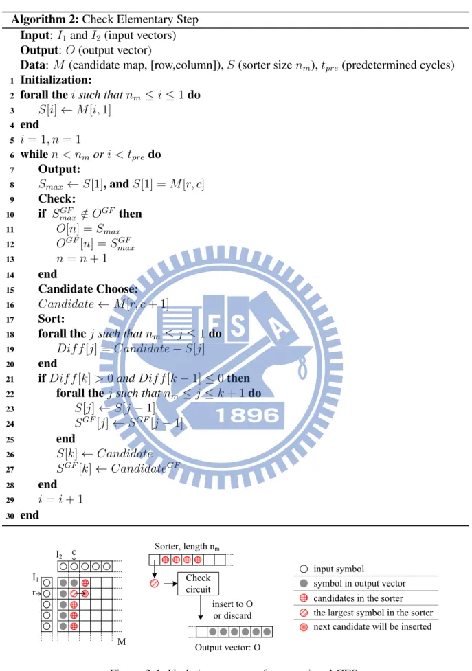
Algorithm 2:Check Elementary Step Input: I1 and I2(input vectors)
Output: O (output vector)
Data: M (candidate map, [row,column]), S (sorter size nm), tpre(predetermined cycles)
1 Initialization:
2 forall the i such that nm ≤ i ≤ 1 do
3 S[i]← M[i, 1] 4 end 5 i = 1, n = 1 6 while n < nmor i < tpredo 7 Output: 8 Smax ← S[1], and S[1] = M[r, c] 9 Check: 10 if SmaxGF ∈ O/ GF then 11 O[n] = Smax 12 OGF[n] = SmaxGF 13 n = n + 1 14 end 15 Candidate Choose: 16 Candidate ← M[r, c + 1] 17 Sort:
18 forall the j such that nm ≤ j ≤ 1 do
19 Dif f [j] = Candidate− S[j]
20 end
21 if Dif f [k] > 0 and Dif f [k− 1] ≤ 0 then 22 forall the j such that nm ≤ j ≤ k + 1 do
23 S[j]← S[j − 1] 24 SGF[j]← SGF[j − 1] 25 end 26 S[k]← Candidate 27 SGF[k]← CandidateGF 28 end 29 i = i + 1 30 end Sorter, length nm Output vector: O I1 I2 input symbol
symbol in output vector candidates in the sorter the largest symbol in the sorter next candidate will be inserted M c r Check circuit insert to O or discard
3.4.2
Bubble Check Algorithm
In [24], the author proposed a method to reduce the number of elements when searching the largest possibility, and the size of candidate set Sc is smaller than nm. Every clock cycle, the
operation of a CES is to find out an element with the largest possibility from the sorter. For this reason, it just needs to ensure that the element with the largest possibility is in the sorter in every clock cycle. Bubble check algorithm [25] uses this property to efficiently reduce the number of elements in Sc at one time. It means that only the element which probably has the
largest possibility at that time will be considered, and this is based on the regular distributing property of possibilities in M .
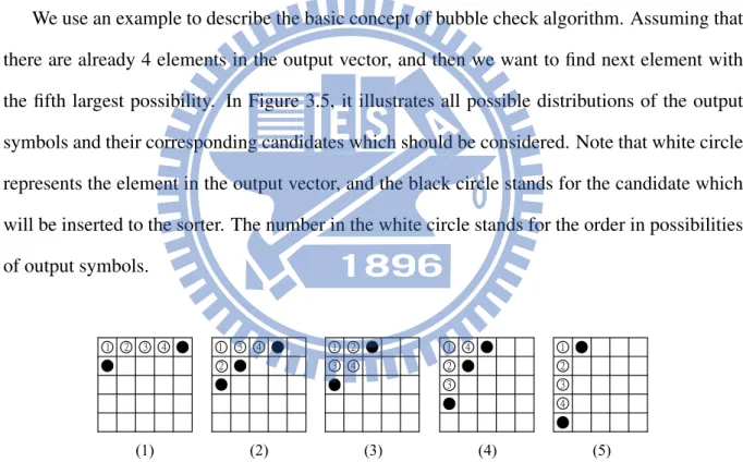
We use an example to describe the basic concept of bubble check algorithm. Assuming that there are already 4 elements in the output vector, and then we want to find next element with the fifth largest possibility. In Figure 3.5, it illustrates all possible distributions of the output symbols and their corresponding candidates which should be considered. Note that white circle represents the element in the output vector, and the black circle stands for the candidate which will be inserted to the sorter. The number in the white circle stands for the order in possibilities of output symbols. (1) (2) (3) (4) (5) 1 2 3 4 1 3 4 2 1 2 4 3 1 2 3 4 1 2 3 4
Figure 3.5: 5 possible conditions when finding the 5thlargest possibility.
According to the possibilities stored in input vectors are in decreasing order, the larger possibilities are centralized in the upper left of M . Based on the regularity in M , candidates choosing are decided from the right or down side of the output symbols. Because bubble check algorithm only considers the possible candidates with the largest possibility, we do not need to take account of more than one elements in the same row or the same column. Therefore,
the minimum required number of candidates depends on the distributing shape of the output symbols. In the second and forth graphs, when the distributing shape is close to triangular, the number of possible candidates is more. Looking into other graphs, the number of candidates is the least when the distributing shape of the output symbols is rectangular. After considering these five situations, we can infer that the minimum required sorter size with nm5 should be 3.
Therefore, the minimum required sorter size depends on the distributing shape of elements in the output vector, and the worst case is when the distributing shape is triangular. Without considering the symbol repetition problem, the sorter size ns is calculated by supposing there
are already (nm− 1) symbols in the output vector and the distributing shape of these symbols
is triangular. The relation between nm and ns is described by
(1+ns)ns 2 = (nm− 1) + ns ⇒ ns = ⌈ 1+√1+8(nm−1) 2 ⌉ (3.3)
Table 3.1: The relation between nsand nm
nm 4 8 16 32 64
ns 3 5 6 9 12
Based on (3.3), the number of nswith different nmare listed in Table 3.1. The process of the
CES applying the bubble check algorithm is similar with conventional CES mentioned above, and the main difference is the smaller sorter size nsand the way of choosing the candidate. The
procedures are illustrated in Figure 3.6 and the operations are described as follows:
1. Initialization
Insert nssymbols in the first column of M to the sorter.
2. Output
Output the symbol with the largest possibility in the sorter.
3. Check
Check whether the symbol is redundant. If this symbol is already in the output vector, discard this symbol.
I2 1 I1 M Sorter (size=nm=4) 4 8 9 2 5 3 7 6 10 11 12 13 14 15 16 1 2 3 6 1 4 8 9 2 5 3 7 6 10 11 12 13 14 15 16 1 2 3 6 1 2 3 6 Output vector Check Discard 1 1 4 8 9 2 5 3 7 6 10 11 12 13 14 15 16 2 3 6 1 4 8 9 2 5 3 7 6 10 11 12 13 14 15 16 2 3 6 4 Sort 1 4 8 9 2 5 3 7 6 10 11 12 13 14 15 16 2 3 4 6
Figure 3.6: Procedure of bubble check algorithm in the beginning.
4. Candidate choose
(a) If the output symbol is in the first column/row, choose its down/right side symbol as the candidate. (b) If not, maintain the same direction with last clock cycle.
5. Sort
According to the possibility, insert the candidate symbol into the sorted sequence which is reduced to ns.
Repeat (2) to (5) till output vector is full or the predetermined processing cycles is reached. The overall processing steps are described in Algorithm 3.
In bubble check algorithm, it needs to decide the candidate from right or down side of the element with the largest possibility as shown in Figure 3.7(a). This increases some complexity in the controlling circuit when choosing candidate. In order to simplify the controlling circuit, L-bubble check [26] is to determine the paths of choosing next candidate in advance. There is an example when ns is equal to 4 in Figure 3.7(b), and the elements in dark zone will not be
considered.
Algorithm 3:Check Elementary Step with Bubble Check Algorithm Input: I1 and I2(input vectors)
Output: O (output vector)
Data: M (candidate map), S (sorter size ns), flag (the direction of candidate choosing)
1 Initialization:
2 forall the i such that ns≤ i ≤ 1 do
3 S[i]← M[i, 1] 4 end 5 i = 1, n = 1 6 while n < nm do 7 Output: 8 Smax ← S[1], and S[1] = M[r, c] 9 Check: 10 if SmaxGF ∈ O/ GF then 11 O[n] = Smax 12 OGF[n] = SmaxGF 13 n = n + 1 14 end 15 Candidate Choose: 16 if r = 1 then 17 f lag← 0 18 else if c = 1 then 19 f lag← 1
20 else if M [r + f lag, c +f lag]¯ ∈ S then
21 f lag← ¯f lag
22 else
23 f lag← flag
24 end
25 Candidate ← M[r + flag, c + ¯f lag]
26 Sort:
27 forall the j such that ns ≤ j ≤ 1 do
28 Dif f [j] = Candidate− S[j]
29 end
30 if Dif f [k] > 0 and Dif f [k− 1] ≤ 0 then 31 forall the j such that nm ≤ j ≤ k + 1 do
32 S[j]← S[j − 1] 33 SGF[j]← SGF[j − 1] 34 end 35 S[k]← Candidate 36 SGF[k]← CandidateGF 37 end 38 i = i + 1 39 end
number of candidates and have√nm complexity reduction [25]. But like traditional CES, it
(a) (b)
Figure 3.7: (a) The illustration of choosing the candidate from right or down direction (b)Example of predetermined path for ns = 4 in L-bubble check algorithm
output vector. In average, the processing time of a CES is equal to 2nm cycles for avoiding the
performance loss as shown in Figure 3.8. For this reason, if we want to improve the throughput, the processing cycles in a CES should be reduced.
1.4 1.6 1.8 2 2.2 2.4 2.6 2.8 10−7 10−6 10−5 10−4 10−3 10−2 10−1 (112,56), R=1/2,Iteration=50,BPSK E b/N0 (dB)
Bit Error Rate
2n
m processing cycles
n
m processing cycles
no predetermined cycles
Figure 3.8: Performance curve when the processing cycles is decided as nm and 2nm. No
predetermined cycles stands for the case that the CES stop computing until output vector is full.
3.4.3
Proposed Check Elementary Step
As mentioned in last section, 2nm clock cycles are required in processing the CES because
of the repeated symbols. There is still no efficient way to filter out the redundant symbols in candidate choosing step, so 2 times nm processing cycles in CES is unavoidable. For this
reason, the proposed method of improving the throughput in CES is directly to double the output symbol at a time.
3.4.3.1 Proposed Double Throughput Bubble Check Algorithm
According to the target of double throughput, we modify the approach in candidate choosing step and output 2 symbols at a time. Supposing that (nm,ns) is (7,5), we introduce the candidates
choosing procedure with Figure 3.9, and discuss in the followings.
(a) (b) (c) (d) (e)
(f) (g) (h)
Symbol in output vector Symbol in sorter Output symbol Temporary candidate
Figure 3.9: Candidate choosing procedure of double throughput bubble check, (nm,ns) = (7,5)
In original bubble check algorithm, it guarantees that the sorter contains the element with the largest possibility. But in our proposed method, the sorter output 2 elements at a time, so the first 2 largest possibilities should be considered. For this reason, the distribution for initialization is a little different from conventional one, and it is depicted in (a). The next 2 candidates are chosen among 4 temporary candidates, so we need to decide 4 temporary candidates first. These 4 temporary candidates are the right and down side symbols of the 2 output symbols. It is needed to check that these 4 temporary candidates should be the element with the largest possibility in its row or column as illustrated in (f) and (h). From this example, it is too complicated in controlling the direction of deciding the next 2 candidates. Therefore, we combine the L-bubble check algorithm to simplify the controlling circuit.
3.4.3.2 Proposed Double Throughput L-bubble Check Algorithm
In general, the paths for choosing candidates are determined after performance simulation, and we first define 2 regions in M for describing the procedure easily. In Figure 3.10, the darked zone in the first row and first column is denoted as region a, and the rest predetermined paths is region b. In our proposed method, if the output symbol is in region a, we need extra computation to decide the candidate.
x y
m
n
Region a Region b
Elements in output vector Elements in sorter
Figure 3.10: Candidate map M used in proposed CES
We use an example illustrated in Figure 3.11 to describe the procedure which the output symbol is in the region a. Every time, using 4 possibilities (x, y, m, n) and 3 comparators to determine the first 2 largest possibilities in region a, and we denote 1 and 2 in the circles to represent them. Then, depends on the number of output symbols in the region a to decide the next candidate. And Figure 3.12 shows the performance loss when directly applying the L-bubble check algorithm without separating the regions.
x y m n 1 2 x y (a) (b)
Elements in output vector Elements in sorter Output symbol Candidate in region a
m n
Algorithm 4: Candidates Choose in CES with Proposed Double Throughout L-Bubble Check Algorithm
Input: S1 and S2(output elements with the first 2 largest possibilities), M [r1, c1] and
M [r2, c2] (the corresponding position in M )
Output: C1and C2 (the candidates prepared to insert to the sorter)
Data: Region a: path1 records the position for current symbol in the sorter of the first
row, pathns records the position for current symbol in the sorter of the first
column. Region b: (Lr,Lc) represents the predetermined path
1 Extra 2 Candidates in Region a, Ca1and Ca2(x, y, m, n are defined as Figure 3.11): 2 p1 = x− m, p2 = x− n, p3 = m− y
3 if [sign(p1), sign(p2), sign(p3)] = [0, 0, 1] then
4 Ca1 ← M[1, c(path1) + 1], Ca2 ← M[1, c(path1) + 2] 5 else if [sign(p1), sign(p2), sign(p3)] = [0, 0, 0] then
6 Ca1 ← M[1, c(path1) + 1], Ca2 ← M[r(pathns) + 1, 1]
7 else if [sign(p1), sign(p2), sign(p3)] = [1, 1, 0] then
8 Ca1 ← M[r(pathns) + 1, 1], Ca2 ← M[r(pathns) + 2, 1] 9 else
10 Ca1 ← M[r(pathns) + 1, 1], Ca2 ← M[1, c(path1) + 1] 11 end
12 Decide C1and C2 :
13 if Both M [r1, c1] and M [r2, c2] are in regin a then 14 C1 ← Ca1, C2 ← Ca2
15 else if M [r1, c1] is in regin a, M [r2, c2] is in regin b then 16 Cb1 ← M[r2+ Lr, c2+ Lc]
17 C1 ← max(Ca1, Cb1), C2 ← min(Ca1, Cb1)
18 else if M [r1, c1] is in regin b, M [r2, c2] is in regin a then 19 Cb1 ← M[r1+ Lr, c1+ Lc] 20 C1 ← max(Ca1, Cb1), C2 ← min(Ca1, Cb1) 21 else 22 Cb1 ← M[r1+ Lr, c1+ Lc], Cb2 ← M[r2+ Lr, c2+ Lc] 23 C1 ← max(Cb1, Cb2), C2 ← min(Cb1, Cb2) 24 end
The overall operations are as follows:
1. Initialization
Insert (ns − 1) symbols in the first column and second symbol in the first row into the
sorter. Because we want to ensure that there are at least two symbols in the first column and the first row. In Figure 3.10, the white circles represent the initialization when ns is
equal to 4.
2. Output
1 1.2 1.4 1.6 1.8 2 2.2 2.4 2.6 10−6 10−5 10−4 10−3 10−2 10−1 100 (112,56), R=1/2,Iteration=50,n m=32,BPSK E b/N0 (dB)
Bit Error Rate
w/ regions
w/o regions
Figure 3.12: Performance comparison of defining regions
3. Check
Check whether these two symbols are already in the output vector. If yes, give up the redundant symbols.
4. Candidate choosing
(a) If output symbol is in region a, choose the candidates from the 2 candidates, Ca1 and
Ca2. (b) If output symbol is in region b, choosing the candidate followed predetermined
path.
5. Sorting
Insert two candidates C1and C2 into the sorter, and C1is larger than C2.
Using our proposed double throughput L-bubble check algorithm, there is no decoding per-formance loss compared with conventional one, and the processing time in a CES reduces to
nm cycles. The decoding performances of several decoding algorithms and our proposed one
1 1.2 1.4 1.6 1.8 2 2.2 2.4 2.6 10−7 10−6 10−5 10−4 10−3 10−2 10−1
(112,56), R=1/2,Iteration=50,BPSK
E
b/N
0(dB)
Bit Error Rate
FFT−BP EMS, n m=32 Min−Max, n m=32 Proposed, n m=32
Figure 3.13: Comparison with other conventional algorithms
3.5
Variable Node Unit (VNU)
Target on the (2,dc) non-binary LDPC codes, we proposed an efficient architecture to
imple-ment the variable node unit (VNU) with less memory usage. In the following sections, we first introduce the conventional variable elementary step (VES), and then the proposed VNU will be presented. The final parts in this section are the decision unit and proposed function unit which contains CES, VNU, and decision unit.
3.5.1
Variable Elementary Step (VES)
A VES is composed of two input vectors and one output vector, and the updating function is the following. O[k] = max IGF 1 [i]=I2GF[j]=OGF[k] i,j∈[1,nm] {I1[i] + I2[j]} (3.4)
The goal of a VES is to sort out the first nm largest message possibilities among the 2nm
elements involved in the two input vectors. Assume that I1 and I2 are the input vectors and O
is the output vector of the VES, and each vector size is equal to nm. The updating process is
1. Candidates computation
First nm cycles: According to the elements in I1, search for the element with identical
symbol from I2 and combine their possibilities. If there is no corresponding identical
symbol, adding the compensation value of I2 to replace it.
Second nm cycles: Add the possibility of each symbol in I2 with the compensation value
of I1. C[i] = I1[i] + I2[j] if I1GF[i] = I2GF[j] γI2 if I GF 1 [i] /∈ I2GF , CGF[i] = I1GF[i] C[i + nm] = γI1 + I2[i] , C GF[i + n m] = I2GF[i] i∈ [1, 2, ..., nm] (3.5)
The function of candidates computation is described in (3.5). Note that C represents as a vector which size is 2nm for storing the candidates, and γ1 and γ2 stand for the
compensation value of I1and I2 respectively.
2. Insert
According to the possibility calculated, insert the candidate into the output vector in de-creasing order. If the identical symbol already exists in O, discard this candidate element. Repeat these two steps for 2nmclock cycles, and the VES updating procedure is described
in Algorithm 5.
In VES, it needs nm ”symbol matching” circuits to search identical symbol from nm
ele-ments in I2as shown in Figure 3.14, and a symbol matching circuit is to check whether 2 inputs
are the same or not. The conventional VES needs 2nm cycles to process, and maybe several
repeated symbols are accessed in these cycles. Therefore, we try to figure out the more efficient way to implement the VES without consuming redundant cycles on the repeated symbols.