近場通訊系統之天線耦合分析

國立臺灣大學電機資訊學院電信工程學研究所 碩士論文

Graduate Institute of Communication Engineering College of Electrical Engineering ＆ Computer Science

National Taiwan University Master Thesis

近場通訊系統之天線耦合分析

Analysis of Antenna Coupling in Near-Field Communication Systems

陳晏笙 Yen-Sheng Chen

指導教授：李學智 博士 Advisor: Hsueh-Jyh Li, Ph.D.

中華民國 98 年 6 月

June, 2009

國立臺灣大學碩士學位論文 口試委員會審定書

近場通訊系統之天線耦合分析

Analysis of Antenna Coupling in Near-Field Communication Systems

本論文係陳晏笙君（R96942002）在國立臺灣大學電信工程學研 究所完成之碩士學位論文，於民國 98 年 06 月 13 日承下列考試委員 審查通過及口試及格，特此證明

口試委員：

系主任、所長

致謝

很榮幸能在台大電信所碩士班就讀兩年。首先要感謝指導教授李學智教授。

老師身教謙虛而正義的品格，鼓勵我們要將台大的栽培回饋社會；提供我們最多 的研究資源，使實驗室有自由而積極的學風。感謝陳士元教授，這一年來多次和 老師隔海語音討論，從中學習到研究的方法、思考邏輯，以及做學問的態度；老 師總是不厭其煩的指導我許多細節，並且幫助我修改投稿的期刊論文。因為兩位 老師的指導，使我在研究所的成長遠超出大學畢業時的自我期許，也讓我有信心 迎接下個階段博士班的挑戰。其次，我也要感謝口試委員陳俊雄教授、江衍偉教 授、楊成發教授、唐震寰教授給我的建議，使我的論文更完備。

我很喜歡這一年來實驗室的研究風氣，認識了許多好朋友。感謝博士班學姊 文方，學長柏仁、均哲、偉傑、家杰、念恩、易洵、貴程、蒲平日之照顧。謝謝 宗穎，除了在研究上幫助我，平時我們一起聊天、打球、玩樂，都會是我珍貴的 回憶。感謝建伯幫我修改論文的英文，以及平日的討論與協助。也謝謝同學得勝，

曾經陪我在無反射室量測到半夜才回家。謝謝學弟李明，和你聊運動比賽總是很 有趣；而且玩 MVP 當我被拉開，你都會投幾個內角高讓我打。學弟昱超，你是我 看過最乖的小孩，做事總是能讓人放心。還有貼心的力涵，畢業典禮從你們手中 接過拼圖卡片的那一刻，我真的很感動。因為有你們這些好朋友，讓我來實驗室 都覺得很開心。感謝好友奕嘉，雖然我們高中是同班同學，但真正了解你卻是在 研究所的階段；每次有事麻煩你，你總是義無反顧的幫忙。我會珍惜這份友誼，

也祝你服研發替代役的日子順利。謝謝在我碩士生涯尾聲出現的小天使—忻恩，

因為妳的出現，才讓我在博士班一切順利無懼任何挑戰；有妳的照顧與陪伴，我 才能在人生的道路全心全力勇往直前。

最後，要感謝我生命中最重要的家人。感謝父母對我的栽培，讓我的求學過 程一路順遂。我努力的想讓您們以我為榮，報答您們的養育之恩。能做您們的孩 子，是我這輩子最大的福氣。也要謝謝小舅舅蔡銘昌博士，在我求學的過程中總 是支持我，給我許多指點與建議。然後，我想要告訴奶奶，來不及讓您看到我碩 士畢業，但您永遠活在我心裡。

這篇論文的完成是我生命中重要的一頁，僅將此篇論文獻給曾經幫助過我的 人們。

摘要

近年來，近場通訊系統的應用日趨廣泛，諸如超高頻近場射頻辨識系統、近 距離無線通訊技術(NFC)。在近場通訊系統中，我們希望成功的設計天線，並優化 系統的效能，因此收發兩端的天線耦合分析就變得很重要。本論文提出一個簡單 的公式，可以計算近場通訊系統中傳送天線和接收天線之間的功率耦合係數(power coupling coefficient)。此公式的適用性不拘天線的種類、形式、尺寸、工作頻率；

所需的資訊為收發兩端天線在該工作頻率下的三維遠場場形、天線之間的相對傾 斜角度及距離。換言之，我們所提出的公式可視為遠場福利斯傳輸方程式(Friis transmission equation)在近場的類比。

為了驗證公式的準確性，我們先考慮幾種常用的天線，利用他們的場形標準 式(close-form pattern)，將計算的近場耦合係數和全波分析模擬(HFSS)作比較。此 外，我們也以超高頻近場射頻辨識系統為例，設計符合此應用的天線，並且比較 量測、模擬、理論計算的結果。透過這些驗證，我們確認所提出的公式可以精準 的算出近場功率耦合係數。在實驗中我們也發現了一些影響耦合程度的參數，諸 如接收天線的阻抗匹配、發送天線的指向性。藉由提出的公式，我們還可以計算 超高頻近場射頻辨識系統的讀取距離以及可靠度。因此，這篇論文提出的成果相 信有助於應用在近場通訊系統。

關鍵詞 — 電磁耦合、近場、能量傳輸、射頻辨識、超高頻天線。

Abstract

Recently, near-field communication systems have been widely used in many applications such as the near-field UHF RFID item-level tagging, the Near Field Communication (NFC) device, and the mCoupons. To successfully design and optimize the near-field communication systems, it is important to investigate the near-field coupling between the transmitting and receiving antennas. In this thesis, a simple formula has been presented for computing the coupling coefficient between two antennas that are placed in the near field of each other. The choices of the two antennas are arbitrary, and all the information needed includes the corresponding normalized vector far-field patterns along with their relative orientations and the antenna spacing.

To verify the proposed formulation, the coupling coefficients in several near-field scenarios, including a practical near-field UHF RFID system, are computed and compared to those measured and full-wave simulated using Ansoft HFSS. They are all in good agreement. Additionally, it is shown that several factors may influence the coupling coefficient, such as the impedance matching of the receiving antenna and the directivity of the transmitting antenna. With the aid of the proposed formulation, the near-field read range and read reliability can be determined and the near-field coupling phenomena can be investigated. The results thus obtained may be useful in the near-field communication systems.

Keywords — Electromagnetic coupling, near field, power transmission, RFID, UHF antennas.

Contents

Abstract I Contents III List of Figures V List of Tables VII

Chapter 1 Introduction 1

1.1 Motivation...1

1.2 Thesis Overview...3

Chapter 2 Near-Field Coefficient 5

2.1 Introduction………...5

2.2 Antenna Field Region………...6

2.3 Antenna Coupling versus Longitudinal Displacement...7

2.3.1 Spherical Wave Expansions for the Coupling Coefficient...9

2.3.2 Evaluation of the Spherical Wave Coefficients...12

2.3.3 Relative Orientations...14

2.4 Antenna Coupling versus Transverse Displacement…...15

2.5 Summary………...17

Chapter 3 Comparisons between the Formulation and HFSS Simulation 19

3.1 Introduction...19

3.2 Side-by-Side, Parallel Half-Wave Dipoles...19

3.3 Side-by-Side, Polarization-Mismatched Half-Wave Dipoles...22

3.4 Polarization-Matched Square Loop and Half-Wave Dipole...23

3.5 Summary...26

Chapter 4 Application in Near-Field UHF RFID System 27

4.1 Introduction……...27

4.2 Reader Antenna………...30

4.3.1 Folded Dipole with a Closed Loop………...34

4.3.2 Meander Circular Loop...37

4.3.3 Microstrip-to-CPS Transition...39

4.4 Measurement Results………...41

4.4.1 Coupling Coefficient versus Longitudinal Displacement...43

4.4.2 Coupling Coefficient versus Transverse Displacement...45

4.5 Enhancement of Power Coupling Level……...51

4.5.1 Impedance Matching of the Receiving Antenna………...51

4.5.2 Directivity of the Transmitting Antenna………...54

4.6 Practical Applications of Near-Field RFID Systems...55

4.6.1 Near-Field Read Range………..………...55

4.6.2 Read Reliability………...57

4.7 Summary………...60

Chapter 5 Conclusions 61

5.1 Summary of This Thesis………...………..………….…...61

5.2 Future Works………...………...62

Appendix 65

A.1 Coupling Quotient in Terms of Far-Field Patterns………...65

A.2 Series Expansions of Spherical Wave Functions………...67

A.3 Orthogonality Relationship of Tesseral Harmonics…………...70

References 73

List of Figures

Chapter 2 Near-Field Coupling Coefficient 5

Fig. 2-1 Antenna near and far field regions...7

Fig. 2-2 Arbitrarily oriented receiving antenna in the near field of a transmitting antenna………...8

Fig. 2-3 Rotated (primed) coordinate system with receiving antenna on the z’-axis...11

Fig. 2-4 A relative orientation of the receiving antenna in terms of spherical coordinate system…...15

Fig. 2-5 The receiving antenna has an offset on the transverse plane normal to the separation axis….16 Chapter 3 Comparisons between Formulation and Simulation 19

Fig. 3-1 Geometry of the HFSS simulated dipole...20

Fig. 3-2 Simulated radiation patterns of the dipole at 915MHz (a) x-z plane and (b) y-z plane...21

Fig. 3-3 Coupling coefficient versus antenna separation for polarization-matched dipoles…………..21

Fig. 3-4 Coupling coefficient versus antenna separation for polarization-mismatched dipoles……....23

Fig. 3-5 Geometry of the HFSS simulated square loop...24

Fig. 3-6 Simulated radiation patterns of the square loop antenna at 915MHz (a) x-z plane and (b) y-z plane...24

Fig. 3-7 Coupling coefficient versus antenna separation for polarization-matched square loop and dipoles...25

Chapter 4 Application in Near-Field UHF RFID System 27

Fig. 4-1 Simplified architecture of near-field RFID systems...29

Fig. 4-2 Geometry of two-element square loop array with a back reflector……….……….31

Fig. 4-3 Photographs of two-element square loop array with a back reflector...31

Fig. 4-4 Simulated and measured input return losses of the reader antenna...32

Fig. 4-5 Simulated and measured radiation patterns of the proposed reader antenna at 920MHz (a) x-z plane and (b) y-z plane...33

Fig. 4-6 Geometry of the folded dipole antenna………...35

Fig. 4-7 Photograph of the folded dipole antenna………...35

Fig. 4-8 Simulated and measured return losses of the folded dipole with the Balun...36

Fig. 4-9 Simulated and measured radiation patterns of the folded dipole with the Balun at 920MHz (a) x-z plane and (b) y-z plane...37

Fig. 4-10 (a) Photograph of 930-MHz meander loop (b) Geometry of meander loop fed by CPS and balun...38

Fig. 4-12 Simulated and measured radiation patterns of the meander loop with the Balun at 930MHz

(a) x-z plane and (b) y-z plane...39

Fig. 4-13 Proposed structure of the microstrip-to-CPS transition...40

Fig. 4-14 Measurement setup for the near-field RFID system………...42

Fig. 4-15 Photograph of HP8753D VNA...42

Fig. 4-16 Photograph of the measurement setup in anechoic chamber...43

Fig. 4-17 Coupling coefficient versus antenna separation for the near-field RFID setup at 920 MHz (Tag antenna: folded dipole)...44

Fig. 4-18 Coupling coefficient versus antenna separation for the near-field RFID setup at 930 MHz (Tag antenna: meander circular loop)...45

Fig. 4-19 Photographs of (a) the reader antenna which is fixed at a certain position, and (b) the tag antenna which is located on a near-field planar scanner...46

Fig. 4-20 Coupling coefficient versus transverse displacements for d = 100 mm (a) Calculated and (b) measured 3D surface plots (c) calculated and (d) measured contour plots...48

Fig. 4-21 Coupling coefficient versus transverse displacements for d = 200 mm (a) Calculated and (b) measured 3D surface plots (c) calculated and (d) measured contour plots...49

Fig. 4-22 Coupling coefficient versus transverse displacements for d = 300 mm (a) Calculated and (b) measured 3D surface plots (c) calculated and (d) measured contour plots...50

Fig. 4-23 Photograph of the curve of |S21|² on the VNA...52

Fig. 4-24 Coupling coefficient versus antenna separation for the near-field RFID setup at 910, 920, 930, and 940 MHz. (Tag antenna: folded dipole)...53

Fig. 4-25 Coupling coefficient versus antenna separation for the near-field RFID setup at 910, 920, 930, and 940 MHz. (Tag antenna: meander circular loop)...53

Fig. 4-26 Coupling coefficient versus antenna separation for the near-field RFID setup at 920 MHz (Tag antenna: folded dipole. Reader antenna: meander circular loop and square loop array with back reflector...54

Fig. 4-27 Geometry of the basket which is 10 cm above the reader antenna...59

Fig. 4-28 Comparison of simulated and measured CDF of read reliabilities at 930 MHz (Tag antenna: meander circular loop. Reader antenna: square loop array with back reflector)………...59

List of Tables

Chapter 4 Application in Near-Field UHF RFID System 27

Table 4.1 Comparison between the simulation and measurement...58

Chapter 1

Introduction

1.1 Motivation

In the past years, there have been increasing research interest in near-field communication systems, and the emerging technology has been deployed in many diverse applications. For example, the near-field UHF RFID has been used in item-level tagging such as pharmaceutical and retailing [1]-[3]. The LF and HF RFID systems have been extensively used in the access control and public transportation ticketing. The Near Field Communication (NFC) system that enables contactless payments via any hand-held device, say a mobile phone, also receives considerable attentions [4]-[6].

There are still other applications, such as the health monitoring [7], the mCoupons [8], and the magnetic resonance imaging (MRI) [9], etc.

In order to successfully design and optimize the near-field communication systems, it is critical to investigate the antenna coupling between transmitting and receiving antennas that are placed in the near zone of each other. In lower frequency range, such as the LF (125-134 KHz) and the HF (13.56 MHz) bands, either the electric field or magnetic field would dominate in the antenna near zone depending on the antenna type.

The electric field of an electric dipole antenna dominates, whereas the magnetic field of

an electric loop antenna dominates. Therefore, in the near-field magnetic (inductive) coupling system, the transmitting and receiving antennas used are mostly loop antennas.

Some attempts have been made to compute the LF/HF inductive coupling power transfer [10]-[13]. However, in the UHF band or even higher, such as the 860-960 MHz, 2.4-GHz, and 5.8-GHz bands, inductive and capacitive coupling are associated with different regions of the antenna impedance. The field distribution in the same near zone becomes more complicated and may also include an electrostatic or magnetostatic component. While an antenna radiates the electromagnetic field, the near-field region can be either inductive or capacitive which relying upon the operating frequency. To the authors’ best knowledge few studies have so far been done on emphasizing the generality for any antenna types and the relative orientation of the antennas for calculating the near-field antenna coupling in the microwave region.

The goal of this thesis is to propose an analytic form to compute the near-field coupling coefficient as a function of the spacing between two arbitrary antennas. In near-field measurement, we can determine the far-field pattern of antenna by measuring the near-field coupling between test and probe antennas [14]. The proposed formulation, in a sense, is an inverse transformation of near-field measurements. We can calculate the near-field coupling coefficient by means of the three-dimensional vector far-field patterns and the relative orientation of the transmitting and receiving antennas. The

proposed formulation is a near-field counterpart of the Friis equation in the far zone, and is applicable to any antennas used in the near-field communication systems.

1.2 Thesis Overview

This thesis is organized as below. Chapter 2 presents the formulation to calculate the near-field coupling coefficient. It is based mainly on the coupling quotient expressed in terms of the antenna far fields [15]. However, the associated numerical complexity due to the usage of the fast Fourier transform (FFT) and the tedious truncation methods has been greatly reduced.

For verification, the formula is used to calculate the coupling coefficients of several near-field setups. In Chapter 3, three commonly-seen scenarios are simulated using Ansoft HFSS. The results are compared with those computed via the proposed method, and they agree well.

In Chapter 4, a near-field UHF RFID system is chosen as an example. All the results obtained through measurement, HFSS simulation, and the formulation are demonstrated and compared. Some factors are found and discussed for enhancing the coupling level. Additionally, several practical applications in near-field UHF RFID systems are performed, and the proposed formulation may be helpful for determining the near-field read range and read reliability.

Finally, some observations and design guidelines are summarized in Chapter 5.

Three Appendices are attached at the end of this thesis. The derivation of coupling quotient in terms of far-field patterns is shown in Appendix 1. The general solution of the scalar Helmholtz equation in spherical coordinates is derived in Appendix 2.

Moreover, in Appendix 3, it derives the orthogonality relationships of tesseral harmonics.

Chapter 2

Near-Field Coupling Coefficient

2.1 Introduction

In wireless communication, it’s crucial to determine the coupling coefficient, that is, the amount of power accepted by the receiving antenna when a given amount of power comes from the transmitting antenna. When the receiving antenna is located in the far field of the transmitting antenna, the coupling coefficient can be determined by the Friis equation:

2 t r

4

C G G p

d λ π

⎛ ⎞

= ⎜ ⎝ ⎟ ⎠

(2.1)

where Gt, Gr are the gains of transmitting and receiving antennas, respectively, d is the antenna spacing, and p is the polarization mismatch loss between the two antennas. As for the near-field case, in order to determine the coupling coefficient between the transmitting and receiving antennas, we require other approaches described in this chapter. We have organized this part into following sections. In Section 2.2, we categorize the exterior fields of the transmitting antenna, and clarify the near-field region considered in this thesis. Section 2.3 presents the theory for computing the coupling coefficient versus longitudinal displacement of two antennas separated along axis, which is considered as the prototype of the three-dimensional formulation. Since

the transmitting and receiving antennas are often randomly oriented, we merge the orientation obstacle into the formulation described in subsection 2.3.3. Furthermore, the coupling coefficient versus relative displacement of two antennas in a transverse plane normal to the separation axis is also discussed in Section 2.4. Finally, the capability of the formulation is summarized in Section 2.5.

2.2 Antenna Field Regions

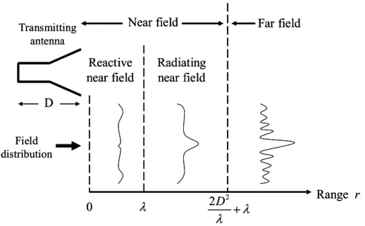
The exterior fields of a transmitting antenna can be divided into near-field and far-field regions as shown in Fig. 2.1 [14], [19]. The near-field region is further divided into two sub-regions, the reactive and radiating near field. In the reactive near field, energy is stored in the electric and magnetic fields very close to the transmitting antenna instead of radiating from the source. The near-field region is commonly taken to extend about λ π2 from the surface of the antenna. However, with the experience of

near-field measurement, it indicates that a distance of one wavelength ( λ ) determines a more reasonable outer boundary to the reactive near field. Once the distance from the

transmitting antenna is more than one wavelength, the electric and magnetic fields tend

to propagate predominantly in phase, but do not exhibit a plane-wave characteristic

(exp ikr r ) until they reach the far-field region. This propagation region between the

( )

reactive near field and the far field is called the radiating near field.

D

0 λ ^2D2 λ

λ ⁺

Range r

Field distribution

Reactive near field

Radiating near field

Transmitting antenna

Near field Far field

D

0 λ ^2D2 λ

λ ⁺

Range r

Field distribution

Reactive near field

Radiating near field

Transmitting antenna

Near field Far field

Fig. 2.1 Antenna near and far field regions.

The far-field region extends to infinity and the direction of electric field, magnetic

field and propagation are perpendicular among one another in this region. The inner

radius of the far field can be estimated from the general free-space integral for the

vector potential and is typically set at2D² λ λ+ . Notice that the added λ covers the possibility of the maximum dimension D of the antenna being smaller than a

wavelength. In other words, the so-called Rayleigh distance 2D² λ is measured from

the outer boundary of the reactive near field of the antenna.

2.3 Antenna Coupling versus Longitudinal Displacement

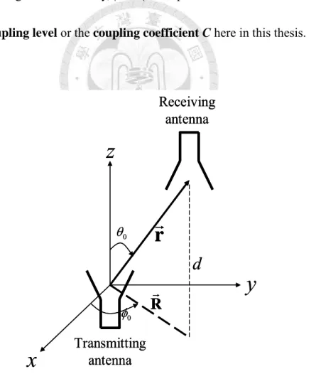
Consider a receiving antenna placed in the near field of a transmitting antenna as

depicted in Fig. 2.2. The incident and emergent waveguide mode coefficients for the

transmitting (receiving) antenna are aT and bT (aR and bR) respectively. Referring to [15],

the coupling quotient between the transmitting and receiving antennas is defined as

bR/aT. It can be interpreted as the signal coupled into the receiving antenna when a unit

signal is fed into the transmitting antenna, which is identical to the definition of the

forward transmission coefficient of the scattering parameters S21, when the transmitting

and receiving antennas and the region in between are considered as a two-port network.

Since we are more interested in the coupled power level, |bR/aT|² is used instead. It

means the amount of power accepted by the receiving antenna when a unit power comes

from the transmitting antenna. Mostly, |bR/aT|² is expressed in decibels and is referred to

as the power coupling level or the coupling coefficient C here in this thesis.

Transmitting antenna

Receiving antenna

x

y z

r G

R G

d

θ0

φ0

Transmitting antenna

Receiving antenna

x

y z

r G

R G

d

θ0

φ0

Fig. 2.2 Arbitrarily oriented receiving antenna in the near field of a transmitting antenna.

2.3.1 Spherical Wave Expansions for the Coupling Coefficient

The coupling quotient between the transmitting and receiving antennas can be

written as [15]

R R R

( ) ( )

T i

x y

T K k z

f f

b C

e dk dk

a k k

⋅

<

= − ∫∫ − ⋅ ^{k k}

^{k r} (2.2)

where

k = xk ˆ

_x

+ yk ˆ

_y

+ zk ˆ

_z is the propagation vector, and

k = k = 2 π λ

with λ the free-space wavelength.

r = xx yy zd ˆ + ˆ + ˆ = + R zd ˆ

t to the transmitting antenna.

alized vector far-

is the position vector of the

rece and

transmitting antennas, respectively. CR is a mismatch constant defined as iving antenna with respec

φ

θ φ_T

T f

f + ˆ are the norm

φ

θ φ

θ _{R R}

R f f

f = ˆ + ˆ

field patterns for the receiving and

T θ f = ˆ

( ¹

^RFeed

)

R

R L

C Z

= η

− Γ Γ

(2.3) where η is the intrinsic impedance of free space, ZRFeed is the characteristic impedance of the feed waveguide of the receiving antenna, and ΓR, ΓL are the reflection coefficients of the feed waveguide when looking into the receiving antenna and its passive load,

respectively. The derivation of (2.2) is done by Yaghjian [15] and shown in Appendix 1.

Note from (2.2) that the coupling quotient is a function of the position vector r.

The double integral in (2.2) is taken over the transverse components of propagation

vector dkx and dky, and the inner product of the two vector far-field patterns in the

integrand represents the interaction between the transmitting and receiving antennas.

The integral interval K < k means that only the propagating waves are integrated, which

corresponds to the real part of the complex power.

Applying the Laplacian operator ∇² to (2.2) yields

( ) ( )

( ) ( ) ( )

2 2

2

i

R T

R R

x y

T K k z

R T i

R

x y

K k z

f f

b C

e dk dk

a k k

f f

C k e dk dk

k k

⋅

<

⋅

<

− ⋅ ⎡ ⎤

∇ = − ⎣ ∇ ⎦

= − − ⋅ −

∫∫

∫∫

k r

k r

k k

k k

(2.4)

Recasting (2.4) and we have

(

^{2 2}

)

^R

⁰

T

k b

∇ + a =

(2.5) which means that the coupling quotient satisfies the scalar Helmholtz equation. As a

result, the coupling quotient can be expanded by linear combination of the elementary

wave functions, and the most general form is a summation over all possible values of m

and n [16], written as (see Appendix 2)

( )¹

( ) (

0

)

⁰

0

cos

n m im

R

nm n n

n m n

T

b B h k P e

a

θ

ϕ

∞

= =−

= ∑ ∑ ^r

(2.6) where r, θ0, and φ0 are the corresponding spherical coordinates of the position vector r. and are the spherical Hankel functions of the first kind and the associated

Legendre polynomials, respectively. Bnm are the spherical wave coefficients. Here, the

coupling quotient is expanded by a set of known basis which can be determined by

forward recurrence relations or obtained in Matlab and Mathematica databases, and

leaving only the spherical wave coefficients Bnm unknown.

( )1

hn P_n^m

Transmitting antenna

Receiving antenna

x

y z

d

z’

x’

y’

Transmitting antenna

Receiving antenna

x

y z

d

z’

x’

y’

Fig. 2.3 Rotated (primed) coordinate system with receiving antenna on the z’-axis.

Through the above series expansion method, the singularity that occurs when γ

approaches zero can be avoided, and the integration variables dkx and dky are changed to

be dθ0 and dφ0, resulting in a simpler double integral. To further simplify (2.6) and facilitate evaluation of Bnm, the coordinate system in Fig. 2.2 is rotated around the origin,

namely the phase center of the transmitting antenna, such that the phase center of the

receiving antenna lies on the z-axis of the rotated coordinate system as depicted in Fig.

2.3.

Therefore, in this new coordinate system

r = ˆzd

and θ0 = 0°. The relative orientation between the transmitting and receiving antennas can then be accounted for

simply by rotating the far-field patterns accordingly. In addition, it is known that the

associated Legendre polynomial P_n^m

(

cosθ₀

)

, for its argument being unity, is nonzero only when m = 0. Thus (2.6) can be rewritten as (2.7):

( )¹

( )

0

,

2

R T R

T n

b D D

d d

a

> + B h

n n

k

∞

=

= ∑

(2.7)

where DT and DR are the largest dimensions of the transmitting and receiving antennas,

respectively. The coupling quotient in (7) is now a function of the antenna spacing d

rather than the position vector r. The remaining work is to evaluate the unknown

spherical wave coefficients Bnm and Bn.

2.3.2 Evaluation of the Spherical Wave Coefficients

To evaluate Bnm and acquire Bn in (2.7), first we begin with (2.2), and let the

separation distance r approach to infinite. According to the Sommerfeld radiation

condition, (2.2) can be written as

( ) ² ( ) ( )

R R

b C

r f

a k

π

→ ∞

nts [17] and behaves as

ikr

R T

T r

i e

f r

→∞

∼ − ⋅ k k

(2.8)

On the other hand, as r the spherical Hankel function in (2.6) has an

approximation of large argume

⁽¹⁾

( ) ( )

¹

ikr n n

r

h kr i e

kr

+

→∞

∼ −

(2.9) Substituting (2.9) into (2.6), and compared with (2.8), we have

( ) ( ) ( )

1 0

0 0

2

( ) (cos )

ikr R

R R T

Tr

n ikr

im

n m

nm n

n m n

b e

r C i f f

a k

e

r

B i P e

kr

φ

π

θ

→∞

∞ +

= =−

= × − ⋅ ×

⎡ ⎤

= ⎢ − ⎥

⎣ ⎦

∑ ∑

k k

(2.10)

Clearly ,e^ikr kr can be canceled out. In a further step, we multiply both side of

(2.10) by P_n^m

(

cosθ0

)

e^-imφ0, and exploit the orthogonality relationships of those basis

functions as shown by Appendix 3, we have

( ) ( ) ( )

( ) ( ) ( )

⁰

2

0 0

0 0

2 1 !

2 !

cos sin

n

nm R

im m

R T n

i n n m

B C

n m

0 0

f f P e d d

π π

θ

⁻ φ

θ φ θ

+ −

= − ×

+

∫ ∫ − ⋅ ^{k k}

(2.11)

For m = 0, (2.11) reduces to

( )

( ) ( ) ( )

0

2 0

0 0 0

0 0

2 1 2

cos sin

n

n n R

R T n

B B C n i

f f P d d

0

π π

θ θ φ θ

= = − + ×

∫ ∫ − ⋅ ^{k k}

(2.12)

Given the 3D vector far-field patterns for both transmitting and receiving antennas

and the relative orientation, the associated inner product in the integrand of (2.12) could

readily be calculated. Please note that to evaluate Bn Yaghjian exploited an FFT

algorithm in [14] to convert the double integral into summations. In this work, a simple

numerical integration is adopted to calculate Bn directly from (2.12). Substituting Bn

thus obtained into (2.7) yields the desired coupling quotient. Although an infinite series

is needed based on (2.7) to compute the coupling quotient, it has been observed that the

series would converge with merely less than ten terms.

Furthermore, in the far-field Friis equation (2.1) p= ⋅e eˆ ˆ_{t R} ² indicates the polarization mismatch loss between two antennas, where and are unit vectors

representing the polarization of the electric field of the transmitting and receiving

antennas, respectively. In the proposed near-field formulation, the polarization

mismatch loss has also been consulted by the pattern inner product ˆ_t

e eˆ_R

R T

f ⋅ f since we

can always express f_R as θˆf_Rθ +ϕˆf_Rϕ and f_T as θˆf_Tθ +ϕˆf_Tϕ . Consequently, the

proposed formulation, in a sense, can be regarded as a near-field counterpart of the Friis

transmission formula.

2.3.3 Relative Orientations

To evaluate the inner product f_R⋅ f_T, the normalized far-field vector patterns( fR

and fT ) are transferred from the spherical coordinate system to the rectangular

coordinate system. Since there is often a relative orientation between transmitting and

receiving antennas, consider each antenna rotates about Z-axis as illustrated in Fig. 2.4.

We convert f f_φ, _θ from spherical coordinates into f f f_x, ,_{y z} in rectangular

coordinates by

sin cos cos cos cos sin

0 sin

x A A A

y A A A

z A

f f

f f

f

φ θ

φ θ φ

φ θ φ

θ

⎡ ⎤ ⎡ − ⎤

⎢ ⎥ ⎢ = ⎥ ⎡ ⎤ ⎢ ⎥

⎢ ⎥ ⎢ ⎥ ⎣ ⎦

⎢ ⎥ ⎢ − ⎥

⎣ ⎦ ⎣ ⎦

(2.13)

x

y z

k

θ

A

φ

A

k

z

K

x

y z

k

θ

A

φ

A

k

z

K

Fig. 2.4 A relative orientation of the receiving antenna in terms of spherical coordinate system

(

θ φA^, A

)

.

f , ,

After obtaining _x f f_{y z}, we can substitute it into (2.12) to compute the pattern

inner product, and further attain (2.7).

2.4 Antenna Coupling versus Transverse Displacement

In the preceding work, we evaluate the coupling coefficient versus the longitudinal

axis between the transmitting and receiving antenna. Mostly, in this situation the

coupling coefficient is larger than the scenario that the receiving antenna has an offset

(Δx, Δy) on a transverse plane and is separated from the transmitting antenna by d.

Typically this scenario is often our concern for application purpose.

The coupling coefficients are also obtained for this scenario. Consider the

transmitting antenna is located at the coordinate origin, while the receiving antenna

“scans” on a transverse plane with a constant antenna orientation. Fig. 2.5 shows the

receiving antenna located at an off-axis point A’ with transverse offsets (Δx, Δy) from

the on-axis point A. The transverse offsets can then be converted into the relative

orientation for the antennas.

1

2 2

1

tan

tan y x

x y

d φ

θ

−

−

⎧ Δ = ⎛ ⎜ Δ ⎞ ⎟

⎪ ⎝ Δ ⎠

⎪ ⎨ ⎛ Δ + Δ

⎪Δ = ⎜ ⎟

⎪ ⎜ ⎝ ⎟ ⎠

⎩

⎞

(2.14)

Given the tag antenna position A’(Δx, Δy, d) and the 3D patterns of the reader and

tag antennas, the associated coupling coefficient can be computed by rotating the 3D

patterns in accordance with the relative antenna orientation. Also, note that the antenna

spacing in the formula should be d’ instead of d.

x

y z

Δ x

Δ y

A

A’

d d ′

Transmitting antenna

Receiving antenna

(Δx, Δy, d) (0, 0, d)

x

y z

Δ x

Δ y

A

A’

d d ′

Transmitting antenna

Receiving antenna

(Δx, Δy, d) (0, 0, d)

Fig. 2.5 The receiving antenna has an offset (Δx, Δy) on the transverse plane normal to the separation axis.

2.5 Summary

In this chapter, we specify the near-field region discussed in this thesis. A simple

formulation has been presented for computing the coupling coefficients between two

antennas that are placed in the near field of each other and are arbitrarily oriented.

Although the formula is complicated to some extent, it could be regarded as a near-field

counterpart of the Friis transmission formula. Based on the proposed formula and

program, all the information we need to compute the near-field coupling coefficient are

the 3D radiation patterns of each antenna and their relative orientation.

Chapter 3

Comparisons between the Formulation and HFSS Simulation

3.1 Introduction

In order to verify the proposed formulation, three classic scenarios in the UHF band are considered in this chapter. The design frequencies of all the antennas are at 915 MHz. The associated coupling coefficients between the transmitting and receiving antennas are computed and compared to those simulated using Ansoft HFSS. Please note that, in the HFSS simulation, the quantity |S21|² is used for comparison, which is obtained by assuming port 2, namely the receiving antenna in our cases, being perfectly

matched to its load impedance. For consistency, this condition can be included in our formulation merely by setting ΓRL = 0. Also, it must be mentioned that according to the

condition in (2.7) the coupling coefficients can be computed only when the antenna

separation is larger than the mean value of the largest dimensions for the transmitting and receiving antennas. Therefore, d ≥ 85 mm is chosen in the following examples.

3.2 Side-by-Side, Parallel Half-Wave Dipoles

Consider two identical, y-directed half-wavelength dipole antennas, one of which is placed at the origin and the other on the z-axis with a separation d. The former is

chosen as the transmitting antenna, while the latter is the receiving antenna. Since it is not difficult to derive the normalized vector far-field pattern of an ideal y-directed half-wavelength dipole based on its well-known z-directed counterpart, they are given as

2 2

sin sin

cos 2

cos sin 1 sin sin

f

_θ

π θ ϕ

θ ϕ

θ ϕ

⎛ ⎞

⎜ ⎟

⎝ ⎠

∝ −

(3.1)

2 2

sin sin

cos 2

1 sin sin cos f

_ϕ

π θ ϕ

θ ϕ ϕ

⎛ ⎞

⎜ ⎟

⎝ ⎠

∝ −

(3.2)

Substituting (3.1) and (3.2) into (2.12) yields the desired spherical wave coefficients Bn. The computed coefficients Bn diminishes significantly for higher order terms when n > 7 leading to fast convergence of (2.7). In the HFSS simulation, the configuration of the dipole is shown in Fig 3.1, and the corresponding patterns at 915 MHz are shown in Fig 3.2.

x

y z

Dipole 156

mm

2 mm

x

y z

Dipole 156

mm

2 mm

Fig. 3.1 Geometry of the HFSS simulated dipole.

(a) (b)

0

90

180 270

-10 dB

simulated E-phi simulated E-theta

10 dB 0

90

180 270

-10 dB

simulated E-phi simulated E-theta

10 dB

(a) (b)

0

90

180 270

-10 dB

simulated E-phi simulated E-theta

10 dB 0

90

180 270

-10 dB

simulated E-phi simulated E-theta

10 dB

Fig. 3.2 Simulated radiation patterns of the dipole at 915MHz.

(a) x-z plane and (b) y-z plane.

50 100 150 200 250 300 350 400

-40 -35 -30 -25 -20 -15 -10 -5 0

x

y z

x

y z

Coupling Coefficient (dB)

Antenna Separation d (mm)

calculated coupling coefficient (by close-form pattern expression)

simulated S21 (by HFSS)

Fig. 3.3 Coupling coefficient versus antenna separation for polarization-matched dipoles.

The near-field coupling coefficient as a function of antenna spacing d computed by the proposed method and those obtained via HFSS are depicted in Fig. 3.3. Excellent agreement can be observed verifying the proposed formulation.

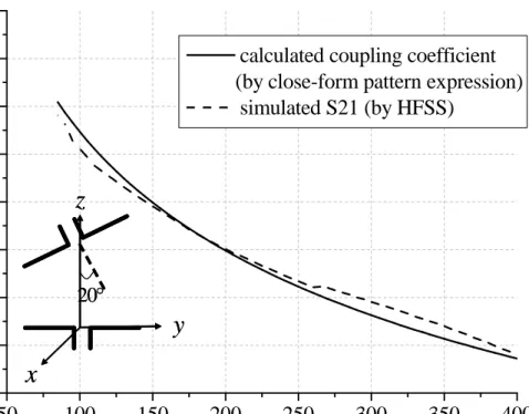
3.3 Side-by-Side, Polarization-Mismatched Half-Wave Dipoles

In the preceding subsection, the two dipoles are polarization matched corresponding to the best case in a two-dipole system. However, in most cases, they are arbitrarily oriented. Besides, to demonstrate the capability of our method, a scenario

having polarization-mismatched dipoles is also considered. In the current case, the receiving dipole lying on the y-z plane is rotated by 20° around its phase center. This

can be accounted for in our formulation simply by transforming the coordinate system of the vector far-field pattern of the receiving dipole accordingly. Using (2.13),

θA andφ_A defined in Fig. 2.3 are 20° and 90°, respectively. Accordingly the corresponding rectangular components of the receiving antenna are

cos 20 sin 20

xR R

yR R

zR R

f f

f f

f f

φ

θ

θ

⎧ = −

⎪ = ° ⋅

⎨ ⎪ = − ° ⋅

⎩

(3.3)

Likewise, Bn thus obtained diminishes significantly for n > 9 leading to fast convergence of (2.7). The coupling coefficients thus obtained are plotted in Fig. 3.4.

One can see that the coupling coefficients are smaller here than in the preceding case because of the polarization mismatch between the two dipoles.

50 100 150 200 250 300 350 400 -40

-35 -30 -25 -20 -15 -10 -5 0

calculated coupling coefficient (by close-form pattern expression)

simulated S21 (by HFSS)

20°

x

y z

20°

x

y z

Coupling Coefficient (dB)

Antenna Separation d (mm)

Fig. 3.4 Coupling coefficient versus antenna separation for polarization-mismatched dipoles.

3.4 Polarization-Matched Square Loop and Half-Wave Dipole

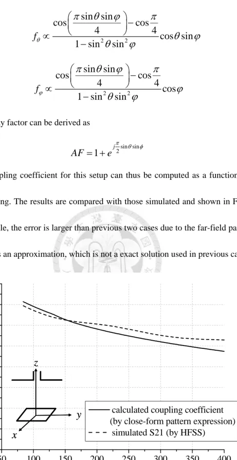
Here, a square loop antenna having its perimeter equal to a wavelength is used to replace the transmitting dipole in Section 3.2. The loop antenna is centered at the origin with the loop lying on the x-y plane and oriented in such a way that the resultant polarization is aligned with the y-directed receiving dipole. In the HFSS simulation, the structure of the square loop antenna and the patterns are shown in Fig 3.5 and Fig 3.6, respectively.

x y z

Square loop

89 mm

2 mm

x y

z

Square loop

89 mm

2 mm

Fig. 3.5 Geometry of the HFSS simulated square loop.

(a) (b)

0

90

180 270

-10 dB

simulated E-phi simulated E-theta

10 dB

0

90

180 270

-10 dB

simulated E-phi simulated E-theta

10 dB

(a) (b)

0

90

180 270

-10 dB

simulated E-phi simulated E-theta

10 dB

0

90

180 270

-10 dB

simulated E-phi simulated E-theta

10 dB

Fig. 3.6 Simulated radiation patterns of the square loop antenna at 915MHz.

(a) x-z plane and (b) y-z plane.

We observe that the simulated pattern in the y-z plane is doughnut-shaped, while the x-z plane pattern is omni-directional with a slightly shaking at ±90°. This circumstance indicates that its normalized co-polarized component of the far-field pattern can be represented as an array composed of two parallel dipoles a quarter wavelength apart. Consequently, the radiation patterns of the square loop can be approximated using the principle of pattern multiplication with the element factor

2 2

sin sin

cos cos

4 4

cos sin 1 sin sin

f

_θ

π θ ϕ π

θ ϕ

θ ϕ

⎛ ⎞ −

⎜ ⎟

⎝ ⎠

∝ −

(3.4)

2 2

sin sin

cos cos

4 4

1 sin sin cos f

_ϕ

π θ ϕ π

θ ϕ ϕ

⎛ ⎞ −

⎜ ⎟

⎝ ⎠

∝ −

(3.5)

while the array factor can be derived as

sin sin

1

^j2

AF e

π θ φ

= +

(3.6) The coupling coefficient for this setup can thus be computed as a function of the antenna spacing. The results are compared with those simulated and shown in Fig. 3.7.

In this example, the error is larger than previous two cases due to the far-field pattern of square loop is an approximation, which is not a exact solution used in previous cases.

50 100 150 200 250 300 350 400

-40 -35 -30 -25 -20 -15 -10 -5 0

x

y z

x

y z

calculated coupling coefficient (by close-form pattern expression)

simulated S21 (by HFSS)

Coupling Coefficient (dB)

Antenna Separation d (mm)

Fig. 3.7 Coupling coefficient versus antenna separation for polarization-matched square loop and dipole.

3.5 Summary

In the previous three scenarios, the agreement between the computed results and those simulated by HFSS indicates that the proposed method can be utilized to determine the near-field coupling coefficient as the relative orientation, the antenna spacing, and the far-field patterns of the transmitting and receiving antennas are known.

Chapter 4

Application in Near-Field UHF RFID System

4.1 Introduction

A RFID system is a spontaneous wireless data collection technology with a long history [18]. Depending upon their operating principle, RFID systems are classified into three categories: passive, semi-passive, and active. A passive RFID system is the least complex and cheapest, hence widely used for many applications. Without a power supply of a passive tag its own, the required energy to turn on the tag chip depends upon the electromagnetic field coupling from the reader. Accordingly, two different coupling techniques are further categorized: near-field coupling and far-field coupling.

Low frequency (LF, 125-134 kHz) and high frequency (HF, 13.56 MHz) RFID systems are short-range systems based on near-field coupling. On the other hand, Ultra-high frequency (UHF, 860-960 MHz) and microwave (2.4 GHz and 5.8 GHz) RFID systems are typically long-range systems based on far-field coupling. LF and HF RFID systems have been deployed in the market for many commercial applications.

However, the larger size of the antennas used in the LF/HF band systems confines their further development. Thus, it is straight forward to reduce antenna size by designing the system in a higher frequency band, such as the UHF band. In addition, the near-field

UHF RFID systems have other superiorities, including higher data rate, and lower manufacturing cost, making them suitable for item-level tagging.

The near-field UHF RFID system is composed of a reader and a tag just as in the ordinary RFID systems. The simplified system architecture is depicted in Fig. 4.1. The power generated by the reader circuitry Preader is transferred to the reader antenna, and then acquired by the tag antenna through near-field coupling. The power absorbed by the tag chip Pchip can be expressed as [19]

chip reader reader chip

P = P × τ × × C τ

(4.1) where τreader and τchip are the impedance mismatch coefficients of the reader and tag between the front-end circuitry and the associated antenna, respectively. They can be expressed as

2

2

1 ,

1 ,

T S

reader t t

T S

C R

chip R R

C R

Z Z Z Z

Z Z

Z Z

τ

τ

^∗

⎧ = − Γ Γ = −

⎪ +

⎪ ⎨

⎪ = − Γ Γ = −

⎪ +

⎩

(4.2)

Please note that since both the impedances of tag and chip are complex, we use a modified power wave reflection coefficient proposed by Kurokawa [20]. Equation (4.2) also indicates that the maximum power transfer occurs at conjugate impedance match between both components.

ZS

Z^T RFID

reader

RFID tag chip

Z^R Z^C

Coupling ZS

Z^T RFID

reader

RFID tag chip

Z^R Z^C

Coupling

Fig. 4.1 Simplified architecture of near-field RFID systems.

C is the coupling coefficient between the reader and tag antennas. With the aid of the proposed formulation (2.7), (2,12), the coupling coefficient C can be readily calculated.

To verify the results by experiment, a near-field UHF RFID system is implemented in this chapter. In Section 4.2, we present a broadband square loop array with a back- reflector and it is used as the reader antenna. In Section 4.3, two different tag antenna designs [21], [22] are used individually in the system. We compared a series of experiments with the proposed formulation in Section 4.4. The measurement results are in good agreement with those computed by the proposed method and those simulated by HFSS as well. Furthermore, some factors are found to be crucial for improving the power coupling level in Section 4.5. For practical applications, such as Point of Sale (POS), the proposed formulation is capable of determining the near-field read range and the read reliability, which is introduced in Section 4.6. Finally, we summarized the measured results and findings in Section 4.7.

4.2 Reader Antenna

Typically, a loop antenna is favorable for a near-field reader antenna. However, the square loop with perimeter of a wavelength demonstrated in Section 3.4 is not an appropriate design due to poor concentration of power. Therefore, we develop a loop array with back-reflector to aggregate the radiated power.

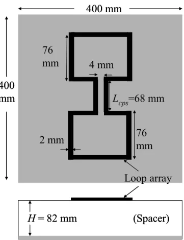
The geometry of the proposed reader antenna for the near-field UHF RFID system is shown in Fig. 4.2, and the photographs are shown in Fig 4.3. Two printed square loop antennas, of which the perimeters are equal to a wavelength, are back-to-back connected by a coplanar strip (CPS) of length Lcps. The two arms of the CPS are connected respectively at their midpoints to the inner and outer conductors of the feeding coaxial cable. The coaxial cable is fed from the direction normal to the antenna plane. Although a balun could be added to slightly improve the radiation performance, the proposed design directly fed via a coaxial cable can still provide satisfactorily higher gain and well-shaped radiation pattern. As one may expect, the design radiates bi-directionally;

however, most RFID reader antennas require unidirectional radiation pattern. To produce unidirectional radiation pattern and further increase the antenna gain, an electrically large, planar conducting sheet is utilized as a back reflector for the loop array as shown in Fig. 4.2 The spacing H between them is set to be approximately a quarter wavelength in free space.

2 mm 76 mm 76

mm

L

_cps

=68 mm 4 mm

400 mm

400 mm

H = 82 mm (Spacer) Loop array

2 mm 76

mm 76

mm

L

_cps

=68 mm 4 mm

400 mm

400 mm

H = 82 mm (Spacer) Loop array

Fig. 4.2 Geometry of two-element square loop array with a back reflector.

(a) (b)

Fig. 4.3 Photographs of two-element square loop array with a back reflector.

A prototype antenna designed around 915 MHz was fabricated on an FR-4 substrate with dielectric constant εr = 4.4 and thickness h = 0.6 mm. A copper sheet of dimensions 400×400 mm² is used as the back reflector and placed at a distance H = 82

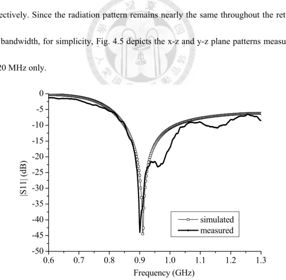
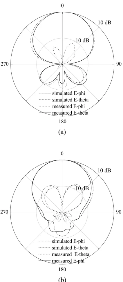
mm from the loop array. Throughout the design process, simulations are carried out on HFSS. The simulated and measured input return losses of this antenna are shown and compared in Fig. 4.4. We can find that the design is well matched within a wide frequency range, and the measured 10-dB return loss bandwidth is 19.1% (848-1022 MHz). The peak gains measured at 920 MHz and 930 MHz are 10.2 and 10.1 dBi, respectively. Since the radiation pattern remains nearly the same throughout the return loss bandwidth, for simplicity, Fig. 4.5 depicts the x-z and y-z plane patterns measured at 920 MHz only.

0.6 0.7 0.8 0.9 1.0 1.1 1.2 1.3

-50 -45 -40 -35 -30 -25 -20 -15 -10 -5 0

simulated measured

|S11| (dB)

Frequency (GHz)

Fig. 4.4 Simulated and measured input return losses of the reader antenna.

0

90

180 270

-10 dB

simulated E-phi simulated E-theta measured E-phi measured E-theta

10 dB

(a)

0

90

180 270

-10 dB

simulated E-phi simulated E-theta measured E-theta measured E-phi

10 dB

(b)

Fig. 4.5 Simulated and measured radiation patterns of the proposed reader antenna at 920MHz. (a) x-z plane and (b) y-z plane.

4.3 Tag Antennas

Passive tags utilize the coupled energy from a reader to power up the chip circuit.

To have a superior power transfer between the tag antenna and the chip, the input impedance must be conjugate matched to the chip impedance, which is highly capacitive generally. The capacitive reactance of chip impedance makes the matching task become difficult between tag antenna and chip. Thus the design guidance of tag antennas is miniaturized as well as a well-coupled power. Two different tag antenna designs, referring to [21] and [22] are implemented. Each of them is used in our near-field experiment setup.

4.3.1 Folded Dipole with a Closed Loop

The first one is a folded dipole with a closed loop [21] whose main advantage is its tunable input impedance to achieve conjugate match for various commercial tag chips.

A prototype antenna design at 915 MHz is depicted in Fig. 4.6, and the photograph of the antenna, of which the total antenna area is 64.4 × 27.6 mm², is shown in Fig. 4.7.

Please note that, to facilitate measuring the coupling coefficient through the vector network analyzer (VNA), the antenna is designed for 50 Ω instead of being conjugate

matched to the highly capacitive tag chips and is fed by a section of CPS connected to a balun connected to the coaxial cable. This additive balun degrades the

25.76 mm

27.6 mm

64.4 mm

9.2 mm 28.52

mm

Balun

Fig. 4.6 Geometry of the folded dipole antenna.

Fig. 4.7 Photograph of the folded dipole antenna.

pattern of the tag antenna inevitably, which will be stated and discussed at Section 4.3.3.

The proposed folded dipole was fabricated on the FR-4 with thickness of 0.6 mm.

The simulated and measured return losses of the folded dipole with the Balun are shown and compared in Fig. 4.8, and the radiation patterns of x-z plane and y-z plane are