國立臺灣大學工學院土木工程學系 碩士論文
Department of Civil Engineering College of Engineering National Taiwan University
Master Thesis
懸浮泥砂之對流、擴散及隨機運動機制之探討
A probabilistic description of suspended sediment transport:
advection, diffusion and random movement
吳棕翰 Tsung-Han Wu
指導教授:蔡宛珊 教授 Advisor: Christina W. Tsai, Ph.D.
中華民國 105 年 7 月
July, 2016
誌謝
時光飛逝,很快的兩年的時間一下就過去了,和研究所同學一起面對艱難的 課業使我們在這短短的兩年培養出堅韌的革命情感,也幸運的完成了這艱難的目 標。首先我要感謝我的指導教授蔡宛珊老師,老師在研究的方向給予我們很大的 自由,且以美式教育般的方式鼓勵我們,以讚美代替責罵,因材施教。在論文方 面老師要求我們以英文撰寫,並且不嫌麻煩的為我們檢查論文,使我的英文寫作 能力有所進步。也要謝謝 914 的成員們,因為有你們讓我的研究所生活更精采,
我的研究好夥伴阿谷和葉小胖還有學長隆成,真的很幸運可以和你們一起研究和 學習。也非常謝謝學弟妹家昕、氣祥在研究和課業的幫助,你們讓 914 充滿了活 力。在這裡還要特別感謝學姊毓茹和學妹家昕,因為有你們的幫助,我的「英文 論文」才得以順利完成。感謝卡門的阿霞、阿宜、王董志中,讓我們蔡門可以常 常幫助你們做實驗,並且更了解卡老師的研究。也謝謝水利智者品慶,常常提出 很有見解的意見,讓我獲益良多。潔晰卡常常提供好吃的食物真是太感謝你啦,
讓我們不會研究過度而血糖降低。工具人之首富建真的是太罩了,感謝你幫忙許 多事情,因為太多了我一時也無法以一一列出。最後要感謝我的父母,謝謝你們 在我求學階段的照顧,可以不用煩惱其他事情。最後還是要引用一下經典名句,
需要感謝的人實在太多了,就感謝天吧!
中文摘要
泥砂運輸與人類的生活息息相關,例如橋墩沖刷、水質估計等等,故泥砂運 輸的研究是一直以來都是一個很重要的議題。泥砂顆粒在水中除了隨著水流方向 運動之外,也會因為受到紊流的影響而向周圍不規則擴散,此外,其運動的行為 可以馬可夫鏈(Markov chain)來近似,因此本研究將泥砂顆粒的運動視為一個隨機 過程。本文以力學原理結合序率方法(Stochastic method)來模擬泥砂顆粒在水中的 運動軌跡,亦即增強隨機微分方程中的物理性質,使之更貼近自然情形。
為模擬泥砂顆粒的運動行為,本文以朗之萬方程(Langevin equation)為原型所 推導出的隨機擴散粒子追蹤模型(Stochastic Diffusion Particle Tracking Model)呈現 顆粒運動因紊流而造成的不確定性。其中,隨機擴散粒子追蹤模型主要包含兩種 基本元素:平均漂移項(Mean drift term),即為顆粒隨著水流方向運動;紊流項 (Turbulence term),即顆粒受到紊流作用而有不規則的運動,也稱為布朗運動 (Brownian motion),係利用維納過程(Wiener process)來模擬。
本研究利用隨機擴散粒子追蹤模型來模擬在一般流況下泥砂顆粒的運動軌跡,
分別使用兩種隨機擴散粒子追蹤模型: 單顆粒粒子追蹤模型(One-particle Particle Tracking Model)和雙顆粒粒子追蹤模型(Two-particle Particle Tracking Model)去模 擬。其中,雙顆粒粒子追蹤模型比單顆粒粒子追蹤模型多考慮了顆粒在距離相近 時候的變化,因為大尺度的渦流(Large scale turbulence)的關係可能使彼此相近的顆 粒具有相似的隨機運動。另外,以巨觀的角度去觀察顆粒整體的運動,可以計算 出水中的泥砂濃度,且因為泥砂顆粒受到紊流擾動的影響,使得泥砂的濃度也具 有不確定的變化。因此本文呈現顆粒軌跡和泥砂濃度的平均值和標準差來表示泥 砂顆粒在水中的不確定性。本研究首先和實驗資料比對單顆粒和雙顆粒粒子模型 所估計的濃度以驗證模型的可行性,最後使用此模型分別探討層流流場中和紊流 流場中顆粒隨機運動的情形,結果顯示在紊流流場中顆粒的隨機運動比較明顯,
因此在高雷諾數(Reynolds number)的流場中估計泥砂濃度時,應考慮漩渦對泥砂顆 粒所造成的隨機變化,並給予濃度變動範圍較為恰當。此外,泥砂顆粒運動具有 馬可夫特性也在本文中證實。然而,如本文結果所顯示,泥沙顆粒的移動距離卻
有再懸浮的現象可能導致泥砂擴散為反常擴散(non Fickian diffusion or anomalous diffusion)。
關鍵字:隨機微分方程、序率模式、顆粒軌跡模型、泥砂運動、雙顆粒模型、馬 可夫特性、反常擴散
ABSTRACT
Sediment transport is an important issue for human. It is closely related to human society, such as bridge scour and water quality. A sediment particle in flow not only follows the flow direction, but also diffuses through the surrounding water due to turbulence. Markov chain is used to approach the movement of sediment particles.
From this perspective, particle movement is regarded as a stochastic process in our study; moreover, the proposed models simulate particle trajectories based on stochastic methodologies and physical mechanisms, underscoring mechanics in the stochastic differential equation.
To simulate sediment particle movement, the stochastic diffusion particle tracking model (SD-PTM) has been derived from the Langevin equation, which is able to show the random characteristics of sediment movement. SD-PTM has two basic elements, the mean drift term and the turbulence term. One of the particle characteristics, the mean drift term, is that particles follow the flow direction; another one is called the turbulence term that describes random behaviors caused by turbulence diffusion. This movement is known as Brownian motion. In general, the diffusion movement is modeled by the Wiener process.
The aim of this study is to simulate sediment particle trajectories under the normal flow condition by the SD-PTMs, one-particle PTM and two-particle PTM. The difference between the single particle model and the paired particle model is that the paired particle model accounts for large eddy turbulence. In other words, the paired particles may have similar random movement if the locations of particles are in the immediate vicinity of each other. Besides, to observe assemblage of particles’ motion in the macroscopic manner, the sediment concentrations can be estimated. Moreover,
sediment concentrations involve the property of uncertainty on account of sediment particles’ stochastic trajectories. Therefore, to demonstrate such uncertainty of sediment particles, the ensemble means and ensemble standard deviations of sediment trajectory as well as concentrations are presented in the study respectively. The proposed models are validated against experimental data by ensemble mean velocity and sediment concentrations. Moreover, this study also discussed the random movement of sediment particles under various flow conditions, laminar cavity flow and fully developed turbulent open channel flow. Results show that the random movement of sediment particles is significant in turbulent flow. Thus, it is appropriate to consider the fluctuation of sediment concentrations under high Reynolds number flow conditions.
Besides, the Markovian property of the PTMs is validated in our study. However, the variance of particle displacement and time are not a linear proportion as the result.
Resuspension of sediment particles may cause particle movement to be anomalous diffusion.
Keyword: stochastic differential equation, stochastic model, particle tracking model, sediment transport, two-particle model, Markovian property, anomalous diffusion.
CONTENTS
口試委員會審定書 ... #
誌謝 ...i
中文摘要 ... ii
ABSTRACT ...iv
CONTENTS ...vi
LIST OF FIGURES ...ix
LIST OF TABLES ...xi
Chapter 1 Introduction ... 1
1.1 Problem statement ... 3
1.2 Research Hypotheses ... 4
1.3 Objectives of Study... 7
1.4 Overview of Thesis ... 7
Chapter 2 Literature Review ... 8
2.1 Stochastic Methods ... 8
2.1.1 The Eulerian model ... 9
2.1.2 The Lagrangian model ... 10
2.2 Pickup Probability ... 11
2.3 Turbulent diffusion and dispersion ... 15
2.4 Summary ... 17
Chapter 3 Stochastic Theories ... 18
3.1 Markov Process ... 18
3.2 Brownian Motion ... 19
3.4 Numerical Approximation for Stochastic Differential Equations ... 23
3.5 Summary ... 27
Chapter 4 Development of Stochastic Particle Tracking Model of Suspended Sediment Transport ... 28
4.1 Introduction... 28
4.2 Model Assumptions ... 30
4.3 Model Development ... 31
4.3.1 Stochastic Diffusion Model – One-Particle Particle Tracking Model. 31 4.3.2 Stochastic Diffusion Model – Two-Particle Particle Tracking Model 33 4.4 Determination of Hydraulic Parameters in Open Channel Flow ... 36
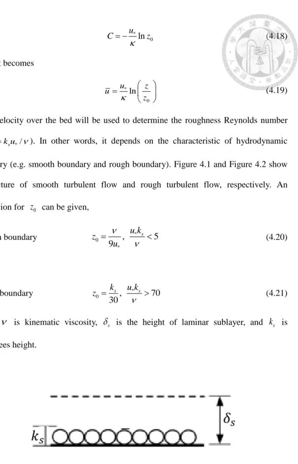
4.4.1 Velocity Profile ... 36
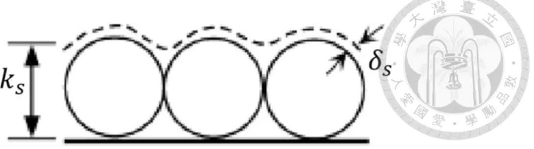
4.4.2 Particle Settling Velocity ... 39
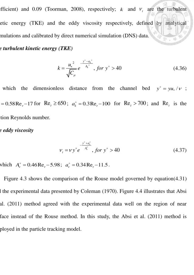
4.4.3 Diffusion Coefficient ... 41
4.4.4 Re-suspension Mechanism ... 46
4.5 Simulation Results ... 48
4.6 Summary and Conclusions ... 54
Chapter 5 Application of The Stochastic Particle Tracking Model ... 56
5.1 Introduction... 56
5.2 Case study of validating with experimental data ... 57
5.3 Case study of particle movement under two-dimensional laminar flow conditions ... 64
5.4 Case study of particle movement under fully developed uniform channel flow ... 68
5.5 Summary and Conclusions ... 74
6.1 Summary and Conclusions ... 77
6.2 Recommendations for Future Research ... 78
REFERENCE ... 79
APPENDIX ... 85
LIST OF FIGURES
Figure 1.1 Flow chart of two-particle PTM ... 6 Figure 2.1 The classic turbulence energy spectrum versus to length scales for the open channel flow (Roberts and Webster, 2002). ... 16 Figure 3.1 Simulation of 3000 samples of the Wiener process ... 21 Figure 3.2 Comparing with Weak solution, strong solution emphases the information of path ... 26 Figure 3.3 Ensemble mean of strong solution and weak solution ... 27 Figure 4.1 Turbulent flow under the condition of the smooth bed boundary (modified by MIT note). ... 38 Figure 4.2 Turbulent flow under the condition of the rough bed boundary (modified by MIT note). ... 39 Figure 4.3 Comparison between vertical distribution of suspended sediment diffusion coefficient and experimental data (Tsujimoto, 2010). ... 45 Figure 4.4 Comparison of different sediment suspended diffusion model. ... 45 Figure 4.5 The conservation of forces acting on individual sediment particles in bed load (Wu and Chou, 2003). ... 47 Figure 4.6 The condition for incipient motion of sediment particles is that the upward velocity of turbulent eddies w exceeds particles’ settling velocity ws (modified from Chen and Chew, 1999 and Bose and Dey, 2013). ... 47 Figure 4.7 The averaged particle correlation versus relative time ... 50 Figure 4.8 Sediment particles released from original by the one-particle PTM and two-particle PTM at time 0.1, 0.5, 1s, respectively ... 51
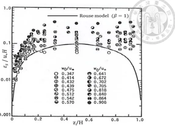
one-particle PTM and two-particle PTM ... 52 Figure 4.10 The correlation with z direction of different two sediment particles by the one-particle PTM and two-particle PTM ... 53 Figure 5.1 Comparison of mean particle velocities with NBS particle ... 58 Figure 5.2 Comparison of sediment concentration with Coleman measured data ( with diameter 0.105mm) ... 61 Figure 5.3 Sediment concentrations with on standard deviation by PTMs ... 61 Figure 5.4 Comparison of sediment concentration based on different released locations62 Figure 5.5 The variance of particle distance versus simulation time ... 63 Figure 5.6 The initial conditions of cavity problem ... 66 Figure 5.7 Validating flow field to Ghia et al. (1982) data ... 66 Figure 5.8 One of realizations of sediment particle released from original at time 0.02, 0.82, 1.6, 2.4, 3.2, 4, 4.8, 6s, respectively ... 67 Figure 5.9 The flow conditions of mean velocity (m/s), turbulent viscosity (m2/s) and TKE (turbulent kinetic energy (m2/s2)) ... 69 Figure 5.10 Comparison of Rouse model, Absi et al.(2011) model and the computed turbulent diffusivity ... 70 Figure 5.11 Ensemble mean of sediment particle trajectories (bold dot line) in 2-D flow71 Figure 5.12 Ensemble mean of sediment particles position in x, z-direction versus
simulation time ... 71 Figure 5.13 Ensemble variance of sediment particles position in x, z-direction versus simulation time ... 73 Figure 5.14 Ensemble sediment concentration ... 73 Figure 5.15 Sediment particle cloud in this channel flow ... 74
LIST OF TABLES
Table 1.1 Different types of model (modified from Yen, 2002) ... 4
Table 2.1 Summary of previous study ... 14
Table 3.1 Some parameters and initial conditions in the example ... 25
Table 4.1 Environment conditions in simple test and parameters in model ... 50
Table 5.1 The environmental conditions in the NBS flows ... 58
Table 5.2 Flow and sediment characteristics in Coleman (1986) ... 60
Table 5.3 The variance of sediment concentration by one-particle PTM and two-particle PTM ... 60
Table 5.4 The environmental conditions under laminar flow ... 65
Table 5.5 The CFD and sediment environmental conditions ... 70
Chapter 1 Introduction
Equation Chapter 1 Section 1
Irregular movement of particles owing to turbulence has been studied for many years. The drag force of turbulence fluid is a main factor that causes a particle to move randomly. For instance, hydraulic and environmental engineers have been highly concerned with sediment transport caused by turbulence. This is important for designing flow structure, water quality management and ecological environment. According to the particle properties, sediment particles can be classified into suspended load and bed load in flow. In general, a particle floating in the water column is classified as suspended load; bed load is defined as a particle moving near the bed. To study sediment transport, researchers and engineers used to concentrate on deterministic methods. There are many kinds of modeling approaches, such as the sediment-transport balance method and the sediment-divided method. Sediment-transport balance method is a method that offers the sediment balance equation derived from the sediment transport formula. In sediment-divided method, different particle movement is considered in order to decide whether a suspended load model or bed load model needs to be applied. The aforementioned models are mainly focused on particle concentration, i.e. particles in the Eulerian model seem to be presented by concentrations. However, more detailed information on trajectories of particles is preferred. Consequently, simulating sediment transport by Lagrangian models became more and more popular recently and were promoted in various fields such as hydraulics, marine, environment, economics, physics etc.( Man et al., 2007; Spivakovskaya et al., 2007; Oh and Tsai, 2010; Shah et al., 2011)
In order to study bed-load transport, Einstein (1942) established the foundation of
the applicability of probabilistic concepts. The entrainment probability function is innovated in sediment entrainment to bed load. In other words, stochastic properties have been suggested for the transport of sediment particles. A new viewpoint for stochastic models for sediment transport has been implemented ever since.
One category of the stochastic models is particle tracking models (PTM), also known as “Random walk models’’. This type of model can be treated as the transport of a constituent of large number of moving particles which can be simulated as discrete particles. Because of discrete particle characteristics, this stochastic process might be regarded as a Markov-process theory, meaning that particle position only depends on the present state instead of all past history. The PTM normally employs two terms: the mean drift term and random term. This stochastic transport model based on physical mechanisms are called the stochastic diffusion particle tracking model (SD-PTM), which is built on stochastic differential equations (SDE). Since SD-PTM, a type of Langevin equation is equivalent to the Fokker-Planck equation (FPE) derived from the advection-diffusion (ADE) equation for suspended sediment transport. The detail of model development will be introduced in chapter 4. In addition to this, turbulence flow plays an essential role because we are focused on the sediment transport in open channel flows. Unfortunately, turbulence in the open channel flows is not completely understood even in recently. Because of insufficient knowledge about turbulence, there exists uncertainty when attempting to modeling particle movement in flows. As such, the stochastic method is an appropriate way to describe the movement of sediment particles in this study.
1.1 Problem statement
The problem of sediment transport is closely related to the environment such as water quality, estuary improvement, environmental protection and estuary surrounding construction. In order to reach the above objectives, it is important to study the law of natural environment. With an enhanced understanding of sediment transport mechanisms, hydraulics constructions or engineering management can operate more effectively based on this scientific information. However, the natural environment is too difficult to simulate, as it involves multiple interacting factors. In other words, it is impossible to have complete information on all the factors in the natural process.
Moreover, sediment motion in the flow and eddies are a complex process, which can be regarded as a stochastic process. Most sediment transport models such as ADE or the Exner equation are deterministic models, meaning that if a model with the same input(s) will yield the same results. These deterministic models simplify the uncertain variables (e.g. sediment properties, and flow discharge) to deterministic values and neglect the irregular eddy effect. Stochastic models for complicated and random natural process are thus developed. These stochastic methods such as uncertainty analysis that considers uncertainties incurred in data by considering their probability of occurrences. Yen (2002) discussed the hydraulic problems with stochastic perspectives, which can be briefly summarized as follows.
Input System Output
Deterministic Deterministic Deterministic
Deterministic Stochastic Stochastic
Stochastic Deterministic Stochastic
Stochastic Stochastic Stochastic
Table 1.1 Different types of model (modified from Yen, 2002)
In this study, we consider the stochastic model-- SD-PTM to describe sediment particle movement in the open channel flows. A different concept of SD-PTM, two-particle PTM, is proposed by Spivakovskaya and Heemink (2006). Unlike traditional SD-PTM, the two-particle PTM suggested that the behavior of sediment particles caused by turbulence flow is correlated in space. Therefore, to more comprehensively model sediment particles, it is desirable to develop the two-particle PTM considering the effect of spatial correlation of particle behavior.
1.2 Research Hypotheses
Motion of sediment particles caused by turbulence is an irregular motion, which is difficult to describe exactly. This study raises two main hypotheses in the PTMs.
Markovian property
Sediment particles in open channel flows are poorly understood because of its random motion. Therefore, sediment particle motions are regarded as a memoryless stochastic process. The memoryless behavior is called as Markovian property. Based on
this, the FPE is used to describe particles’ movement. In the other words, sediment particles relates to the present state rather than the previous state.
Fickian law
Turbulent diffusivity plays an important role in the high Reynolds number flow.
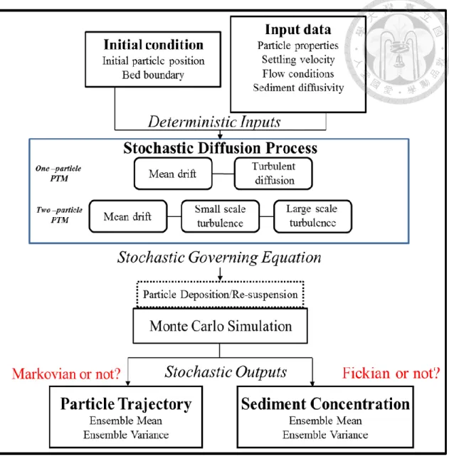
For instance, in turbulent flow, the effect of turbulence is more significant than that of the molecular diffusion. As will be introduced in chapter 4, turbulent diffusion is also considered as some form of random motion. The behavior of turbulence flow is analogous to Fickian diffusion. In Fickian law, the variance of particles displacement is defined to be linearly proportional to time. Figure 1.1 presents the flow chart of the PTMs. The difference between one-particle and two-particle PTMs is in the stochastic diffusion process. The two-particle PTM emphasizes the inter-particle relationship.
Figure 1.1 Flow chart of two-particle PTM
1.3 Objectives of Study
This study is intended to develop a refined stochastic diffusion particle tracking model for sediment transport in open channel flows to estimate sediment concentrations.
The main objectives are
i. to incorporate a more sophisticated turbulent diffusivity formula and a recently developed mechanism of re-suspension into the proposed stochastic particle tracking model;
ii. to simulate the movement of sediment particles under various flow conditions;
iii. to verify the proposed model by comparing the quantified sediment concentrations and velocity with experimental data;
iv. to compare and discuss the difference of the concentration fluctuations by proposed one-particle and two-particle models.
1.4 Overview of Thesis
This thesis includes two main hypotheses which are previously defined. Chapter 2 is a literature review about different opinions of quantitative sediment particles, and the important hydraulics parameters to the proposed models. In chapter 3, the foundation of stochastic theories and numerical schemes are presented. Chapter 4 is the development of the SD-PTM, including the derivation of SD-PTM from ADE and the equivalent equation, FPE, as well as the definition of hydraulics parameters. Chapter 5 demonstrates three applications by the proposed models with comparison of experimental data and the various flow field data, respectively. Lastly, Chapter 6 supplies a summary of the findings, contributions, and recommendations for future
Chapter 2 Literature Review
Equation Chapter (Next) Section 1
2.1 Stochastic Methods
Sediment transport model can be basically divided into two categories, the Lagrangian methods and the Eulerian methods. These kinds of methods are used to quantify particles in the flow. However, the erratic movement of particles which caused by flow eddies brings challenge for hydraulic engineers. In 1827, Brown first found that this phenomenon on microscopic scale, and named it “Brownian motion”. In 1905, Albert Einstein explained the physical mechanisms of Brownian motion and then Wiener built up the mathematical theory for such motion. Particle movement with Brownian motion can be regarded as a stochastic process. A stochastic process includes a group of random variables, which represents the evolution of a random variable over time (i.e.
X tt, T
and
t1 ... tn
T). Despite the results of deterministic models, the outcomes of the stochastic models are random, though the same initial and boundary conditions are used. It indicates that stochastic models are more realistic in many cases, especially for “large numbers” problems. However, it is generally easier to analyze the problem by deterministic models rather than stochastic ones. This study focuses on implementing stochastic models to sediment transportIn 1980, Durbin proposed a new definition of concentration in turbulent flows with a stochastic two-particle model. It demonstrates the difference of the predictions of concentration fluctuation by the two-particle model and those by one-particle model.
The difference between one-particle model and two-particle model such as the
scale turbulence. Durbin indicates that the process of blob mixing is with uncertainty. In other words, whether the behavior of turbulent eddies mixing two blobs together would occur depended on the probability. Therefore, the blobs’ dispersion is relative to each other. With this new concept, Spivakovskaya et al. (2007) predicted the probable concentrations of the contaminant in order to reduce the possible environmental damage.
In addition, the multiple particle model is constructed and the forward-reverse estimator is used to estimate the ensemble mean and standard deviation of the concentration of contaminant with the given number of critical locations. The following sections will describe the common methods to quantify particles in the flow.
2.1.1 The Eulerian model
In the Eulerian model, particles are treated as a continuum. In order to quantify particles, concentration is defined as the particles average spacing. The mathematical formulation of Eulerian model is governed by the advection-diffusion equation:
0c Uc D c
t
. (2.1)
Where c is the ensemble mean of sediment particle concentration; is the divergence operator
/ x, / y, / z
; D indicates the diffusion coefficient in the streamwise
D D Dx, y, z
; and c is the gradient vector of sediment concentration. For incompressible fluids, u=0, equation(2.1) becomes:
U 0
c c D c
t
. (2.2)
In general, this partial differential equation can be solved by numerical techniques such as finite differences, finite elements or finite volumes.
2.1.2 The Lagrangian model
Unlike the Eulerian model, the Lagrangian model focused on the movement of individual particles, easily applying stochastic concept to each other (i.e. the collision of inter-particle). The basic ideas of Lagrangian models are from the random-walk particle tracking models. The random-walk model accurately simulates the turbulent dispersion with mathematical expression described by stochastic diffusion equations (Gardiner, 1985). In this model, the diffusion processes affect particle trajectories and is regarded as stochastic processes (i.e. the governing equation is stochastic). To avoid the inaccurate result by advection-diffusion equation in regions where the gradient of concentration tends to be high, the stochastic differential equations can be applied to such transport problems so the concentration with the probability function can be generated. The Fokker-Plank equation, known as the forward Kolmogorov equation (Tsai, 2012), is applied to develop the particle tracking models by defining the partial differential equation for the conditional probability density function
2 0 0 ,
,
( )
( , , ) ( , ) 1
2 .
T i i j
i i i j i j
f f x t x t fu x t
t x x x
(2.3)where i1, 2,3; j1, 2,3; f x t x t( , 0, )0 denotes the probability density function
which initial position is x0 at time t0; ui is mean and T is variance. To describe Brownian motion, there is a stochastic diffusion equation such as Langevin equation.
The Fokker-Plank equation derivate from the Langevin equation in Ito scheme gives the form as equation(2.3) which has the property of Markovian chain. The numerical techniques for parabolic stochastic partial differential equation are suggested to tackle more sophisticated sediment transport problem. The detailed introduction about Langevin equation is presented in the following chapter
2.2 Pickup Probability
The incipient motion of a sediment particle on a stream bed may occur in a form or forms like rolling, sliding, and saltation, which depends on the characteristics of near bed load flow. Einstein (1905) took bed load particles as stochastic process and defined pickup probability in this issue, giving incipient problem a new concept. Although the methods of stochastic have been applied to model the hydraulics of open-channel flow and sediment transport for a long time, there still remains much space for advancement in stochastic modeling like the initial entrainment and particles motion near the bed.
However, most Researchers have investigated the critical shear stress by experimental or theoretical methods. Lee and Balachandar (2011) proposed the theoretical prediction of the threshold for incipient motion which is based on a force or momentum balance (i.e. the force balance relations such as hydrodynamic drag, lift force gravitational and frictional forces are considered). On the other hand, Wu and Lin (2002) laid the foundation of the positive fluctuations of the streamwise velocity nearing the bed to decide pickup probability. Instead of previous assumption that velocity fluctuation obeys the normal distribution, the streamwise instantaneous velocity is based on lognormal distributions. In this foundation, the instantaneous velocity follows the lognormal distribution from zero to infinite.
Different from previous studies that were based on the normal and the lognormal distribution, Bose and Dey (2010) suggested a probability function with the Gram-Charlier series expansion according to the two-sided exponential or the Laplace distribution. They indicated that the velocity fluctuations
u w ,
comply with Gram Charlier-based two-sided exponential or Laplace distributions. The streamwise velocityˆ
and wˆ w/2, where 1,2 are root-mean square of u and w, respectively,
2
ˆ 0 10 20
0
2 30
1 1 1 1
ˆ ˆ ˆ ˆ ˆ
( ) i ( ) 1 (1 )
2 2 2 8
1 ˆ(3 3 ˆ ˆ ) ... exp( ˆ) 48
j
u j j
j
p u C I u C u C u u
C u u u u
(2.4)
where the coefficients Cjk is related to the m , jk C10 m10 ; C20 1 (m20/ 2) ;
30 2 10 ( 30/ 6)
C m m . The probability density function p vvˆ( )ˆ of vertical velocity fluctuations is similarly given by an expression in which substituting ˆu for w, and
10, 20
C C and C30 by C C01, 02 and C03, respectively. The moments m and j0 m0k related to the C and j0 C0k, respectively, can be shown as,
ˆ ˆ
0 ˆj ( ) d , ˆ ˆ 0 ˆk ( ) dˆ ˆ
j u k v
m u p u u m v p v v
, (2.5)Owing to experimental data, the coefficients C and j0 C0k can be estimated. The integral in equation(2.4), one can write
2 1
exp (-i )
( ) d
(1 )
j
j j
I x x
. (2.6)Thanks to the smallness or dividing by a large number, the coefficients in equation(2.4) can be neglected and reduced to
2 ˆ
ˆ 1 ˆ ˆ ˆ
( ) (17 ) exp( )
u 32
p u u u u . (2.7)
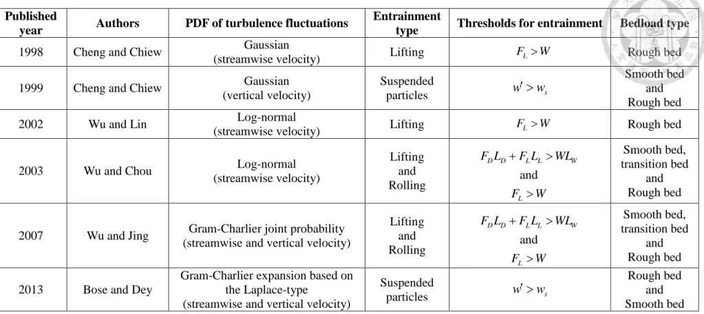
Bose and Dey (2013) raised the hypothesis that the sediment particles can be transported not only bedload motion by the velocity fluctuations in turbulent flows, but also as suspended load. Cheng and Chiew (1999) assumed that only the suspended particles are replaced with the bed load, and the wash load is egligible. It is said that the suspended particles at the top of the bed-load layer occur resuspension when the vertical
velocity fluctuations w of the turbulent flow exceeds the settling velocity ws of particles. Following this discussion, the vertical velocity fluctuations’ PDF, equation(2.4) obeyed the one-sided exponential-based Gram-Charlier series can be shown as
2
1 ˆ ˆ ˆ
( 0) 17 exp( )
16
( 0) 0
v
v
P w w w w
P w
(2.8)
Namely, they supposed that the instantaneous hydrodynamic force acting on a particle of the near bed velocity fluctuations is an important mechanism toward the sediment entrainment. In this assumption, the submerged weight of a particle is considered as a constant for a given particle size. Here, the probability of vertical velocity fluctuations contacts with the value of 2, and the value of 2 is related to the bed layer. Table 2.1 shows the comparison of previous studies. They also obtained the following expression for the relationship between 2 and bed layer property. For the bed layer is very thin, the bed is regarded as rough (Grass, 1971), it is
2 u*
. (2.9)
On the contrary, the bed is considered as smooth for thicker bed layer by Grass (1971), one can be written as
1.3
2 *
*
1 exp 0.093 u d u
. (2.10)
where u*, d and are shear velocity, particle diameter and kinematic viscosity of fluid, respectively.
Published
year Authors PDF of turbulence fluctuations Entrainment
type Thresholds for entrainment Bedload type
1998 Cheng and Chiew Gaussian
(streamwise velocity) Lifting FLW Rough bed
1999 Cheng and Chiew Gaussian
(vertical velocity)
Suspended
particles w ws
Smooth bed and
Rough bed
2002 Wu and Lin Log-normal
(streamwise velocity) Lifting FLW Rough bed
2003 Wu and Chou Log-normal
(streamwise velocity)
Lifting and
Rolling and
D D L L W
L
F L F L WL
F W
Smooth bed,
transition bed and
Rough bed
2007 Wu and Jing Gram-Charlier joint probability (streamwise and vertical velocity)
Lifting and
Rolling and
D D L L W
L
F L F L WL
F W
Smooth bed,
transition bed and
Rough bed 2013 Bose and Dey
Gram-Charlier expansion based on the Laplace-type
(streamwise and vertical velocity)
Suspended
particles w ws Rough bed
and Smooth bed
Table 2.1 Summary of previous study
2.3 Turbulent diffusion and dispersion
There are two categories of mixing process in a flow, diffusion and dispersion (Chien and Wan, 1999; Elder, 1958; Fisher et al, 1979; French, 1985). Diffusion can be used to describe the random scattering of particles, which is caused by molecular motion or eddy fluctuations, in the laminar flow field and the turbulent flow field, respectively. In contrast to diffusion, the variation of velocity distribution over the cross section leads to dispersion. In other words, dispersion is the scattering of particles associated with shear and transverse turbulent diffusion.
In this thesis, our focus is on the diffusion process. Following Roberts and Webster (2002) and Kirmse (1964), the velocity fluctuations of a turbulent flow have efficiently transport of momentum and heat. Comparing to molecular diffusion, the turbulent transport has more significant effect since the magnitude of eddy size is larger than molecular (i.e. turbulent energy is larger than molecular energy). The eddies are considered as continuous evaluation in time and its eddies range in size from Integral scales down to Batchelor scales. Pope (2000) indicated that even the flow with small length scale, the order of small length scale turbulence exceeds three or more orders of magnitude to the length scale of molecule. Figure 2.1 illustrates that the highest energy has the largest length scale, and also indicates that the Batchelor scale is much smaller than an order of magnitude than Kolmogorov scale.
The behavior of suspended particles is related to turbulent flow structure. The important concept in sediment theory is that the vertical concentration distribution is related to the ratio of turbulent sediment diffusion to momentum diffusion coefficient
(Cellino, 1998; Rouse, 1937; Tsujimoto, 2010). The ratio is a value which represents the difference between the diffusion of sediment particles and the diffusion of fluid particles (e.g. the molecule of water) in a flow. In 1937, Rouse obtained the turbulent sediment diffusion coefficient under the assumption of the log law for open channel turbulent flow. Without the supposition of log law profile, Absi et al. (2011) used the accurate analytical formulation for turbulent kinetic energy and eddy viscosity which calibrated by DNS data to calculate the coefficient of turbulent diffusion.
Figure 2.1 The classic turbulence energy spectrum versus to length scales for the open channel flow (Roberts and Webster, 2002).
2.4 Summary
In this chapter, different types of quantitative sediment transport methods are introduced (e.g. the Eulerian and the Lagrangian model). However, this study is focused on the Lagrangian model instead of the Eulerian model. Mechanisms such as sediment entrainment probability and diffusion coefficient are introduced in this section and more details will be mentioned in chapter 4. The aforementioned techniques will be applied to simulate sediment transport in chapter 5.
Chapter 3 Stochastic Theories
Equation Chapter (Next) Section 1
The specific objective in this thesis is to explore sediment transport in regular flow through an analysis of stochastic methods. Particles’ erratic behavior in fluid can be considered as stochastic, which may be caused by flow turbulence or particle interaction.
The Lagrangian model is used in this study in order to describe more details about particle motion. Moreover, different from the Eulerian model, the Langrangian model is more suitable and efficient to simulate the problem if the observer only concentrates on a particular region rather than the whole domain. Therefore, the particle tracking model based on the Lagrangian concept and the uncertainty characteristic is introduced. The abovementioned method is known as the stochastic diffusion process. Besides, there is another stochastic method called the stochastic jump diffusion process, which can be applied to condition of extreme flow events. This chapter introduces the simulation techniques of the stochastic theory such as the Markov process (or Markov chain) and the Wiener process (or Brownian motion) for particle tracking model. In addition, the numerical form for the stochastic differential process is also presented.
3.1 Markov Process
The Markov process is a stochastic process on a finite or countable number of possible values (Ross, 2007). In general, the possible value of the process is regarded as nonnegative integers (e.g.
0,1, 2,...
). The Markov chain in mathematical form can be given as
n 1 n , n 1 n 1,..., 1 1, 0 0
ijP X j X i X i X i X i P . (3.1) It indicates that in the process there is a sate i which will correspond to a fixed probability P . In other words, the property of Markov chain can be said that the future ij state is independent of the past states and will be influenced only by the present state. In this point, movement of a particle in a water system is assumed to be followed by the Markov process. For assumptions of the stationary process and Markovian property, there is a random walk theory of stochastic processes available to describe the state of sediment transport.
3.2 Brownian Motion
A pollen grain moved randomly in water is observed by Robert Brown in 1827, who named this phenomenon as Brownian motion. Regarding to molecular diffusion, a pollen grain has a stochastic trajectory. This phenomenon is based on the theory of random walk. Each particle moves left or right with the same probability 12, and obeys the well-known equation, Fick’s law. It can be noted that the motion of particle is independent because of the dynamic balance of retarding force and heat fluctuations. In spite of considering one-dimensional Fick’s law usually, the flux in an arbitrary direction is corresponding only to the concentration gradient in a specific direction, three-dimensional Fick’s law can be directly derived. For the concentration changing with time, the solution of unsteady state diffusion can be obtained as follows
1 2
( ) exp
4 4 c x,t x
Dt Dt
(3.2)
This distribution is the normal distribution with a zero mean and a variance of 2Dt. By means of the aforementioned concept, it can be easily assumed that the moving distance of a particle is the Gaussian distribution also with the same statistic properties (e.g. zero mean, standard divination, 2Dt).
Thanks to the contribution of Wiener and Levy, the mathematical expression of Brownian motion is also named the Wiener process or the Wiener-Levy process. The random walk theory is employed. Considering that the particle is released at origin, the position at time t can be shown as
1 [ ]
( ) ... t / t
X t x X X (3.3)
in which
t/t
is the largest integer less than or equal to t/t, and the Xi are assumed as independent values, obeying the same probability of moving left or right. It can be concluded that the Wiener process follows few conditions such asi) W(0) = 0 with probability 1.
ii) If 0 < s < t < T, then the random variable W W t( )W s( ) is the Gaussian distribution with mean and variance of 0 and (t - s) respectively, thus, the mathematical form can be written as ∆𝑊 = √𝑡 − 𝑠𝒩(0,1)
iii) The property of stationary independent increments. If 0 < s < t < u < v < T,
1 ( ) ( )
W W t W s
and W2 W t( )W s( )are independent.
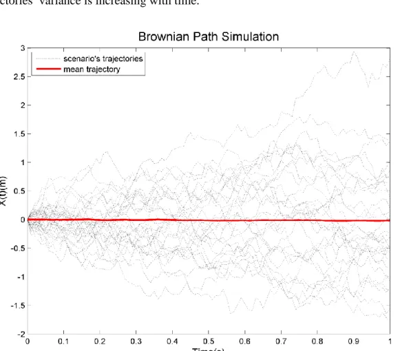
Figure 3.1 displays part of simple simulations of particle trajectory starting at
1 0
X and predicting the possible scenarios. In this example, time step t is given as
0.5 seconds, and the end of time is 1 second. The particles interaction is neglected, which means that particles have independently motions. We released 3000 particles at the origin, and the ensemble mean is calculated. The figure also shows that the trajectories’ variance is increasing with time.
Figure 3.1 Simulation of 3000 samples of the Wiener process
3.3 Stochastic Diffusion Process
The aim of differential equations is to describe the system of the time evolution.
For instance, the variable which is the function of time x t( ) within deterministic function is ordinary differential equations (ODE). In contrast, the system of the time
equation (SDE). The stochastic diffusion process is a type of stochastic differential equations, which can be expressed as follows.
( , ) ( , )
t
t t t
dX f X t g X t W
dt (3.4)
where Xt X t( ) is the realization of a stochastic process; f X t( t, ) is the drift term, which is presented as the deterministic part of the SDE and has the meaning of local trend; g X t( t, ) is the diffusion term, influencing the size of fluctuations in the SDE;
W is the Gaussian White noise process, which represents t dW dtt / . However, paths of the Wiener process are not differentiable. Depending on the choice of j (i.e. the integral manner of “left-hand” sum or “midpoint” sum), leading to the stochastic process to different kinds of stochastic calculus: Ito and Stratonovich; where jis in the time interval [ ,t tj j1] as shown in following sections.
Ito calculus
j tj
(3.5)
Stratonovich calculus
1
2
j j
j
t t
(3.6)
Using the symbol “o” in the Stratonovich concept to distinguish between SDEs interpreted in Ito and Stratonovich opinions, one obtain
( , ) ( , )
t
t t t
dX f X t g X t W
dt (3.7)
The stochastic integral between the Ito and Stratonovich calculus can be obtained respectively,
1
T
and
2 2
0
( ) d ( ) 1 ( ) (0)
2
T
W t W t W T W
(3.9)Since the Ito and Stratonovich interpretations do not converge to the identical form, using Ito’s formula to find a transformation from Ito to Stratonovich. The form equivalent to equation (3.4) can be given as
( , ) 1 ( , ) ( , ) ( , )
2
t
t t x t t t
dX f X t g X t g X t dt g X t dW dt
(3.10)
in which the modified drift term is called the noise-induced drift.
Although the Stratonovich interpretation is considered to be used within the physical property, the Ito interpretation is used in this study owing to the Markovian property (i.e. the future stat is only dependent on the present state).
3.4 Numerical Approximation for Stochastic Differential Equations
The Ito integral was introduced in the previous section. The numerical methods are introduced for solving equation(3.4) since most SDEs are unsolvable analytically.
Moreover, equation(3.4) can be rewritten in the differential form as
( , ) ( , )
t t t t
dX f X t dtg X t dW (3.11) Note that the initial position isX(0)X0 and that the time region is between 0 and T.
To apply the numerical methods such as the Euler-Maruyama (EM) method and Milstein method, first we need to discretize the interval. Assuming that the time
the numerical form of the EM method and Milstein method.
EM method
1 ( 1) ( 1) W( ) W( 1) , 1, 2,...,
j j j j j j
X X f X t g X j L (3.12)
Milstein method
1 1 1 1
2
1 1 1
( ) ( ) W( ) W( )
1 ( ) ( ) W( ) W( ) , 1, 2,..., 2
j j j j j j
j j j j
X X f X t g X
g X g X t j L
(3.13)
Both of these methods are the results of the Ito stochastic Taylor expansion by using the Taylor approximation. Here, the EM approximation in the Ito sense is a one-step approximation method, and converges with order 0.5 and 1 in the strong and weak sense, respectively. By adding all the stochastic increments, both of Milstein’s methods converge with order 1.
The strong and weak convergence definitions are as follows, and their convergence is equal to .
Strong convergence
n ( )
X X C t
(3.14)
in which C is a constant; is the expected value; Xn and X( ) are random variables, respectively; t is sufficiently small which fixs n t in the region of 0 to T.
Weak convergence
(3.15)
where the functions p in equation(3.15) obeys the conditions of smoothness and polynomial growth;
The above convergence definitions measure the rate of decay as t 0. As we can see, the convergence of strong measures the proportion of decay of “mean of error”.
In contrast, the convergence of weak is to measure the proportion of decay of “error of means”. Therefore, it can be concluded that weak convergence only takes into account the mean of solution. For instance, if the increment is √△ 𝑡𝒩(0,1) it can be replaced by any random variable which obeyed the same mean and variance such as sign function “sgn( )x ”, where x is a random number. There is a simple example to show the difference between the strong and weak convergence (Higham, 2001). The EM method is applied to the following equation in the linear form,
t t Xt t
dX X dW (3.16)
Equation(3.16) has an exact solution written as,
2 0
exp 1
t 2 t
X X tW (3.17)
The initial conditions and parameters in equation(3.16) in this example are shown in Table 3.1.
Parameter
X0 T dt
Value 1 2 0.1 1 2 , 2 , 2 , 2 , 29 8 7 6 5 Table 3.1 Some parameters and initial conditions in the example
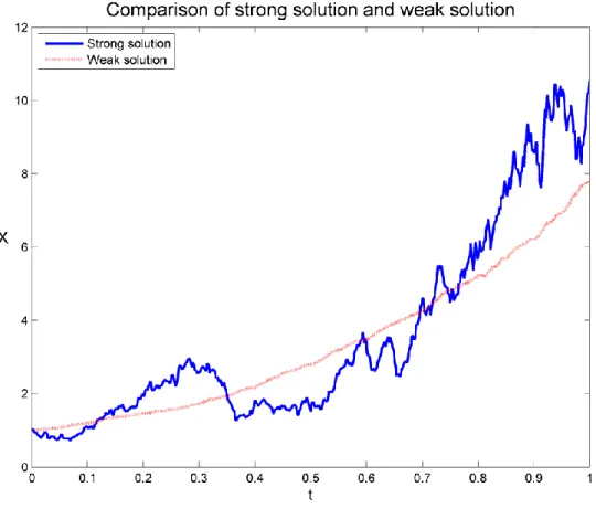
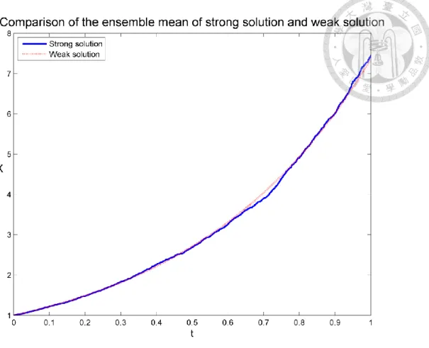
Figure 3.2 shows the comparison of one of scenarios with strong and weak solutions by using the time step 2-9. In this figure, it can be observed that the strong solution gives more information of paths than the weak solution. However, both of them have same statistic properties such as mean and variance. In Figure 3.3, the trajectories are almost the same if averaging the trajectories of both convergences. On the other hand, by using a least squares method, the convergence can be solved. In the strong solution, the convergence value is producing 0.5384 0.5 with a least squares value of 0.0266. The weak solution gives the convergence value 0.9858 1 with a least squares value 0.0508.
Figure 3.2 Comparing with Weak solution, strong solution emphases the information of path
Figure 3.3 Ensemble mean of strong solution and weak solution
3.5 Summary
The backgrounds of stochastic theories are introduced in this chapter. At first, the Markov theory is presented herein. The important mathematical form of the Wiener process (or Brownian motion) is also applied in the PTMs. With the aforementioned concepts, the stochastic differential equation can be constructed. Different types of mathematical interpretations such as the Ito scheme and Stratonovich scheme are appropriate in the respective problems. However, in this study, the Ito calculus is utilized since the hypothesis of Markovian property that the future state is only related to the present state. At the end of this chapter, different numerical schemes which enhance the numerical accuracy are also introduced. The EM method is ubiquitous and
Chapter 4 Development of Stochastic Particle Tracking Model of Suspended Sediment Transport
Equation Chapter (Next) Section 1
4.1 Introduction
Sediment particle movement in turbulent flow is difficult to describe exactly because of a large number of molecules in the flow and small particles’ collision. It takes longer to solve the equations of motion for all the molecules in the flow and for small particles. Moreover, the unknown of initial values of all the molecules in the flow and different motion of the small particles also puzzle the problem. To treat this problem in a simple way, the stochastic force is employed to describe the effect caused by molecules in flow and small particles’ collision (Risken, 1989). In other words, sediment particles or fluid particles in turbulent flow can be considered as a stochastic process. Based on the Markovian theory, the Fokker-Planck equation describes the conditional probability density for the fluid particle’s velocity and position as the evolution of time (Risken, 1989; Sawford and Borgas, 1994; Sharma and Patel,2010).
In general, the suspended sediment transport is simulated by the advection-diffusion equations by means of the deterministic solution of the Eulerian model. However, Dimou and Adams (1993) suggested that there are several reasons to use the Lagrangian model instead of the Eulerian model. Firstly, it is easier to represent sources in the Lagrangian model or the particle tracking model. The numerical problem
is more obvious to represent the region where most particles are located in the Lagrangian model rather than in the Eulerian model where all regions of the computational domain are considered equally. Thirdly, it is more effective to represent properties of the individual particles (e.g. particle diameter, settling velocity) in the Lagrangian model. To combine the characteristic of stochastic and the Lagrangian model, the Fokker-Planck equation which derived from Langevin equation (Gadiner, 1985) is used. Langevin equation describes the detail of individual particles in the Lagrangian framework instead of an assemblage of many particles. Since we cannot consider all the forces by molecules or particles collisions, by assuming these forces are random, the stochastic differential equation is constructed of deterministic forces.
Random force is introduced. Furthermore, the Fokker-Planck equation in the concept of the Markovian property, and the large number of particles at a very small time step corresponds to the advection-diffusion equation. However, some researchers have shown that it is not enough for considering a single particle model (Durbin, 1980;
Thomson, 1990; Borgas and Sawford, 1991; Borgas and Sawford, 1994). Durbin (1980) suggested that the autocorrelation of concentrations is needed for a complete stochastic theory of concentration fluctuations. The development of a particle tracking model is introduced in this chapter.
4.2 Model Assumptions
Assumptions regarding the particle tracking models are described as follows:
One-particle PTM
The SD-PTM is constructed based on the foundation of the random walk model.
The assumption is that particles are moved by the collision against adjacent fluid particles under a stochastic process, which is independent of the original position.
Random motion of sediment particles is described by the Wiener process. More details of the Wiener process are introduced in chapter 3.
Two-particle PTM
Different from one-particle PTM, this model tends to distinguish the effect by multiple scales of turbulence to describe more details of particle motion. The basic concept is that if their distance is close to zero, the motion of sediment particles is highly related to other particles caused by large scale turbulence. Particles can be separated by molecular diffusion if particles are in the immediate neighborhood. On the contrary, if their distance is large, sediment particles move independently. However, it is difficult to define how sediment particles move in response to various scales of eddies.
For simplification, it is hypothesized that the spatial correlation of sediment particles can be primarily attributed to large scales of eddies. As such, dependent Brownian motion can be used to simulate spatial correlation of particles constrained by large eddies. On the other hand, movement of sediment particles caused by molecular diffusion or smaller scales of turbulence is modeled by the independent Brownian motion.
4.3 Model Development
4.3.1 Stochastic Diffusion Model – One-Particle Particle Tracking Model
An aggregation of many particles is commonly employed instead of an individual particle. Fisher et al. (1979) applied an analysis of the concentration with no sources or sinks based on the deterministic continuity equation. Therefore, the equation with spatially varying coefficient in uniform flow can be written as
( s) x y z
change owing to advection change owing to diffusion
c c c c c c c
U V W w
t x y z x x y y z z
(4.1)
where c is concentration changing with time and space; U V W are the direction , , of x, y and z mean flow velocities, respectively, ws is particle settling velocity, and
, ,
x y z
are the sediment diffusion which represent all of the mechanisms causing mixing in the respective directions.
In 1985, Gardiner proposed that the random walk model which describes the position of each particle in Langevin framework, can be shown as
( , ) ( , ) t
deterministic forces
random forces
dx dB
A x t B x t
dt dt (4.2)
where A x t( , ) represents the deterministic forces, B x t( , ) is the random forces; and
t /
dB dt is a Gaussian White noise which represents the uncertainty nature of motion (Gardiner, 1985). Under the concept of Ito calculus, equation(4.2) can be rewritten as the form of a stochastic differential equation
( , ) ( , ) t
dx A x t dt B x t dB (4.3)