以雲解析模式探討中尺度對流渦漩對熱帶旋生之作用

(1)

國立臺灣大學理學院大氣科學研究所碩士論文

Graduate Institute of Atmospheric Sciences College of Science

National Taiwan University Master Thesis

以雲解析模式探討中尺度對流渦漩對熱帶旋生之作用 The Study on the Impact of Mesoscale Convective Vortices on Tropical Cyclogenesis using Cloud Resolving

Model

朱心宇 Hsin-Yu Chu

指導教授：吳健銘博士 Advisor: Chien-Ming Wu, Ph.D.

中華民國 108 年 8 月

August 2019

(2)

誌謝

光陰似箭，歲月匆匆，轉眼間已在為碩士論文的誌謝辭行文。這兩年學習了很多，

也成長了許多。進入研究所後，才發現自己之前所學多麼不足，不論是大氣科學專

業知識，還是Coding 等實務操作，兩者有許多要加強的部分。碩一下、碩二上修

習了健銘及維婷老師開的雲與環境專題及 ESM，在實務面上有許多精進，也感謝

指導教授健銘老師及維婷老師還有實驗室的學長姐們在每次 Meeting 時給予許多

寶貴的建議、經驗分享、有趣的 Talk 及教學。我是一個很喜歡自幹的人，也因為

這些經年累月累積的前人智慧，讓我能夠在碩二下半年間獨立完成實驗及論文。當然，在碩二下之前也有一段很長的徬徨及不安，在深夜時常常輾轉難眠及油然而生的自我質疑是否有做研究的資質。謝謝我大學時期認識的好麻吉，至誠、婉婷、學怡，偶爾一起去吃飯、Bar 喝酒放鬆抒發壓力。謝謝同為研究生的女朋友璟瑩，因為擁有共同目標所以假日常常都泡在咖啡店做實驗，寫論文，能互相激勵、抱怨並體諒為甚麼約會時常那麼無趣，這段時間沒有妳我真的不知道該怎麼走下去。

最後，我要感謝我的父母親，這一年對我們家來說真的是轉變很大的一年，連續有兩位至親生病離開，但照顧至親，傷痛之餘還是持續支持我，讓我能無憂無慮完成學業。謝謝你們從小就尊重我的夢想及志向，在台灣就業導向為主選科系，別人不理解為甚麼我要選擇大氣科學這條路時還是給予我莫大的鼓勵。

大氣科學之博大精深，期許自己在未來還能持之以恆，繼續奉獻微薄之力。

朱心宇謹致

2019 年 8 月

于國立臺灣大學大氣科學研究所

(3)

中文摘要

此研究中，我們於三維雲解析向量渦度模式中(VVM)植入六組最大風速位於不同高度的雷坎渦旋 (Rankine Vortex)，分別代表位在不同高度的理想化中尺度對流渦漩 (Mesoscale Convective Vortex, MCV)，藉此評估不同 MCV 造成的垂直擾動位溫結構對旋生過程的影響。前人之研究中指出，由於平衡熱力的結果，在潛在位渦 (PV)最大值高度以上，會有正位溫距平，而在其下會有負位溫距平，造成垂直位溫結構趨於穩定。這個距平容易激發垂直質量通量(MF)最大值在中低對流層之

“Bottom-Heavy” 對流系統。此種對流結構會增強底部水氣輻合，增加整體氣柱的飽和比(SF)，或者透過海表焓通量作用，激發更多對流。而底部輻合也會透過渦度垂直拉伸項造成底層渦旋加強。

我們發現初始雷坎渦旋最大風速(𝑣𝑚𝑎𝑥)高度位在 4.5 公里的實驗最早發生，領

先其他組實驗7 小時以上。由此可知，MCV 最大風速高度位在 4.5 公里為最有利

旋生之高度。另外，當渦旋初始最大風速高度在地表或7.5 公里以上，模式積分 144

小時之後仍不會發生旋生，顯示MCV 造成的熱力調整可能影響到旋生的過程。由

實驗發生旋生與否，我們能進一步將實驗分成發展組(DS)跟不發展(NDS)組。為了進一步分析和濕熵及濕熵的時序變化，我們將高層及低層大氣的飽和濕熵差值定義穩定度指數(SI)，其數值越小代表穩定度越大。DS 組的 SI 在旋生前 48 小時開始即有系統性的減少，而在旋生前 0-12 小時區間 DS 的 SI 中位數比 NDS 低 5

JK^-1kg^-1左右。同時DS 的氣柱飽和比 NDS 的氣柱飽和比高，而且隨著時間接近旋

生，DS 的 SF 同樣的會有系統性的增加。SI 與 SF 之聯合分布的結果，SI 大致上

與SF 呈現反比，顯示熱力環境的穩定伴隨氣柱的飽和。

根據前人雲解析模擬的結果，在環境處於高氣柱飽和比時，較容易產生極端降水及大型組織性對流系統。於旋生前環境中具有高渦度量值的對流系統，即所謂的渦度熱塔(Vortical Hot Tower, VHT)，而 VHT 的增加及合併在旋生時增加環境渦度及加熱，扮演重要的角色。本研究透過六向連通元件標記法，先將三維空間中的雲

元件標記出來，再將雲厚大於10 公里的雲元件定義為 VHT。我們發現，DS 在旋

生前 36 小時前，靠近渦旋中心 100×100 km²之區域出現體積大於10⁴km³之渦度

熱塔之機率密度即超過 NDS。最後透過定量分析垂直質量通量在低 SI 與高 SI 之

機率分布，發現在低 SI 的環境中較容易產生 Bottom-Heavy 的對流。對流更有效

率的集結及產生Bottom-Heavy 的垂直質量通量，有助於初始渦旋透過加熱及渦度

拉伸等機制，讓低層渦度增強。

關鍵字: 熱帶旋生、中尺度對流渦旋、垂直質量通量、氣柱飽和比、渦度熱塔

(4)

Abstract

In this study, Rankine vortices that represent idealized Mesoscale Convective Vortex (MCV) with maximum wind speeds at different levels embedded in a quiescent tropical environment are studied using Vector Vorticity Model (VVM), a three-dimensional, cloud resolving model. We aim to evaluate how different extent of the potential temperature profile modulates the evolution of the initial vortex. Under balanced thermodynamics, positive (negative) potential temperature anomaly will be present above (below) maximum level of potential vorticity. If such profile is optimally placed, the corresponding stabilization is theorized to enhance “bottom heavy” mass flux profile, inducing convergence at lower level, further promoting column saturation and precipitation, contributing to the spin-up of the low-level vortex.

The experiment with a Rankine vortex where maximum wind (𝑣𝑚𝑎𝑥) located at z = 4.5 km, is the earliest to undergo cyclogenesis, leading other runs by approximately 7 hours or more. The vortex with 𝑣𝑚𝑎𝑥 at sea level or above 7.5km, does not develop after 144 hours. The time required to reach cyclogenesis is proportional to the difference between the level in which 𝑣𝑚𝑎𝑥 is located below or above 4.5 km, where z = 4.5 km seems to be the optimal height to promote genesis. Based on cyclogenesis occurs in 144 hours or not, we can categorize them into developing sets (DS) and non-developing sets (NDS). To analyze the stabilization of thermodynamic environment, we define stability index (SI) based on the difference of saturated moist entropy (s*) between upper and lower troposphere. Smaller (larger) values of SI indicates higher (lower) environmental stability. 48 hours prior to the genesis, the SI of DS systematically decreases, and during the period 0-12 hours prior to the genesis, the median SI of DS is around 5JK^-1kg^-1lower than that of NDS. The saturation fraction (SF) in DS also shows a systematic increase prior genesis. Joint-PDF of SI and SF confirms the fact that SF is inversely proportional to SI, demonstrating stabilization is accompanied by column saturation.

In an environment with higher saturation fraction is more likely to produce large, organized convection. Convective structures that are highly rotational in cyclogenetic environments are phrased as “Vortical Hot Towers (VHTs)” and the increase in number and merger of VHTs plays a notable role as a source of vorticity convergence and heating during genesis. Here we identify the size, height and other characteristics of clouds by connecting cloud grids together as cloud objects using a six-connected segmentation algorithm. After cloud objects are labeled, VHTs are then filtered using cloud thickness exceeding 10 km as the criteria. We then compare the size distribution of these VHTs between the DS and NDS. In the DS, probability density of large VHTs with volumes over 10⁴ km³ within a 100×100 km² square box around the vortex center steadily

(5)

overpasses NDS, which is a sign of aggregation and upscale growth 24-36 hours prior to the genesis. Finally, we show that the generation of “bottom-heavy” mass flux profile is more likely in low SI environments by comparing the probability distribution of a bottom- heavy index in low SI and high SI environments. The tendency to generate large VHTs and bottom-heavy mass flux profiles, promotes processes such as organized heating and stretching, which intensifies the incipient vortex.

Keywords: Tropical Cyclogenesis, Mesoscale Convective Vortex, Vertical Mass Flux , Saturation Fraction, Vortical Hot Tower

(6)

List of Figures

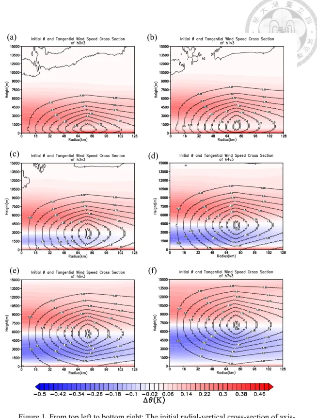
Figure 1. From top left to bottom right: The initial radial-vertical cross-section of axis-symmetric perturbed 𝜃 (shaded) and wind speed (contoured) of (a) h0v3 (b) h1v3 (c) h3v3 (d) h4v3 (e) h6v3 and (f) h7v3. Perturbed 𝜃 is defined as the difference of 𝜃 at the point and domain average.

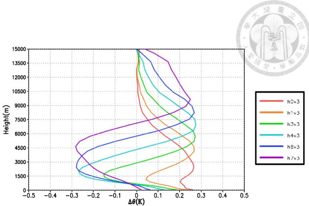
Abscissa is the distance between the vortex center. ... 11 Figure 2. Vertical profile of the perturbed potential temperature at the center

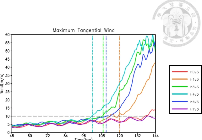
of the vortex center caused by the initial MCV. The perturbed potential temperature is calculated as the difference between the 𝜃 at the vortex center and the domain averaged 𝜃 ... 12 Figure 3. Time series plot of azimuthal averaged maximum 10-meter height

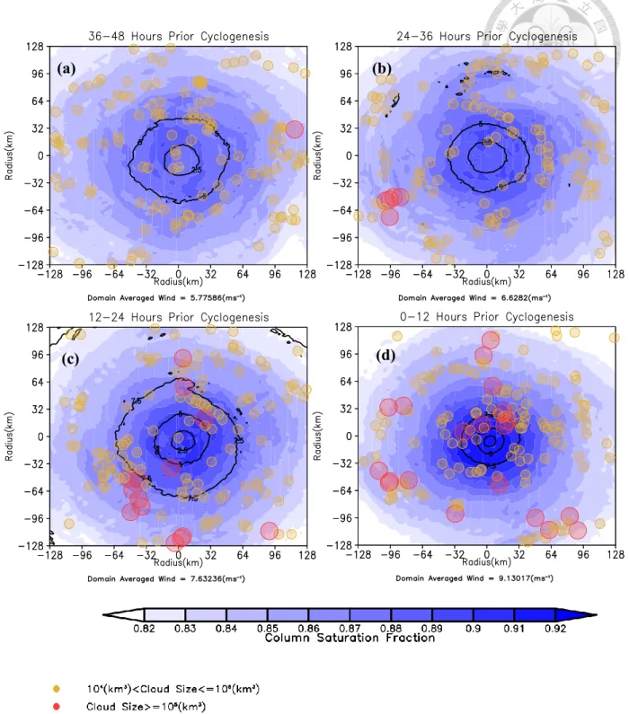
tangential wind of different sensitivity experiments. Vertical lines denote tg. and the horizontal lines denote 10 ms^-1. ... 17 Figure 4. Evolution of averaged composite saturation fraction, shown in

shaded, geometric center and the size of VHT objects of h4v3 and h3v3 at the time period (a) 36-48 Hours (b) 24-36 (c) 12-24 (d) 0-12 hours prior genesis. The wind speed is contoured from 2.5-7.5 ms^-1, at an interval of every 2.5 ms^-1. ... 21 Figure 5. Same as Figure 4, but for NDS. ... 22 Figure 6. Hovmöller diagram of difference in azimuthally averaged saturation

fraction between DS and NDS. Blue (red) denotes positive (negative) anomaly of DS relative to NDS. Positive anomaly that exceeds 0.05 is marked with contours. ... 23 Figure 7. Evolution of averaged s* (top) and s (bottom) in a 100×100 km² box

around the vortex center, indicated at the time interval. The solid lines are the DS and dashed line are the NDS. ... 26 Figure 8. Difference between averaged s (red) and s* (blue) in a 100×100 km²

box of DS and NDS (∆𝑠 = sds - snds) 24-36 hours (left) and 0-12 hours (right) prior to cyclogenesis ... 27 Figure 9. Hovmöller diagram of sds* - snds*, the difference of saturated moist

entropy between DS and NDS, abscissa denotes height in meters ... 27 Figure 10. Box plot of averaged SI at the interval stated in the abscissa, prior

genesis, in a 100×100 km² box around the vortex center for NDS (top) and DS (bottom). The black bar denotes the extent of the maxima and minima. The blue box is the range between first quartile and third

(8)

quartile. The red line denotes the median. The red cross denotes the outliers. ... 29 Figure 11. Scatter plot of average precipitation in a 48 hours period prior to

genesis of top 1% (open circle) and all samples (plus sign) in a 100×100 km² box around the vortex center box, binned by saturation fraction of 0.02. ... 33 Figure 12. Box plot of area averaged SF sampled at the interval stated in the

abscissa, prior genesis, in a 100×100 km² box around the vortex center for NDS (top) and DS (bottom) ... 34 Figure 13. Log10-scale joint probability distribution of column saturation

fraction versus stability index of (a) DS and (b) NDS. Sample are taken from 0-48 hours prior genesis in a 100×100 km² box around the vortex center. The average precipitation of each grid on the joint-probability space are contoured. ... 38 Figure 14. The difference of log10 PDF between DS and NDS. Regime with

difference in P>10^0.3are marked with contour. ... 39 Figure 15. Scatter plot between SF and mean SI, binned by 0.01 interval,

sampled during (a) 0-12 hours and (b)24-36 hours prior cyclogenesis in a 100×100 km² box around the vortex center. The dashed line denotes the averaged stability index for DS (red) and NDS (green). ... 42 Figure 16. Azimuthally averaged [∇ ⋅ 𝜌𝑣𝑠] of DS (red) and NDS (green),

averaged during 0-12 hours period prior genesis. ... 43 Figure 17. The (a) Domain Wide Cloud Object (b) Cloud Object Count in a

100×100 km² box around the vortex center. The data is low pass filtered to exclude half-day diurnal variations. ... 45 Figure 18. Same as Figure 17, but for the counts of VHTs ... 46 Figure 19. Histogram of VHT Size in DS (D, in blue), and NDS (ND, in red),

during (a) 36-48 hours (b) 24-36 hours (c) 12-24 hours (d) 0-12 hours prior genesis in a 100×100 km² box around the vortex center ... 47 Figure 20. Same as Figure 19, but sampled in the entire domain... 47 Figure 21. The error bar plot of VHT size versus area averaged SI in a

100×100 km² box around the vortex center. The extent of error bar is the maximum/minimum size of VHTs in each bin. The sample is taken in the period 0~48 hours prior genesis, in the same area, and size of VHTs are binned by 1.0 unit of stability index. ... 48 Figure 22. Same as Figure 21, but for NDS. ... 48 Figure 23. 3D Snapshot of VHT object (in white), iso-surface of vertical

vorticity with 𝜁 + 𝑓 > 1.5×10³ s^-1 and the contour of vorticity with

(9)

values greater than 5.0 ×10³ s^-1 (in green) at 2000 m of Experiment h4v3 at (a) 48 hours (b) 36 hours (c) 24 hours and (d) 12 hours prior genesis ... 54 Figure 24. Averaged vertical mass flux in a 100×100km² box placed at the

vortex center of (a) DS and (b) NDS averaged in the given period ... 55 Figure 25. Averaged convective vertical mass flux in a 100×100 km² box

placed at the vortex center of (a) DS and (b) NDS averaged in the given period ... 56 Figure 26. The evolution of composite VHT fraction of DS (solid line) and

NDS (dashed line) in a 100×100 km² box around the vortex center in the indicated period. ... 57 Figure 27. The conceptual diagram of modified vertical mass flux Mz (in

green), kernel K (in red) and integrand K(z)Mz (in blue) of (a) Bottom Heavy Case (b) Top Heavy Case ... 58 Figure 28. The probability of bottom-heaviness index (BI) sampled (1)

Bottom 25% of SI (in red) (2) Top 25% of SI (in green) for DS (solid line) and NDS (dashed line) ... 59 Figure 29. Flow chart of an updated cyclogenesis framework combining the

VHT paradigm and the role of stabilization caused by MCV. ... 63

(10)

List of Tables

Table 1. The level of maximum velocity, Zmax, maximum tangential wind, Vmax, radius of maximum wind, Rmax and e-folding scale, A, for the implanted Rankine vortex of the sensitivity experiments ... 9 Table 2. Cyclogenesis time (tg), post-genesis time (tpg) and the time it takes to

reach genesis (tpg- tg)... 18 Table 3. Quantiles of stability index averaged over 100×100 km² box around

the vortex center sampled in the given period. ... 30 Table 4. Quantiles of saturation fraction averaged over 100×100 km² box

around the vortex center sampled in the given period. ... 35

(11)

Chapter I. Introduction

Tropical cyclogenesis, the process of a tropical cloud cluster transforming into a

quasi-stable, long-lasting mesoscale vortex, is a multiscale and finite amplitude process

(Emanuel, 1989). During the last few decades, different theories were proposed to

explain the processes involved in tropical cyclogenesis, which can be divided into two

main school of thoughts. “Top-down” development proposes that low-level cyclone

develops by the down-transport and merger of vorticity that source from mesoscale

convective vortices (MCV, Bister & Emanuel, 1997). The “bottom-up” development

theory (Hendricks et al., 2004; Montgomery et al., 2006) proposed that rotating deep

convection, which they called vortical hot towers (VHT), are main coherent structure

embedded in the MCV. The existence of MCV creates vertical wind shear, hence

horizontal vorticity components. These VHT forms by tilting of horizontal vorticity

through updrafts, and are able to spin up the vortex through multiple diabatic merger

events. The merger of VHTs have two major contributions to vortex spin up: (1) the

contribution in stretching term in vertical vorticity equation through intense helical

motions and (2) diabatic merger collectively heating up the lower troposphere near the

center of the incipient vortex, creating a secondary circulation due to radial gradient of

diabatic heating.

(12)

The collective effects of diabatic heating from the deep convection near the regions of

high inertial stability induces a toroidal secondary circulation, which could be explained

from the RHS in the balanced Sawyer-Eliassen Equation on a cylindrical coordinate

(Schubert & Hack, 1982):

𝜕

𝜕𝑟

(𝐴

^{𝜕(𝑟𝜓)}

𝑟𝜕𝑟

+ 𝐵

^𝜕(𝜓)

𝜕𝑧

) +

^𝜕

𝜕𝑧

(𝐵

^{𝜕(𝑟𝜓)}

𝑟𝜕𝑟

+ 𝐶

^𝜕(𝜓)

𝜕𝑧

) =

^𝑔

𝜃₀

𝜕𝑄

𝜕𝑟

(Eq. 1)

A, B and C represents static stability, baroclinity and inertial stability respectively. g is

gravitational acceleration and 𝜃₀ is a reference value of potential temperature. 𝑄 is the

diabatic heating rate and 𝜓 is the mass stream-function on (r,z) plane. The amplification

in this secondary circulation induces increased low-level inflow that precedes wind

induced surface heat exchange (WISHE, Rotunno & Emanuel, 1987) to spin up the

incipient vortex.

Although the exact framework leading to genesis remains uncertain, column

saturation is commonly observed to precede tropical cyclogenesis. According to many

studies (Dunkerton et al., 2009; Nolan, 2007; Wang, 2018), it is evident that the region

near the center of incipient disturbance will reach and remain near column saturation

prior to the cyclogenesis. The sustained moisturization will “lock” the development of

convection in the inner region close to the vortex center, preventing gravity waves from

dissipating energy to the quiescent environment and continue to moisturize the

environment through diabatic heating.

(13)

Recent advances in high resolution cloud modeling opened an opportunity to marry

these two school of thoughts. Raymond and Sessions (2007) uses a two-dimensional

cloud model to study the evolution of convection in different magnitudes of stabilization

of thermodynamic profile through adding different magnitudes of potential temperature

perturbation at 3000m and 10000m into a background environment under radiative-

convective equilibrium (RCE). Their result revealed that a more stable potential

temperature profile will lead to a convective vertical mass flux that is concentrated in the

lower-middle troposphere, which is “bottom-heavy”, as opposed to the “top-heavy”

convective vertical mass flux profile in a environment under RCE. This allows vorticity

convergence in lower troposphere and ventilation of high entropy air into the

atmospheric column through mass convergence and detraining the lower entropy air in

the mid-troposphere. In addition to numerical studies, observational studies

(Gjorgjievska & Raymond, 2014; Raymond et al., 2011) using data from THORPEX

Pacific Asian Regional Campaign/Tropical Cyclone Structure Experiments

(TPARC/TCS-08) also showed an evolution of convection from “top-heavy” to “bottom-

heavy” prior the genesis of tropical storm Nuri, and showed that the “bottom-heaviness”

of convection in the environment is related to the stabilization of environment.

Additionally, they found that the stabilization of environment is inversely related to the

saturation fraction, and proportional to the vorticity at mid-levels.

(14)

Based on these results, Raymond et al. (2014) proposed a framework to explain how

the existence of a mid-level vortex can provide a favorable environment for the

intensification of a surface vortex. First they discussed that the early misconception that

“direct down (up) transport” of mid-level vorticity or any rotating systems on different

scale appearing in both “top-down” and “bottom-up” theories to amplify the surface

vortex is not possible, postulated by Kelvin’s Circulation Theorem. Alternatively, the

role of MCVs is the supply of a stabilized saturated entropy (s*) environment due to

thermal wind balance, and the stabilized environment can promote “bottom-heavy”

convection, inducing sustained feedback of environment moisturizing, which creates a

positive feedback through stretching to increase low-level vorticity. This conclusion is

intriguing due to the attempt to marry the “top-down” meso-𝛽 environment triggering a

“bottom-up” upscale cascade of vorticity by convective scale aggregations.

This study aims to supplement the framework of Raymond and Sessions (2007).

First, we want to test if their hypothesis from two-dimensional configuration and

horizontally homogeneous potential temperature perturbation is also valid in a three-

dimensional environment. We use a different approach, implanting idealized,

axisymmetric vortices in a three-dimensional cloud resolving model and let the

thermodynamic environment adjusts to the vortex to achieve the stabilization analogous

to their initial condition. Second, since heating/cooling of the troposphere can produce

(15)

different MCV structures, we want to test if different vertical profiles of initial MCV

influence the evolution of the low-level vortex. Chapter 2 describes model and the

experiment setup. Chapter 3 analyzes the evolution of environment in these experiments.

Chapter 4 presents the evolution of convection under different environments.

Concluding remarks and future work are discussed in Chapter 5.

(16)

Chapter II. Methodology 2.1 Vector vorticity model

The core of this study is to analyze how the intricate structural transition of moist

convection in a pre-existing mid-level vorticity aids cyclogenesis. To reach our purpose,

we use a high resolution, cloud resolving model, Vector Vorticity Model (Jung &

Arakawa, 2008) to implement our experiment. VVM uses 3-dimensional anelastic

vorticity equation as the prognostic equation of horizontal dynamics instead of

momentum equation. One of the advantages of using vorticity equation instead of

momentum equation is that the pressure gradient term is removed in the material

derivative equation, eliminating the need to predict pressure. VVM was used to study

the behavior of cloud systems in a wide range of spatial-temporal spectrum and applied

to improve current cloud parameterization methods. In climate spectrum, VVM is used

to study spontaneous aggregation under varying environments such as rotating and non-

rotating radiative-convective equilibrium (Tsai & Wu, 2017; 吳蔚琳, 2017; 陳彥婷,

2018) and during suppressed phase of Madden-Julian Oscillation (MJO, 陳逸昌, 2016).

In meso-beta and cloud scale, VVM is previously used to study the interaction of meso-

beta environment, clouds and topography. For example, critical transition of maritime

stratocumulus (Tsai & Wu, 2016), the study of land-atmosphere interaction in the

evolution of maritime convection ( 陳柏言 , 2018), improved representation of

(17)

convection over topography using immersed boundary method (Chien & Wu, 2016; Wu

& Arakawa, 2011), evolution of afternoon thunderstorms in Taipei Basin (Kuo & Wu,

2019) and the formation of upslope fog in Montane cloud forests (謝旻耕, 2019). In

improving cloud parameterization, VVM is used to establish a unified parameterization

scheme of moist convection (Arakawa & Wu, 2013; 郭威鎮, 2017) and improvements

in representing sub-grid scale convective process using a machine learning method

called 3D convolutional neural network (3D-CNN, 鄒適文, 2019).

(18)

2.2 Initial condition and model setup

MCVs originate from the stratiform regions in tropical mesoscale convective

complex (MCC, Houze Jr., 2004). These MCVs are theorized to generate by the broad

evaporative cooling and downdraft heating in these regions and promotes low-level

cyclogenesis through various mechanisms. Previous research such as Nolan (2007) and

Montgomery et al. (2006) uses idealize a Rankine vortex, representing a MCV with

potential vorticity maxima at 4000 m to simulate the related mechanisms. However, as

differential heating caused by subsidence warming in stratiform region and evaporative

cooling can generate different baroclinic modes which places maximum positive and

negative anomaly of potential temperature at different levels in realistic atmosphere, to

study how tropical cyclogenesis are effected by such difference, an idealized axis-

symmetric Rankine vortex are placed with maximum wind speed at different vertical

level, following the below equation:

𝑉(𝑟, 𝑧) =

{

𝑣(𝑧) ^𝑟

𝑅_𝑚𝑎𝑥 (𝑖𝑓 𝑟 < 𝑅_𝑚𝑎𝑥)

𝑣(𝑧)^𝑅^𝑚𝑎𝑥

𝑟 (𝑖𝑓 𝑅𝑚𝑎𝑥 ≤ 𝑟 < 3𝑅𝑚𝑎𝑥 ) 𝑀𝐴𝑋 [^𝑣(𝑧)

5 (1 −^𝑟−3𝑅^𝑚𝑎𝑥

𝑅_𝑚𝑎𝑥 ) , 0] (𝑖𝑓 𝑅𝑚𝑎𝑥 ≤ 𝑟 < 3𝑅𝑚𝑎𝑥 )

(Eq. 2)

Where 𝑣(𝑧) = 𝑣_𝑚𝑎𝑥𝑒𝑥𝑝 (−^(𝑧−𝑍^𝑚𝑎𝑥⁾²

𝐴 )

All the perturbations are placed relative to the center of the domain. 𝑅_𝑚𝑎𝑥 is the radius

at which horizontal wind is maximum, 𝑍_𝑚𝑎𝑥 is the level at which the horizontal wind

is maximum, and 𝐴 controls the vertical e-folding scale. We include six sets of

(19)

sensitivity experiments by increasing the value of 𝑍_𝑚𝑎𝑥 at a interval of 1500 m, shown

in the Table 1.

Experiment

Name 𝑍_𝑚𝑎𝑥(m) 𝑣_𝑚𝑎𝑥(𝑚𝑠⁻¹) 𝑅_𝑚𝑎𝑥(km) 𝐴

h0v3 0 3 75 2.0 × 10⁷

h1v3 1500

Same As Above

h3v3 3000

h4v3 4500

h6v3 6000

h7v3 7500

Table 1. The level of maximum velocity, Zmax, maximum tangential wind, Vmax, radius of maximum wind, Rmax and e-folding scale, A, for the implanted Rankine vortex of the sensitivity experiments

The GARP Atlantic Tropical Experiment (GATE) average sounding is used as the

initial water vapor mixing ratio and potential temperature profile. The cloud microphysics

used in this experiment is a three-phase microphysical scheme (Krueger et al., 1995),

which water vapor(𝑞_𝑣), cloud water (𝑞_𝑐), rain (𝑞_𝑟), graupel (𝑞_𝑔), cloud ice (𝑞_𝑖) and snow

(𝑞_𝑠) are prognostic variables. The Coriolis parameter are set to 1.9 × 10⁻⁵ s⁻¹, the

approximate value at 25^°N. Radiative transfer is parameterized with -2 K Day^-1 cooling

in the troposphere. The sea surface temperature (SST) are set to a constant value of 303

K, an idealized climatological value of Western Pacific Ocean Warm Pool. Random

(20)

perturbations are applied at 20 minutes after model integration, creating some weak

temperature gradient allowing development of convection.

The radial-height profile of azimuthal averaged tangential wind speed and perturbed

potential temperature, defined as the local potential temperature subtract the domain

average, three hours after model initialization, is shown in Figure 1. Evidently, after an

initial adjustment process, with Zmax of the initial vortex at different level, different

perturbed 𝜃 profiles is generated. There is positive potential temperature anomaly in

the mid-lower troposphere for experiment that Zmax is located lower in the troposphere

(h0v3, h1v3), while others creating a negative anomaly in the mid-lower troposphere.

The depth of negative anomaly depends on the height of Zmax. Figure 2 shows the

amplitude of perturbed 𝜃 at the center of the initial vortex.

(21)

(a) (b)

(c) (d)

(e) (f)

Figure 1. From top left to bottom right: The initial radial-vertical cross-section of axis- symmetric perturbed 𝜃 (shaded) and wind speed (contoured) of (a) h0v3 (b) h1v3 (c) h3v3 (d)

h4v3 (e) h6v3 and (f) h7v3. Perturbed 𝜃 is defined as the difference of 𝜃 at the point and domain average. Abscissa is the distance between the vortex center.

(22)

Figure 2. Vertical profile of the perturbed potential temperature at the center of the vortex center caused by the initial MCV. The perturbed potential temperature is calculated as the difference between the 𝜃 at the vortex center and the domain averaged 𝜃

(23)

2.3 Diagnostic packages

2.3.1 Vortex tracking

Low Level Circulation Center (LLCC) of the vortex is defined as the local maxima

of horizontal stream-function at z=1.5km, defined as (^𝜕²

𝜕𝑥²+ ^𝜕²

𝜕𝑦²)𝜓 = (𝜁 + 𝑓). We use successive over-relaxation (SOR) as our numerical method for the discrete Poisson

solver. The terminating condition is set as the relative difference between the stream-

function solved in the previous iteration and the current iteration satisfies:

𝑒𝑟𝑟 ≡ |^𝜓^𝑛^−𝜓^𝑛−1

𝜓𝑛 | < 10⁻⁴% (Eq. 3) to insure the convergence in solution of the stream-function.

2.3.2 Cloud Object Labeling and VHT Filtering

To analyze the effect of an existing MCV to the cloud structure, we first define an

individual cloud grid as a grid point in model domain that satisfies the criteria 𝑞_𝑖+ 𝑞_𝑐 ≥

5 × 10⁻⁵ kg kg⁻¹, and then implement six-way connected segmentation method (陳逸昌, 2016) to group connected grid points to form a cloud object. We then separate cloud

objects, with the criteria of maximum in cloud vertical velocity, 𝑤 ≥ 0.5 m s⁻¹ as

convective and otherwise non-convective. Convective cloud objects can then be

separated into deep convection with cloud base under 2 km and cloud top over 12 km

and other convective clouds.

(24)

To study the occurrence of convection in the inner region of a vortex, we need a

method to determine if the cloud object lies inside the inner region or outside. Clouds

are three-dimensional structure that area and position that varies with height, so we think

that it is unfair to evaluate the position of cloud only based its position at certain level.

Consequentially, we use the geometric centroid of the cloud object, defined as:

(𝑥 ̅̅̅, 𝑦

_𝑐

̅ ) =

_𝑐 ¹

𝑁

(∑

^𝑖=𝑁_𝑖=1

𝑥

_𝑖

, ∑

^𝑖=𝑁_𝑖=1

𝑦

_𝑖

)

(Eq. 4) Where index i denotes a grid point of the cloud object.

2.3.3 Moist Thermodynamic Variables

In later chapters, “stabilization of environment” specifically means the reduction in

difference of saturated moist entropy between two vertical levels. Defining moist entropy

using a more detailed version derived from Carrillo and Raymond (2005), which

incorporates freezing process into the calculation of moist entropy:

𝑠 = (𝐶_𝑝𝑑+ 𝐶_𝑝𝑣𝑞_𝑣+ 𝐶_𝑙𝑞_𝑙+ 𝐶_𝑖𝑞_𝑖) ln (^𝑇

𝑇_𝑟) − 𝑅_𝑑ln (^𝑃^𝑑

𝑃_𝑟) − (𝑅_𝑣𝑞_𝑣) ln (^𝑃^𝑣

𝑃_𝑡𝑝) + (^𝐿^𝑐^𝑞^𝑣^−𝐿^𝑓^𝑞^𝑖

𝑇_𝑟 ) (Eq. 5)

Here, Cpd = 1005 J K^-1 kg^-1, Cpv = 1850 J K^-1 kg^-1, Cl =4218 J K^-1 kg^-1, Ci = 1959 J K^-1

kg^-1denotes the heat capacity of dry air, water vapor at constant pressure, liquid water

and ice. 𝑞_𝑣, 𝑞_𝑙, 𝑞_𝑖 denote the mixing ratio of water vapor, liquid water and ice (kg kg^-1).

𝑇 the temperature (K). 𝑇_𝑟 = 273.15 K, the freezing point for water. 𝑅_𝑑 = 287.05 J K^-

1 kg^-1, 𝑅_𝑣 = 461.5 J K^-1 kg^-1 is the gas constant for dry air and water vapor. 𝑃_𝑑, 𝑃_𝑣 is

the partial pressure for dry air and water vapor. 𝑃_𝑡𝑝 = 6.1078 hPa , the triple point

(25)

pressure for water. 𝑃_𝑟 = 1000hPa, the reference pressure. 𝐿_𝑐 = 2.5008 × 10⁶ J kg^-1,

𝐿_𝑓 = 3.337 × 10⁵ J kg^-1,the latent heat of condensation and freezing. Saturated moist

entropy (s*), is calculated by replacing 𝑞_𝑣 with 𝑞_𝑣^∗ , the saturated mixing ratio, and

letting 𝑞_𝑙 = 𝑞_𝑖 = 0 . 𝑞_𝑣^∗ (𝑇, 𝑧) is derived using Clausius-Clapeyron equation from the

temperature of a specific grid point.

Since VVM does not explicitly output temperature but dry potential temperature (𝜃) as

prognostic variable. For the requirement of calculating moist entropy, we define

temperature (K) as:

𝑇(𝑥, 𝑦, 𝑧, 𝑡) = [𝜃(𝑥, 𝑦, 𝑧, 𝑡) (^𝜌𝑅^𝑑

𝑃_𝑟)

𝑅𝑑 𝑐𝑝]

1 1−𝑅𝑑

𝑐𝑝 (Eq. 6)

To calculate the relation between column saturation, stability index and precipitation, we

define saturated fraction as:

𝑆𝐹 ≡

^{∫ 𝜌(𝑠−𝑠}^𝑑^)𝑑𝑧

ℎ 0

∫ 𝜌(𝑠₀^ℎ ^∗−𝑠_𝑑)𝑑𝑧 (Eq. 7)

Where 𝑠, 𝑠^∗, 𝑠_𝑑 each corresponds to the moist entropy, saturated entropy and dry

entropy. The integrand is integrated from sea level to model level top.

(26)

Chapter III. Analysis of large scale environments

3.1 Maximum tangential wind and genesis time

The evolution of azimuthal averaged maximum tangential wind speed at sea level

(Vθmax) is shown in Figure 3. Initially, the Vθmax of all the experiments remains relatively

weak at 5-10 ms^-1 for approximately 100 hours. After 100 hours, h1v3, h3v3, h4v3 and

h6v3 experienced a sudden “trigger” in intensification, with h3v3, h4v3, and h6v3

intensifying from 10ms^-1 to 55 ms^-1 in approximately 24 hours. At 144 hours, experiment

h3v3, h4v3, and h6v3 all reaches a stable Vθmax around 55-60 ms^-1 , and the h1v3 still

intensifying due to the later onset of intensification. This leaves h0v3 and h7v3, with h0v3

slightly intensifying to over 10ms^-1 and h7v3 not intensifying after 144 hours.

Accordingly, the onset of intensification seems to depend on the difference of 𝑍_𝑚𝑎𝑥 to

4500m.

(27)

According to the time series in Figure 3, we can divide the model vortex into three

stages of development by the magnitude of maximum tangential wind and the rate of

intensification: I. Pre-genesis, II. Genesis III. Post-genesis. Pre-genesis stage is marked

when the tangential wind of a vortex is stays between 5ms^-1 to 10 ms^-1, genesis stage is

marked as the time interval when the tangential wind of the vortex increases exponentially,

and Post-genesis is when tangential wind reaches its MPI and stop intensifying. The time

reaching Genesis (tg) and Post-Genesis (tpg) are given in Table 2.

Figure 3. Time series plot of azimuthal averaged maximum 10-meter height tangential wind of different sensitivity experiments. Vertical lines denote tg. and the horizontal lines denote 10 ms^-1.

(28)

Experiment

Name tg (hrs) tpg (hrs) tpg- tg

h0v3 - - -

h1v3 120 - -

h3v3 109 132 23

h4v3 102 130 28

h6v3 111 136 25

h7v3 - - -

Table 2. Cyclogenesis time (tg), post-genesis time (tpg) and the time it takes to reach genesis (tpg- tg)

To find the composite properties in the environment of these experiments, we divide

the experiment into two groups, the developing sets, DS: (h1v3,h3v3,h4v3,h6v3) and

non-developing sets, NDS : (h0v3,h7v3). In later chapters, time series and averaging

analysis will be carried out in hours relative to tg or tpg. Due to the fact that there is no tg

for NDS, in order for a fair comparison between the environment of DS and NDS, time

series and averaging of NDS will be carried out in hours relative to 102 hours after model

initial time, which is also the tg for the earliest genesis in our experiments (h4v3).

To summarize, when vortices are in same strength and horizontal extent dynamically,

the time required for an incipient vortex to spin-up seems to depend on balanced response

of 𝜃 due to alternating vertical level of Zmax. When Zmax equals to around 4000-5000m,

the perturbed 𝜃 seems to favor cyclogenesis the most.

(29)

3.2 Spatial patterns of variables

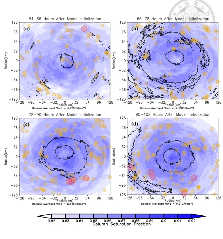
The snapshot of the composite averaged horizontal wind vectors, column saturation

fraction and the geometric center and size of VHTs of DS and NDS averaged every 12

hours in the 48 hours period prior genesis are given in Figure 4 and Figure 5. To compare

the occurrence of VHTs in a fair sample size, only the two experiments with the earliest

genesis time in the DS are plotted to compare the two experiment in the NDS. It is evident

that, DS have increasingly higher saturation fraction in a concentric region surrounding

the center of the vortex prior genesis. The occurrence of large VHTs with volume larger

than 10⁵km³ are also more frequent as time approaches genesis. The upscale growth of

VHTs to 10⁶km³ seems to initialize at the 3^rd quadrant of a concentric ring around 84-96

km from the vortex center. As time approaches genesis, the maximum occurrence of

VHTs propagates closer to the vortex center. This propagation is coherent with the

increase in the region of high saturation fraction. As the time approaches 0-12 hours

before genesis, the large VHTs are concentrated at the region with very high saturation

fraction (SF>0.9), approximately inside the 32 km circle of the vortex center.

Alternatively, the environment in NDS has smaller saturation fraction and lower

occurrence of large VHTs.

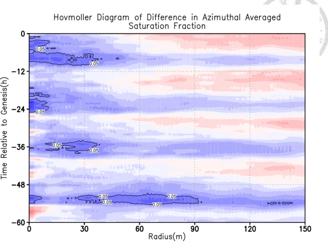
The Hovmöller diagram of the difference in azimuthally averaged saturation fraction

between DS and NDS are shown in Figure 6. The region in which DS have a moist

(30)

anomaly over 0.05 is contoured, as time approaches genesis, this region will propagate

closer to the center of the vortex. One of the prominent difference between DS and NDS

is the degree and position of column saturation, with DS moister in the innermost 100 km

region and dryer on the outside than NDS. A semi-diurnal variation of saturation fraction

is also observed.

(31)

Figure 4. Evolution of averaged composite saturation fraction, shown in shaded, geometric center and the size of VHT objects of h4v3 and h3v3 at the time period (a) 36-48 Hours (b) 24-36 (c) 12-24 (d) 0-12 hours prior genesis. The wind speed is contoured from 2.5-7.5 ms^-1, at an interval of every 2.5 ms^-1.

(a) (b)

(c) (d)

(32)

Figure 5. Same as Figure 4, but for NDS.

(a) (b)

(c) (d)

(33)

Figure 6. Hovmöller diagram of difference in azimuthally averaged saturation fraction between DS and NDS. Blue (red) denotes positive (negative) anomaly of DS relative to NDS. Positive anomaly that exceeds 0.05 is marked with contours.

(34)

3.3 Statistical properties of moist entropy

Chapter 3.1 shows that vortex achieves cyclogenesis in a shorter period when the

vortex is placed close to the mid-troposphere, and if the vortex is placed either too low or

too high, the vortex does not amplify in the selected time interval of 144 hours. The initial

vortices have similar strength and horizontal extents, but different perturbed potential

profiles caused by balance thermodynamic response. Chapter 3.2 qualitatively shows that

the spatial distribution of saturation fraction varies between DS and NDS , and the spatial

distribution, size and occurrence of convection is related to the spatial distribution of

saturation fraction. Cyclogenesis in the experiment is accompanied by column saturation

near the center of the vortex. To our knowledge, saturation fraction is controlled by the

large-scale variables such as domain averaged vertical profile of moist entropy.

Consequentially, the next logical step is to statistically evaluate if there is a systematic

difference in the environment of DS and NDS.

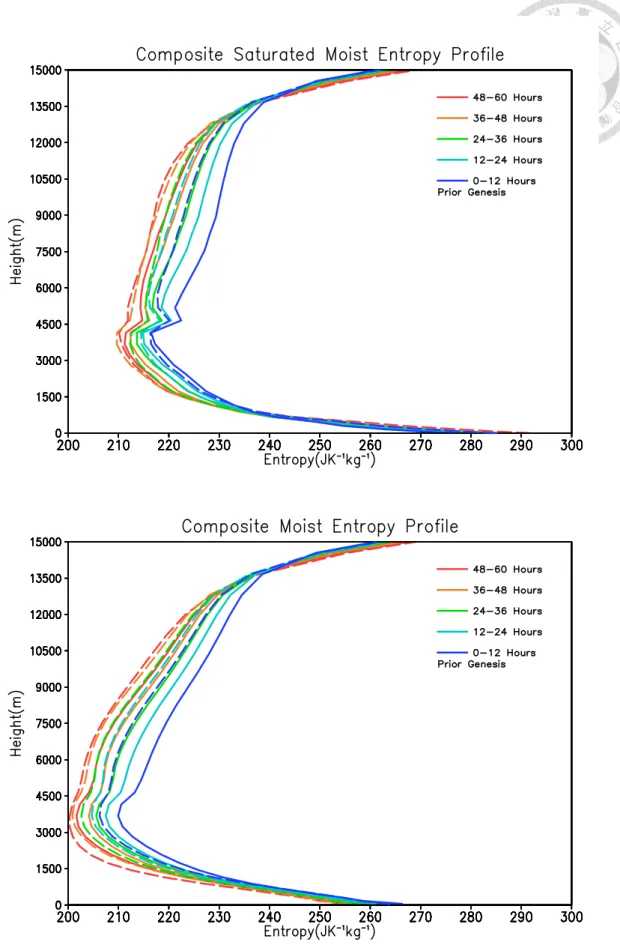
First we present the evolution of composite averaged vertical profile of moist entropy

and saturated moist entropy in a 100×100 km² box around the vortex center sampled every

12 hour period, prior to the the tg of DS and NDS sets in Figure 7. The saturated moist

entropy is larger in the DS than NDS above 4500m, with highest discrepancy from 5000m

to 12000m, and smaller in the DS than NDS below 1500m.

(35)

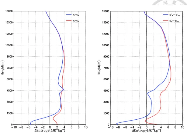
The difference is clearer if we subtract s and s* of DS and NDS 24-36 hours and 0-12

hours prior to the cyclogenesis, shown in Figure 8. It is evident that 24-36 hours prior

cyclogenesis, the DS already exhibits a negative(positive) s* anomaly compared to the

NDS at the lower(mid-upper) troposphere, showing a relative more stable troposphere

in the DS. As time approaches cyclogenesis, the negative anomaly of saturated moist

entropy below 1500m of troposphere further increases from 6 J K^-1kg^-1 to 8 J K^-1kg^-1

and positive anomaly increases from 4 J K^-1kg^-1 to 6 J K^-1kg^-1, showing further

stabilization. Hovmöller diagram of 𝑠_𝑑^∗ − 𝑠_𝑛𝑑^∗ (Figure 9) indicates that the anomalous

pattern is evident even 60 hours prior to the genesis. Increase in the difference of moist

entropy is especially prominent in the upper troposphere as time approaches genesis.

(36)

Figure 7. Evolution of averaged s* (top) and s (bottom) in a 100×100 km² box around the vortex center, indicated at the time interval. The solid lines are the DS and dashed line are the NDS.

(37)

Figure 8. Difference between averaged s (red) and s* (blue) in a 100×100 km² box of DS and NDS (∆𝑠 = sds - snds) 24-36 hours (left) and 0-12 hours (right) prior to cyclogenesis

Figure 9. Hovmöller diagram of sds* - snds*, the difference of saturated moist entropy between DS and NDS, abscissa denotes height in meters

(38)

We quantify the environmental stabilization using the idea based on Raymond et al.

(2014), the difference of averaged s* in [1,3] km (𝑠_𝑙𝑜𝑤^∗ ) and [7,9]km (𝑠_{ℎ𝑖𝑔ℎ}^∗ ):

Stability Index (𝑆𝐼) ≡ ∆𝑠^∗ = 𝑠_𝑙𝑜𝑤^∗ − 𝑠_{ℎ𝑖𝑔ℎ}^∗ (Eq. 8)

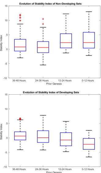
The box plot of SI sampled in a 100×100 km² box around the vortex center, binned by

every 12 hours from 48 hours prior to the genesis is shown in Figure 10. It is evident that

while the median is similar between two sets at 36-48 hours prior genesis, the distribution

of DS is skewed more towards the negative side and have a lower maximum value. As

time approaches 24 hours prior to the genesis, the median stability index of DS drops

substantially. At 24-36 hours prior genesis, median 𝑆𝐼 is around 0.53 Jkg^-1K^-1 more

stable than the NDS. The discrepancy further increases as time approaches 0-12 hours

prior to the genesis, when the median 𝑆𝐼 is around 4.51 Jkg^-1K^-1 more stable than the

NDS. Table 3 shows the values of each quantile of SI of DS and NDS.

One might ask why experiment h7v3, although posing a positive (negative) anomaly

of 𝜃 below(above) the PV maxima, still exhibits a lower stability index. This may be

due to the fact that negative 𝜃 extends too far into upper troposphere, leading to the

reduction in the difference in saturated moist entropy between the lower troposphere and

upper troposphere where our SI is defined.

(39)

Figure 10. Box plot of averaged SI at the interval stated in the abscissa, prior genesis, in a 100×100 km² box around the vortex center for NDS (top) and DS (bottom). The black bar denotes the extent of the maxima and minima. The blue box is the range between first quartile and third quartile. The red line denotes the median. The red cross denotes the outliers.

(40)

Stability index (J K^-1kg^-1)

36-48 Hours 24-36 Hours 12-24 Hours 0-12 Hours prior to the the genesis

DS NDS DS NDS DS NDS DS NDS

Minima -4.1346 -3.0208 -4.2123 -5.4939 -4.8059 -1.32 -6.6421 -2.2183 Q1 -0.6444 -0.6698 -1.6224 -1.2319 -2.7808 0.4038 -4.0332 0.3435 Median 0.6034 0.7481 0.0263 0.5545 -0.7797 2.2329 -2.2556 2.2659 Q3 2.0697 3.4073 2.5776 2.624 1.7765 5.3334 -0.2196 5.8358 Maxima 6.7913 11.9458 7.7701 10.4317 5.6762 12.2128 2.5803 12.953

3.4 Statistical properties of saturation fraction

The environmental saturation fraction (SF) have a few implications. According to

Raymond et al. (2009) and Raymond et al. (2007), precipitation rate under moisture quasi-

equilibrium exponentially increases as saturation fraction (column relative humidity)

increases. Column saturation is observed to precede genesis and this exponential relation

still holds in cyclogenetic environment (Wang & Hankes, 2016). If this is true, then the

associated increase in moisture convergence at the lower troposphere is required to

maintain this moisture quasi-equilibrium. Tsai and Wu (2017) proposed that as saturation

fraction exceeds a certain threshold, the probability distribution of convective clouds size

tends to exhibit a bimodal distribution where a there exist a second extrema in larger cloud Table 3. Quantiles of stability index averaged over 100×100 km² box around the vortex center sampled in

the given period.

(41)

sizes. The size difference between the modes will grow exponentially as the saturation

fraction increases.

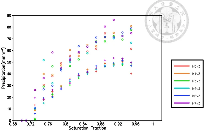
The scatter plot of the top 1% average and domain average of precipitation in a

100×100 km²box around the center of the vortex, binned by 0.02 of saturation fraction

is presented in Figure 11. Unlike aforementioned results, precipitation rate in our

experiment does not increase asymptotically as SF reaches a critical value. Nonetheless,

the consistent positive correlation between saturation fraction and precipitation in all of

the sensitivity experiments shows that the environment remains in a moisture quasi-

equilibrium state prior genesis.

The box plot of SF sampled in a 100×100km² box around the vortex center, binned by

every 12 hours period from 48 hours prior to the genesis is shown in Figure 12. There is

a systematic increase in the saturation fraction as time approaches genesis. Starting from

36-48 hours prior to the genesis, distribution of SF are comparable between the DS and

NDS. However, the maximum SF are larger and the distribution are right skewed in the

DS as opposed to the left skewness of NDS. As time approaches genesis, the median

saturation of DS increases to approximately 3% higher than NDS, and the distribution

narrows significantly showing that the grid points on the drier end at the previous time

periods becomes significantly moistened. It is evident that although the maxima and

median both increases in DS as time approaches genesis, it is the significant increase of

(42)

SF values in the drier end of SF that distinguishes DS from NDS, revealing that the

prominent feature of DS is the decrease in the areal occupation of drier patches. The

values of each quantiles are shown in Table 4.

(43)

Figure 11. Scatter plot of average precipitation in a 48 hours period prior to genesis of top 1% (open circle) and all samples (plus sign) in a 100×100 km² box around

the vortex center box, binned by saturation fraction of 0.02.

(44)

Figure 12. Box plot of area averaged SF sampled at the interval stated in the abscissa, prior genesis, in a 100×100 km² box around the vortex center for NDS (top) and DS (bottom)

(45)

Although the difference of 3% in median is somewhat nominal, if we look back to

Figure 4, the significant increase in saturation fraction that covers the large area within

the inner region of the system can create a substantial difference in the capability of

generating large, aggregated convective system in the spatial perspective.

Saturation Fraction

36-48 Hours 24-36 Hours 12-24 Hours 0-12 Hours Prior Genesis

DS NDS DS NDS DS NDS DS NDS

Minima 0.807 0.787 0.8293 0.7995 0.8331 0.7982 0.8468 0.8031 Q1 0.8391 0.8155 0.8452 0.8252 0.8496 0.8301 0.8608 0.831 Median 0.8475 0.8368 0.8542 0.8361 0.8607 0.8441 0.8678 0.8417

Q3 0.8639 0.8474 0.8649 0.8452 0.872 0.8568 0.8757 0.8554 Maxima 0.8817 0.8742 0.8825 0.8719 0.8874 0.8695 0.8872 0.8725

Table 4. Quantiles of saturation fraction averaged over 100×100 km² box around the vortex center sampled in the given period.

(46)

3.5 Relation between saturation fraction and stability index

We have shown that as time approaches cyclogenesis in DS, the environment stabilizes

through the warming of mid-upper troposphere and cooling of boundary layer, creating a

positive (negative) anomaly above (below) 1500m relative to NDS, followed by column

saturation. According to the hypothesis and observational studies of Raymond et al.

(2011), they proposed that in a cyclogenetic environment SF will be inversely

proportional to SI. The increase of saturation fraction is through the work of stabilization

that promotes “bottom heavy” convective mass flux profile, which converges moisture

from the lower-troposphere and transport upwards through intense vertical motion. The

log10-scaled joint PDF of SF and SI, sampled in the 100×100km² box around the vortex

center 0-48 hours prior genesis, is shown in Figure 13. Accordingly, we verify that in both

DS and NDS, SF is inversely proportional to SI, and the probability density is skewed

toward higher SF and lower SI for DS compared to NDS. The difference in probability

density between DS and NDS is shown in Figure 14. The probability in high SF-low SF

regime can be 4-10 times higher in DS than in NDS, indicating that an environment about

to undergo cyclogenesis is characterized by high SF and low SI. The contoured values are

the averaged precipitation rate (mmhr^-1) of each grid point in the joint-probability

distribution space, which clearly shows a positive proportionality between SF and

(47)

precipitation rate. It is worth noting that, there are some localized maxima of precipitation

in DS at the lower end of SF but extremely stabilized environment, a sign that some

convective activity may exist under extremely stabilized environment even if SF is low

in developing vortices.

(48)

Figure 13. Log10-scale joint probability distribution of column saturation fraction versus stability index of (a) DS and (b) NDS. Sample are taken from 0-48 hours prior genesis in a 100×100 km² box around the vortex center. The

average precipitation of each grid on the joint-probability space are contoured.

log10(P) log10(P)

(a)

(b)

(49)

Figure 14. The difference of log10 PDF between DS and NDS. Regime with difference in P>10^0.3 are marked with contour.

(50)

To inspect the details in the difference of proportionality between each sensitivity

experiment, scatter plot of averaged stability index versus saturation fraction, binned by

every 0.01 of saturation fraction is shown in Figure 15. The difference between the

sensitivity experiments within the DS and NDS are small. However, if we compare the

stability index between DS and NDS, there is clear discrepancy between the average

values of stability index between the two at higher saturation fraction, especially in the

time period 0-12 hours prior genesis. Here we explain this discrepancy by the vertical

integral of lateral entropy flux divergence on a cylindrical coordinate:

[∇ ⋅ (𝜌𝑣𝑠)] = [𝑠∇ ⋅ (𝜌𝑣)] + [𝑣 ⋅ ∇(𝜌𝑠)] = [𝜌𝑤^∂s

∂z] + [𝑣_𝑟^∂𝜌𝑠

r ∂r]

(

Eq. 9)

∇= ( ∂ r ∂r𝑟̂, ∂

∂z𝑧̂) where [𝐴] = ∫ 𝐴𝑑𝑧

The second equality is derived by applying mass continuity and integration by parts

on the first term on the RHS. In a weak incipient vortex, we assume the radial inflow is

weak and radial entropy gradient is small, the first term on the RHS will then dominant

[∇ ⋅ (𝜌𝒗𝑠)]. A troposphere with flatter vertical gradient of s, or smaller SI, given the same profile of vertical velocity, the value of 𝜌𝑤^𝜕𝑠

𝜕𝑧 is will be smaller in the mid-upper troposphere according to our definition of stability index, applying vertical integration,

this corresponds to less net divergence or more net convergence of moist entropy in a

vertical column. From Figure 16, we can see that the composite of azimuthally averaged,

(51)

vertically integrated flux divergence of moist entropy is indeed less than 0 in DS at the

region around the vortex averaged 0-12 hours prior genesis, indicating a net convergence

of moist entropy in these stabilized environment.

(52)

Figure 15. Scatter plot between SF and mean SI, binned by 0.01 interval, sampled during (a) 0-12 hours and (b)24-36 hours prior cyclogenesis in a 100×100 km² box around the vortex center. The dashed line denotes the averaged stability index for DS (red) and NDS (green).

(a)

(b)

(53)

Figure 16. Azimuthally averaged [∇ ⋅ (𝜌𝑣𝑠)] of DS (red) and NDS (green), averaged during 0- 12 hours period prior genesis.

(54)

Chapter IV. Impact of vortex-scale thermodynamic environment to cloud scale systems

4.1 Size and number of cloud and vortical hot tower (VHT)

Clouds are labeled and grouped as objects using the method discussed in 2.3.3. The time

series of domain wide cloud number and within a 100×100 km²box around the vortex

center is shown in Figure 17. The time series of domain wide VHT number and within a

100×100 km²box around the vortex center is shown in Figure 18. For both DS and NDS,

domain wide cloud number and VHTs decreases at a similar rate prior and post genesis.

On the other hand, the evolution of cloud and VHT number in a 100×100 km²box around

the vortex center of DS is clearly different than that of NDS. DS is characterized by cloud

number reaching maxima approximately 12 hours prior genesis, and then a substantial

drop in cloud number subsequently, whereas the tendency in cloud and VHT number of

NDS proceeds at a similar rate, showing no difference in the time period.

(55)

Figure 17. The (a) Domain Wide Cloud Object (b) Cloud Object Count in a 100×100 km² box around the vortex center. The data is low pass filtered to exclude half-day diurnal variations.

(a)

(b)

(56)

Figure 18. Same as Figure 17, but for the counts of VHTs (a)

(b)