Indexing for Dynamic Abstract Regions

(1)

Indexing for Dynamic Abstract Regions

Joxan Jaffar Roland H.C. Yap School of Computing National University of Singapore 3 Science Drive 2, 117543, Singapore {joxan, ryap}@comp.nus.edu.sg

Kenny Q. Zhu Microsoft Corporation

One Microsoft Way Redmond, WA 98052, USA kennyzhu@microsoft.com

Abstract

We propose a new main memory index structure for ab- stract regions (objects) which may heavily overlap, the RC- tree. These objects are “dynamic” and may have short life spans. The novelty is that rather than representing an ob- ject by its minimum bounding rectangle (MBR), possibly with pre-processed segmentation into many small MBRs, we use the actual shape of the object to maintain the in- dex. This saves significant space for objects with large spa- tial extents since pre-segmentation is not needed. We show that the query performance of RC-tree is much better than many indexing schemes on synthetic overlapping data sets.

The performance is also competitive on real-life GIS non- overlapping data sets.

1 Introduction

Indexing of spatial objects, objects with non-zero area or volume is an important traditional problem in databases.

In this paper, we want to consider a new class of applications where the spatial objects naturally overlap. Consider a stock portfolio management setting with a large number of traders and a constantly changing market. Stock brokers, liketradestation.com, already offer traders the ability to trade using triggers. Here, a trigger is a rule which de- fines an action to invoke when the rule condition is true.

Conditions are trader-defined constraints on stock prices, volumes, interest rate, cash, etc. Each active trader can have potentially many triggers. In a brokerage with lots of traders, the total number of triggers can be very large (tens of thousands). Given a market change, rather than at- tempting to evaluate all triggers, we use indexing to filter out irrelevant triggers.

The problem of efficiently determining the potential matching triggers can be cast as a query to a spatial index.

The objects to be indexed are abstract regions in a multi- dimensional space corresponding to the trigger conditions.

Figure 1. German roads (rectangles)

A query occurs whenever there is a market update which takes the form of a stabbing query, since the update is a multidimensional point. The abstract regions are expected to be geometric but in arbitrary shapes since they arise from conditions. Because traders may specify similar conditions, we expect that significant overlap of regions is possible. In contrast, GIS applications deal with spatial data which may have little or no overlap since they correspond to physical objects. The triggers here are also similar to, but often more complex than, those in active databases [23]. In active databases, since the number of rules is not very large, indexing is less of a problem.

Another feature of these applications is that objects are dynamic and transient, e.g. a day trader may add new trig- gers and remove old ones which may only last a few hours.

Thus, the index has to support dynamic object insertion and deletion. However, since market changes (queries) happen much more frequently (e.g. stock prices change constantly) than changes to the triggers (insert/delete), we focus on efficient queries over inserts/deletes.

Traditionally, the common representation to index spatial objects is a minimum bounding rectangle (MBR). An object is either represented by a single MBR or is segmented into a number of MBRs if it has large spatial extent. Segmentation is usually employed as a pre-processing step to the indexing algorithm. As a result, the original shape of the object is lost and not used in the indexing algorithm. Fig. 1 shows

(2)

an example where roads are pre-processed into many small MBRs in a GIS application. In a GIS context, as objects are permanent and have a clear usage, this is reasonable.

However, in applications with dynamic abstract regions, it is not feasible to determine the resolution of the segmentation in advance. Segmentations which are coarse introduce too much “dead space” while segmentations that are too fine would increase space and time costs unnecessarily.

Historically, indexes were stored in secondary storage.

This situation is changing with the advent of machines with large address spaces and large main memories [8]. Since the objects we are considering are mostly transient, main memory indexes is a reasonable and sound idea. This changes the context of the indexing problem since disk-based and in-memory indexing have different cost considerations. In disk-based indexing, the relevant measure is the number of I/O operations. For an in-memory index, more fine-grained measures such as the number of memory operations are meaningful. Hence the strategy of increasing the size of index nodes and fan-out, and decreasing the height of the tree in disk-based indexes may actually have a detrimental effect when applied to in-memory indexes.

A

d2 d3

d1

C B

Figure 2. Domain reduction and clipping In this paper, we introduce a novel in-memory data struc- ture called RC-tree (Reducible Clip-Tree) for indexing spa- tial objects. RC-tree combines three main ideas, namely:

object clipping, domain reduction and rebalancing. Like the R⁺-tree [21] and the quadtree [20], the RC-tree adopts a space-partitioning strategy. Informally, a discriminator is a hyperplane that partitions the space. An object intersecting with a discriminator is clipped into two parts. Due to the clipping, the MBRs of subtrees at the same level are disjoint, thus avoiding multiple traversals for point-queries.

The difference with the RC-tree is that it indexes the actual shapes of the original objects in addition to their MBRs.

Clipping is done on the original objects, and the (updated) MBRs of the two resulting sub-objects are used to replaced the original MBR. This way, the total size of the new MBRs are reduced, hence we call this domain reduction. The idea of domain reduction is illustrated in part (A) – (C) in Fig. 2.

Three objects drawn with thick lines are shown in part (A).

Part (B) depicts a single MBR representation (as in R-tree [9] without segmentation) for each object with the MBR drawn in dotted lines. The MBRs heavily overlap with a

lot of dead space. Point queries may have low accuracy since the overlapping MBRs would require searching multiple paths in the tree.

Domain reduction makes use of the discriminators created during the process of building or rebalancing the tree.

These discriminators dynamically produce MBR approximations by segmenting the indexed objects. In part (C), suppose the discriminators are d1, d2 and d3 shown with the dashed line. This results in six MBRs created by domain reduction. The MBRs have no overlap and have less dead space in (C) than in (B).

It is important to note that objects are segmented (clipped) only when there is a need to discriminate them based on the current tree. When the tree changes, the segmentation can also change. In contrast, a static MBR segmentation strategy can create too many or too few MBRs.

d1

d2 d3

L1 L2

d1 d1

d3

d2

d3

d2 L

L2 L1

d1

d2 d3

L L L L

RC−Tree Other Binary Clipping Based Tree

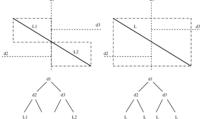
Figure 3. Advantage of domain reduction Domain reduction can also lead to space reduction over other space partitioning strategies. Consider RC-tree with another binary MBR-clipping-based search tree using the same clipping strategy in R⁺-tree. In Fig. 3, domain reduction of MBRs in RC-tree creates a tree with only two items (“L1” and “L2”) in the leaves, while the other tree has four items (denoted by “L”). Insertion cost is also less since RC-tree inserts two less objects.

RC-tree uses a binary general weight-balanced tree [1]

as its backbone. Rebalancing by partial rebuilding is done whenever a part of tree is out of balance. Rebalancing also serves another important purpose which is to control object clipping and space usage. It repartitions the original objects which reside in a given subtree by choosing a series of new discriminators. This would lead to a possibly different col- lection of MBRs and clipped objects.

In summary, the RC-tree takes advantage of the under- lying shapes of the objects, as well as their MBRs. Rather than using MBR approximations and processing the MBRs, the actual objects are indexed and partitioned dynamically.

Furthermore, the partitioning is performed in a lazy fashion,

(3)

that is, only when needed, depending on the current state of search tree structure. This avoids the space and time costs of partitioning when it is not needed. The RC-tree improves search behavior while avoiding problems and costs associated with pre-segmentation.

Our experiments on synthetic overlapping data sets show that RC-tree can significantly outperform R-tree variants (R, R^∗, R⁺) and PMR-quadtree [20] in terms of search cost comparisons and query accuracy. For non-overlapping real- life GIS data sets, the RC-tree is also very competitive.

2 Related Work

Most of the spatial indexing techniques use B-tree ap- proaches with large nodes and high fanout as the index is designed for secondary storage. R-trees [9] extend the B- tree ideas to multi-dimensional search trees. R^∗-trees [3]

improve the R-tree with a different node splitting algorithm.

Subsequently, there are many other R-tree variants [13]. Be- cause almost all R-tree variants allow the MBRs in the in- ternal nodes to overlap, a point query may have to traverse multiple paths of the tree, even when the data objects have no overlap! An exception is the PR-tree [2], which has a worst case optimal bound similar to the kd-tree, It is a hy- brid between R-tree and kd-tree and is a static index with special bulk loading and search algorithms.

The R⁺-tree [21] is different from other R-tree variants as it avoids the problem of having to search multiple paths by using disjoint MBRs and MBR clipping. The difference between clipping in R⁺-tree and RC-tree is: R⁺-tree clips intermediate MBRs and duplicates object MBRs, while RC- tree clips the actual objects applying domain reduction.

Most R-tree variants approximate and index the objects by MBRs. Such approximations can be very inaccurate for non-rectangular objects and give a higher query miss rate.

Some extensions of R-trees move away from MBR approximations. P-trees [10] use polygonal approximations, and SR-trees [11] use spheres as estimation. We are not aware of spatial structures that index the actual objects, as in RC- tree. Furthermore, RC-tree’s domain reduction technique, approximates sub-objects dynamically and on-demand.

Quadtrees also partitions space and clip objects. How- ever, quadtrees have a fixed branching factor and equal space partitions at the same level. While quadtrees were designed for point data, the PMR-quadtree [20] can store objects of arbitrary shapes such as line segments. Unlike RC-tree, quadtrees are not balanced.

Kd-trees [4] are binary trees originally designed for multi-dimensional point data. Extensions like Skd-tree [15]

and Matsuyama’s kd-tree [14] index non-zero size spatial objects by representing a spatial object by its centroid which is a point. They then behave like a kd-tree in partitioning the points. In the Skd-tree, overlapping partitioning of space

is possible, thus, multiple paths may be searched. Mat- sumaya’s tree duplicates an object whenever its MBR (in- stead of the object itself) intersects with a partition, and can lead to excessive duplication with large objects.

As there are many spatial indexing techniques, we refer the reader to the excellent survey by Gaede and Gunther [7]. Our approach revisits many of the issues in a new way, combining features of kd-trees, MBR clipping, domain reduction and partial tree rebuilding. We also provide ways for tuning the space-time tradeoff.

The way RC-tree dynamically segments objects to be indexed can be compared with the z-ordering with redun- dancy in [16]. Domain reduction is different from z- ordering with redundancy which has a predefined maximum resolution of segmentation, whereas the RC-tree dynamically determines object partitioning. It is also different since one is comparing a multi-dimensional index with a trans- formed one-dimensional index.

There is also other work on main memory R-tree indexes. CR-tree [12] is a cache-conscious version of R- tree. They show around two-times speed-up in search performance. The main idea in CR-tree is to quantize the MBR entries, which allows for a higher fanout for the same node size, with a given cache line size. This idea is implementation specific and is largely independent from the underlying algorithm. It can be applied to most index structures, in- cluding RC-tree. The CUR-Tree [19] is a cost-based unbalanced R-tree for main memory with cost functions to factor in a query distribution. The minimum filling factor constraint is removed so it is not height balanced.

3 The RC-Tree

A RC-tree is a general weight-balanced binary tree for efficient search and update of spatial objects in k−dimensional space. Every intermediate node of a RC- tree is a hyperplane that partitions the space assigned to this node. The space is thus divided into two sub-spaces. Ob- jects entirely contained in a sub-space belong to that sub- space; objects intersecting the hyperplane are clipped and the two resulting clipped objects stored in each sub-spaces.

The root node is assigned the entire space. The hyperplane (the discriminator) serves to discriminate objects in the two sub-spaces. Intermediate node in the tree contains the following: a discriminator hyperplane, the number of objects that are indexed under this node, and left/right pointers.

All original data objects, clipped or not, are stored in the leaf nodes. A leaf node can store one or more objects. A predefined leaf capacity L is associated with the RC-tree.

When a leaf node stores more objects than L, it is called an overflow node. Overflow nodes store objects as a set without any additional structure.

We model objects as a conjunction of constraints O, over

(4)

a subset of the k variables in the geometrical space. For example, a line segment l passing through the origin could be defined as: 2x + 3y = 0 ∧ −5 ≤ x ≤ 5

Discriminators are also modeled as a constraint, e.g.

x ≤ 8 is a discriminator that divides the whole space by a hyperplane x = 8. The constraint approach, similar to [22], provides a powerful mechanism for describing and using arbitrary geometric shapes and general discriminators.

If an object defined by O is contained in the left half-space of a discriminator d, we say O ⇒ d; if it is contained in the right half-space, we say O ⇒ ¬d. If an object O is clipped by d, the left-hand part is a new object O ∧ d, and the right- hand part is O ∧ ¬d. Every object has an MBR, which is the projections of O in each of the k dimensions.

A RC-tree T is called α-balanced, if the height of T ob- serves h(T ) ≤ (1 + α) log(|T |), where α ≥ 0, and |T | is the number of nodes in T . α-balancing is used to bound the height of the search tree to within a log factor.

3.1 RC-Tree Algorithms

Let T.d be the discriminator at node T , and |T | be the number of nodes under T . T.lef t (T.right) are the left (right) child and h(T ) is the height of the tree rooted at T . Algorithm Pack(S, T, Levels)

Input: A set of n unordered objects S; Levels to pack into Output: A weight-balanced RC-tree T of height log(n).

P1. Split(S, S1, S2, T );

P2. if Levels > 0 then

Pack(S1, T.lef t, Levels − 1);

Pack(S2, T.right, Levels − 1)

else make T a leaf (or overflow) node that contains S Levels is initialized to dlog(n)e. Pack bounds the tree height by log(n).

Algorithm Split(S, S1, S2, T) Input: A set of objects S

Output: Two sets of objects partitioned by d, and a tree node T defined by d and the MBR of S.

SP1. select a discriminator T.d using the partition procedure with an objective function f ; SP2. for each O ∈ S:

if O ⇒ T.d, then S1 := S1 ∪ {O}

else if O ⇒ ¬T.d, then S2 := S2 ∪ {O}

else S1 := S1 ∪ {O ∧ T.d};

S2 := S2 ∪ {O ∧ ¬T.d}

The choice of discriminator is controlled by the partition objective function which is a heuristic to balance discrimination versus clipping.

Algorithm Insert(T, O)

Input: An RC-tree rooted at T , a new object O Output: A new RC-tree rooted at T

I1. if T is not a leaf then

if O ⇒ T.d then Insert(T.lef t, O) else if O ⇒ ¬T.d then Insert(T.right, O) else Insert(T.lef t, O ∧ T.d);

Insert(T.right, O ∧ ¬T.d);

if h(T ) > (1 + α) log(|T |) then Rebuild(T ) I2. if T is a leaf node then

add O to T ;

if |T | > L, then for set of nodes S in T : Split(S, S1, S2, T );

create a child node T.lef t containing S1;

create a child node T.right containing S2 The leaf capacity, L, is a factor that can be tuned to af- fect the insertion cost and the space usage. A leaf node is split when it exceeds L objects. If there is no suitable dis- criminator, no splitting is done and the leaf node becomes an overflow node.

Algorithm Delete(T, O)

Input: RC-tree rooted at T with n objects, new object O Output: A new RC-tree rooted at T

D1. if delcount == 2^1+α^β ⁻¹n then Rebuild(T ); delcount := 0 else delcount := delcount + 1 D2. if T is not a leaf then

if O ⇒ T.d, then Delete(T.lef t, O) else if O ⇒ ¬T.d, then Delete(T.right, O) else Delete(T.lef t, O ∧ T.d);

Delete(T.right, O ∧ ¬T.d);

if |T.lef t| + |T.right| ≤ L then

extract the objects in T.lef t and T.right;

join the clipped parts and put them in a set S;

make a leaf node with objects in S D3. if T is a leaf node then Remove O from T

Every top level call to Delete initializes delcount to zero.

β is a constant to control the frequency of rebuilding [17].

Algorithm Search(T, W)

Input: An RC-tree rooted at T , a search window W Output: All objects that intersect W

S1. if T is not leaf then

if W ⇒ T.d then Search(T.lef t, W ) else if W ⇒ ¬T.d then Search(T.right, W )

(5)

else return Search(T.lef t, W ) ∪ Search(T.right, W )

S2. if T is leaf then return objects in T intersecting with W Algorithm Rebuild (T)

Input: An imbalanced subtree rooted at T Output: A balanced subtree rooted at T

T1. extract the set of all original objects from T into set S T2. Pack (S, T )

3.2 Discussion

3.2.1 MBRs for the intermediate nodes

To speed up the rejection of negative queries, we also add MBRs to the intermediate nodes in the RC-tree (not shown in Sec. 3.1). The MBR at any tree node covers all objects stored in its subtrees. Intermediate MBRs are updated as new objects are inserted or deleted from its subtrees. Our experiments show that adding these MBRs makes searching 70%-80% more efficient.

3.2.2 Partitioning

The partition procedure is used to find a suitable discriminator, hence is critical to the indexing performance. Ideally, we want a discriminator that balances the weights of two resulting sets of objects and minimizes the amount of clipping to minimize space utilization. The partitioning should also be fast. Since these goals are often conflicting, we propose two partitioning methods: RC-SWEEP uses an ob- jective function that combines the effect of weight balance and minimum clipping; RC-MID does fast partitioning and ignores balancing and clipping considerations.

RC-SWEEP sorts the given set of objects in each dimension in the space respectively. It adopts the plane sweep procedure similar to the one in the R⁺-tree. Candidates for discriminators are the boundaries from the MBRs of objects, these could have been already been clipped by domain re- duction. For each candidate discriminator d, we calculate a cost based on the following objective function:

f (d) = δ(nl+ nr− nd) + σ|nl− nr| (1) where nl(nr) is the number of objects that will go to the left (right) set respectively given discriminator d; and ndis the number of objects that are not clipped by d, or which do not intersect d. δ and σ are weights to adjust the cost function towards balance or minimization of clipping. After sweep- ing through all the possible candidates in all dimensions, we will pick a d that gives the minimum f (d) value.

RC-MID assumes that the MBR of the set of the objects is known in advance. This information can be computed

incrementally as objects are inserted. Let x be a dimension in which the MBR has the largest extent, and we select a d = (xlb + xub)/2, where xlb and xub are the lower and upper bound of the MBR in the x direction, respectively.

RC-MID gives a a fast discriminator but its effectiveness depends on the distribution of the objects.

It is not essential for the discriminators to be orthogonal.

An arbitrary hyperplanes/constraint can be used to partition the space. This is similar to the approach in Binary Space Partitioning (BSP) [6]. For efficiency reasons, we use orthogonal hyperplanes.

3.2.3 Partial rebuilding

The RC-tree uses a partial rebuilding technique first intro- duced by Overmars [17] to rebalance itself. After every Insertion(T , O), it checks against the balancing criterion of h(T⁰) ≤ (1 + α) log(|T⁰|), where h(T⁰) is the height of the new subtree rooted at T⁰after insertion. The balancing criterion ensures that the tree height is within a constant factor of the log of the number of nodes in the tree.

When the balance of RC-tree is broken, partial rebuild- ing finds the lowest node T in the tree where the balancing criterion is not satisfied. It “flushes” out all objects in the subtree into a list. If two objects belong to one original object, they are merged. Thus, at the end of the flush, there are n distinct objects in the list. Our algorithm sorts the ob- jects in all dimensions and then applies Split(S, S1, S2, T ) recursively to obtain a new, balanced tree. To speed up the process, the recursive split uses the same sorted list.

In deletion, a global rebuilding of the whole tree is done once enough deletes are done. More details on the approach can be found in [1, 17]. Rebuilding the entire tree is expensive, but it happens less frequently.

3.2.4 Space control

We use a space control factor γ to tune the space usage in the RC-tree. If total number of clipped objects in the sub-tree is greater than γn, further splitting is forbidden.

This means the algorithm P ack may terminate before the counter reaches log(n). If there are more than L objects in the leaf, this leaf becomes an overflow node.

4 Empirics

We show empirical comparisons of RC-tree (with different leaf capacities and with/without space control) against several R-tree variants and PMR-quadtree. The experiments were run on a Pentium 4 2.4GHz with 512M of RAM and Linux 2.4.20. Our RC-tree implementation is written in C++ and in the generalized constraint based style.

(6)

We compared the two RC-tree partitioning methods. Our experiments show that while RC-MID performs better in insertion cost, the space requirement is be much higher. As such, we will only show results with RC-SWEEP.

The R-tree and R^∗-tree are the C++ implementation by Marios Hadjieleftheriou. The R⁺-tree is adapted from the C implementation by Timos Sellis’ group. All these R-tree implementations can be found at [18] and are in-memory index implementations. For the R-tree family, we have used fanout sizes ranging from 3 to 50 for the index nodes, except for R^∗-tree, which used fanout 4 and above. We do not use R-tree variants with a node size of 2 as the tree is no longer balanced (in fact, the search becomes very expensive).

The PMR-quadtree is our own C implementation based on the algorithm in [20] with fanout 4 and a bucket sizes of 20 and 50. PMR-quadtree with smaller bucket sizes can- not handle some of our datasets due to memory exhaustion.

We control the height and the space of PMR-quadtree by restricting the minimum quadrant size to a 0.1 × 0.1 cell.

Figure 4. Schematic of rand (lines)

Figure 5. Schematic of grid (triangles) Given that we have various implementations in different languages which may not be optimized, timing is not an ac- curate measure of cost. Furthermore, we want a uniform fine-grained measure which makes sense for in-memory algorithms. To this end, we will use the number of discriminators or MBRs compared/tested which is the dominant op- eration in the algorithms in a main memory context. We denote this measure as accesses.

In the graphs below, RC(x) denotes an RC-tree with leaf

capacity x and no space control, and RC(SC) denotes an RC-tree with leaf capacity 1 and space control γ = 1.3.

In all RC-trees, the balancing factor α is 0.9. R(x) de- notes an R-tree using quadratic splitting with node size x.

Quadratic splitting is used since the search performance is usually better than linear splitting without sacrificing too much on insertion cost [3]. We remark that the node size is important as it affects space usage and performance. With an in-memory structure, it does not make sense to use large nodes because the cost of processing a node is linear in the node size. PMR-quadtree is denoted as QT (x), where x is the bucket size. In the experiments of Sec. 4.1 and 4.2, we have used random point queries. The number of queries in each data set is equal to the number of objects in that data set.

Space usage is measured by counting the total number of nodes multiplied by the number of floating numbers needed to represent the discriminator/MBR in each node. The sizes for pointers are ignored here which underestimates the space usage for the R-tree family when node size increases.

4.1 Synthetic overlapping objects

We first compare the search/insertion/space performance of RC-tree with other indexes on synthetic datasets with objects consisting of line segments or triangles. Lines and triangles are chosen as they are about the simplest geometric shapes in real-life applications. The datasets are as follows:

• rand(0/1): uniformly distributed objects of variable sizes, see Fig. 4.

• clust(5/10): variable-size objects around 5 or 10 clus- ters

• grid(2/3): variable-size objects placed systematically in a grid pattern, see Fig. 5.

The number after rand and grid denotes the degree of overlapping, i.e. rand1 has more overlap than rand0. Fig. 4 and 5 illustrates the patterns of the datasets. However, the actual layout of the objects in these datasets are much denser:

each problem has 50,000 objects of sizes ranging from 100 to 500, within an area of 10000 × 10000.

We remark that these synthetic datasets are meant to be reasonable as they consist of objects with various degrees of local overlap. They are not chosen to be pathologically bad for the competing methods. For the sake of fairness, we have avoided objects with excessively large spatial extent or dead space as RC-tree would have even greater advantage.

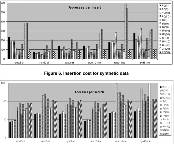
Insertion cost, as expected, is higher for RC-tree than most other methods primarily due to rebuilding. We observe in Fig. 6 that increasing leaf capacity reduces the insertion cost for both RC-tree and PMR-quadtree, though the same does not hold for R-tree family. The results show that space

(7)

Figure 6. Insertion cost for synthetic data

Figure 7. Search cost for synthetic data (log scale)

control is also useful as a strategy for controlling the insertion cost. The insertion cost is lowest at R(10) and R^∗(10) and it increases for R⁺-tree as fanout increases.

Fig. 7 uses a log scale. It shows that RC-tree has uniformly better query performance over the other methods.

RC-tree is at least three times better, and in many cases such as R-tree (rand1-line) and R⁺-tree (grid3-line), more than ten times. The insertion cost savings from increased leaf capacity comes at a price in search cost for almost all methods.

The general trend is that larger nodes means more expensive search. In general, the search cost of R-trees increases significantly as fanout increases. In the case of rand1 and grid3 which have high MBR overlap, the advantage of clipping- based methods such as RC and QT over the non-clipping methods is obvious. This suggests that space partitioning is a desirable when it comes to indexing overlapping spatial regions.

With lines and triangles, RC-tree stores the actual object shapes rather than its MBRs alone. When there is heavy overlapping, RC-tree tends to clip more in order to obtain better object discrimination but at a cost of more space.

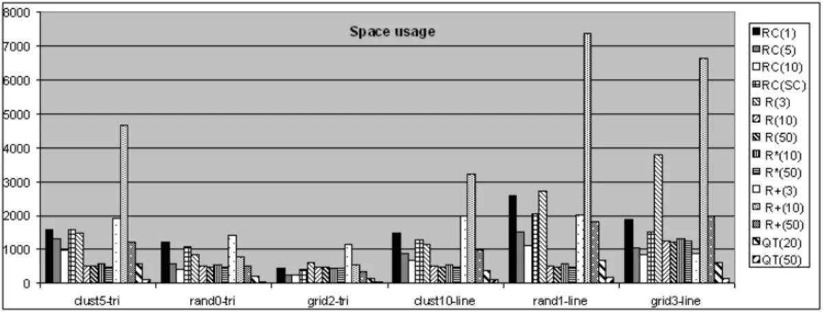
Fig. 8 compares the space cost of the various algorithms

and RC-tree strategies. We see that RC-tree manages the space-time tradeoff better than R⁺-tree which can be more than one order of magnitude worse. This may explain why R⁺-tree seems not to be used in practice since space costs can be high. RC-tree, by contrast, varies from being comparable to 2-3 times more than R-trees. This shows that domain reduction is able to reduce the size of the MBRs of clipped objects on the fly and hence reduce tree size (Fig.

3), whereas storing only the MBRs in R⁺-tree does not have such effect. The space control and increased leaf capacity in RC-tree also help in making the space usage of RC-tree competitive. We note that increasing the bucket size significantly reduces the space for PMR-quadtree without significant penalty in search performance. Large bucket sizes cause less clipping, hence, better space efficiency. Since the data sets here have some uniform random distribution, quadtrees with large bucket sizes are also shorter and more balanced. The search within a large bucket offsets the ben- efit of a smaller (and more balanced) tree.

(8)

Figure 8. Space usage for synthetic data (’000 numbers) 4.2 Non-overlapping rectangular datasets

We now investigate the performance of RC(1) with the other methods on traditional GIS data sets. The following data sets are made up of small pre-segmented rectangles that have little or no overlap (the number of rectangles are indi- cated in brackets): roads (30674) (Fig. 1), rrlines (36334), rivers (24650) and hypsogr (76999). We remark that these data sets are real-life GIS data and can be found at [18].

Figure 9. Insertion cost on GIS datasets

Figure 10. Search cost on GIS datasets

Figure 11. Space usage: GIS datasets (’000 numbers)

From figures 9, 10 and 11, we find that, with a mod- erately high insertion cost tradeoff, the RC-tree has much better search performance with comparable space usage to the R-tree family. This is interesting since RC-tree is not intended for indexing rectangles which the domain of R- trees. The space usage of RC-tree is small for rectangle data largely because the partial rebalancing technique helps maintain the tree in more balanced shape than its counter- parts. We can see in Fig. 11 that R⁺-tree incurs too much space overhead for small node sizes. However, the space overhead for R⁺-tree with larger node sizes is competitive.

It is only when the overlap increases, as in the synthetic data sets, the R⁺-tree space overhead can become prohibitive.

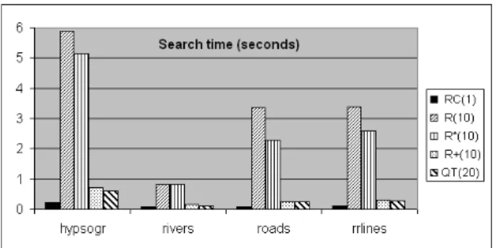
Finally, as a sanity check for actual running times, we compare the wall clock query time of RC(1) with the best performing variants in all other methods on the GIS datasets. We remark that the running times is not a fair comparison since the different implementations are in a mix of C and C++ and may not be optimized. Our RC-tree implementation is certainly not optimized as it uses generalized constraint discriminators which can be replaced in a OO- style plus the C++ code would not be as efficient as opti-

(9)

Figure 12. Search cost (wall clock time) mized C code. With these caveats, the results in Fig. 12 are consistent with the access cost measure.

4.3 Query accuracy and range queries

Figure 13. Hit rates on synthetic and GIS datasets (negative log scale)

Fig. 13 compares query accuracy across indexing methods where accuracy is defined as (shorter bars are better)

hit rate = number of hits

number hits + number of misses For the GIS datasets, RC-tree is significantly better, in some cases by several orders of magnitude. The hypsogr dataset is chosen as being representative as the performance advantage of RC-tree is quite similar across all the GIS datasets.

For synthetic datasets, one would expect that the probabil- ity of getting a hit is increased with highly overlapping regions. Thus, Clust5-tri with large areas of overlap, shows a smaller difference in hit rates among the methods. We see that RC-tree has uniformly better accuracy across all methods. We conjecture that keeping actual shapes and domain reduction helps reduce dead space and the dynamic decom- position with clipping gives better discrimination.

Although our motivation for RC-tree focuses on point queries, our algorithm also handles range queries. Table 1 compares range query performance across the methods.

“Size” in Table 1 refers to dimensions of the query window

starting with a point query. RC(1) is compared with the best performing methods: R family with node size 10 and QT(20) on the two data sets, roads and rand0-tri. The first number in every cell is the average search cost, and the per- centage is the hit rate. Table 1 demonstrates that the advan- tages of RC-tree also apply in range queries. As the query window increases in size, we expect that accuracy increases for all methods as shown.

roads

Size 0 20 40 60 80 100

RC 12.5 15.5 19.7 25. 0 31.6 39.4

(1) 62.9% 86.5% 92.1% 94.3% 95.7% 96.6%

R 36.8 39.8 43.3 47.1 51.4 56

(10) 2.9% 11.6% 20.7% 28.3% 34.8% 40.4%

R^∗ 31 33.6 36.7 40.2 44.1 48.5

(10) 3.6% 13.9% 24.1% 32.2% 39.2% 44.9%

R⁺ 37.4 45.5 54.4 63.6 73.6 84.2

(10) 1.3% 5.65% 10.1% 14.0% 17.4% 20.4%

QT 82.6 86.1 90.2 94.7 99.8 105.4

(20) 0.9% 5.2% 11.1% 17% 22.6% 27.8%

rand0-tri

Size 0 20 40 60 80 100

RC 21.1 29.1 39.4 52.0 66.5 83.7

(1) 14.8% 39.5% 53.3% 62.3% 68.5% 73%

R 162.2 170.9 179.9 189.4 199.4 209.8 (10) 1.8% 4.6% 7.5% 10.4% 13.3% 16.1%

R^∗ 62.0 67.2 72.9 79.0 85.6 92.6

(10) 4.9% 11.3% 17.1% 22.4% 27.2% 31.5%

R⁺ 44.7 51.4 59.1 68.0 77.8 88.8

(10) 6.8% 15.7% 22.8% 28.3% 32.7% 36.2%

QT 90.4 96.6 103.8 111.9 121 131

(20) 5.9% 15.5% 24.3% 31.84% 38.1% 43.4%

Table 1. Range queries (accesses/hit rates)

Seg. Misses Search Insert Space

RC 1 17327 18.32 110.0 185.9K

R(3) 4.2 18483 58.5 53.4 399.5K R(5) 16.7 18233 85.9 46.8 1.03M R(10) 62.5 20189 164.3 62.1 3.6M R^∗(5) 16.7 16391 199.1 216.4 1.2M R^∗(10) 62.5 16752 71.1 91.9 3.6M R⁺(3) 3.3 16606 35.7 100.6 733.2K R⁺(5) 10 17985 34.55 66.82 832.7K R⁺(10) 100 33310 49.82 74.25 4.58M QT(10) 100 20860 63.5 61.9 3.28M Table 2. Dynamic vs. static segmentation

4.4 Dynamic vs. static segmentation

To demonstrate the advantage of dynamic segmentation in RC-tree compared with static pre-segmentation used in

(10)

MBR-based indexes. we conducted the following experi- ment. We index in RC-tree 5000 randomly positioned line segments of the same length (500) in a 10000 × 10000 area.

We record the number of misses given by the RC-tree with 5000 random point queries, which is 17327. Then for every other index, we segment the given lines by cutting the line segments into smaller equal pieces and index the MBRs of the segmented pieces, such that the number misses is close to the RC-tree one. Essentially, we study the amount of segmentation needed and the associated costs of various indexes when a certain query accuracy is demanded. Table 2 records these results. The second column under “Seg.” in the table records the average number of pieces each object in the original dataset is segmented into. For example, for R⁺(5) to achieve misses of 17985, the original data have to be cut into 10 pieces each. The 4^th, 5^thand last columns record search, insertion and space costs. The results show that other indexes incur more space and search cost and, in some cases insertion cost as well, to get the same query accuracy as RC-tree. For R⁺(10), we were not able to achieve the same number of misses without exhausting memory.

60 80 100 120 140 160 180 200 220 240 260

11.5 12 12.5 13 13.5 14 14.5 15 15.5

Number of accesses

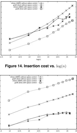
log(n) rrlines (MBR) without space control

grid5 (line) without space control rrlines (MBR) with space control grid5 (line) with space control

Figure 14. Insertion cost vs. log(n)

15 16 17 18 19 20 21 22 23 24 25

11.5 12 12.5 13 13.5 14 14.5 15 15.5

Number of accesses

log(n) rrlines (MBR) without space control

grid5 (line) without space control rrlines (MBR) with space control grid5 (line) with space control

Figure 15. Search cost vs. log(n)

4.5 Insertion and query cost vs. data size

To investigate the relationship between insertion/search costs and the number of objects, we pick two datasets, rrlines and grid5, whose scaling factor s is roughly con- stant against n. We run the insertion and search algorithms of RC-tree on the first 4000, 8000, 12000 objects and so on. Fig. 14 indicates that there is almost a linear correlation between the insertion cost and log(n). Fig. 15 shows that as n goes large in rrlines, the search cost is no longer pro- portional to log(n), but sub-linear to it. A careful check re- veals the anomaly is because of the large empty space in the dataset. This causes many queries to fail, especially when n is small. Thus, when n is small, the search cost is under- estimated. Fig. 14 and 15 also show results from RC-tree with space control. Space control improves insert efficiency because less splitting and clipping is done, but the flip side is that more objects are stored in the overflow nodes, and hence they have to be searched in linear order. As a result, the search cost increases.

5 Conclusion

In this paper, we demonstrate that the RC-tree is a new clipping-based spatial index which can give very good search performance in main memory when compared with a number of common spatial indexes. The RC-tree is particu- larly good when the spatial objects have significant overlap.

It is also competitive for traditional non-overlapping scenar- ios. Furthermore, the RC-tree allows control over the time and space tradeoff. One can tune for more space and less time, or vice versa. The key to the success of the RC-tree is that it combines dynamic segmentation, domain reduction and partial rebuilding with tunable heuristics.

This paper, we believe, also breathes new life into indexing techniques based on space partitioning and object clipping. Due to concerns of space costs, such techniques have received little attention since R⁺-tree. Our results show this space problem does exist in R⁺-tree. However, with RC-tree, we show that a space partitioning index can enjoy superior query performance when indexing overlapping objects and at the same time have competitive space efficiency.

The use of dynamic segmentation also helps in reducing the space requirements by only clipping when needed.

References

[1] A. Andersson. General balanced trees. Journal of Al- gorithms, 30(1):1–18, 1999.

[2] L. Arge, M. de Berg, H. J. Haverkort, and K. Yi. The priority R-Tree: A practically efficient and worst-case

(11)

optimal r-tree. In Proceedings of the 2004 ACM SIG- MOD Conference, pages 347–358. ACM, 2004.

[3] N. Beckmann, H.-P. Kriegel, R. Schneider, and B. Seeger. The R*-tree: An efficient and robust access method for points and rectangles. In Proceedings of ACM SIGMOD Conference on Management of Data, pages 322–331. ACM, 1990.

[4] J. L. Bentley. Multidimensional binary search trees used for associative searching. Communications of the ACM, 18:509–517, 1975.

[5] M. Frigo, C. E. Leiserson, H. Prokop, and S. Ra- machandran. Cache-oblivious algorithms. In Proceed- ings of the 40st Annual Symposium on Foundations of Computer Science, FOCS 1999, pages 285–298. IEEE Computer Society, 1999.

[6] H. Fuchs, Z. Kedem, and B. Naylor. On visible surface generation by a priori tree structures. In Proceedings of SIGGRAPH ’80, Computer Graphics, pages 124–

133, 1980.

[7] V. Gaede and O. Gunther. Multidimensional access methods. ACM Computing Surveys, 30(2):170–231, June 1998.

[8] J. Gray and M. Compton. A call to arms. ACM Queue, 3(3), April 2005.

[9] A. Guttman. R-trees - a dynamic index structure for spatial searching. In Proceedings of ACM SIGMOD Conference on Management of Data, pages 47–57.

ACM, 1984.

[10] H. Jagadish. Spatial search with polyhedra. In Pro- ceedings of 6th IEEE International Conference on Data Engineering, ICDE, pages 311–319, 1990.

[11] N. Katayama and S. Satoh. The SR-tree: an index structure for high-dimensional nearest neighbor queries. In Proceedings of the 1997 ACM SIGMOD in- ternational conference on Management of data, pages 369–380. ACM, 1997.

[12] K. Kim, S. K. Cha, and K. Kwon. Optimizing multi- dimensional index trees for main memory access. In Proceedings of the 2001 ACM SIGMOD Conference.

ACM, 2001.

[13] Y. Manolopoulos, A. Nanopoulos, A. N. Papadopou- los, and Y. Theodoridis. R-trees have grown every- where.

[14] T. Matsuyama, L. V. Hao, and M. Nagao. A file organization for geographic information systems

based on spatial proximity. International Journal of Computater Vision, Graphic and Image Processing, 26(3):303–318, 1984.

[15] B. Ooi, K. Mcdonell, and R. Sacks-Davis. Spatial kd- tree: An indexing mechanism for spatial databases. In Proceedings of the IEEE Computer Software and Ap- plications Conference, pages 433–438, 1987.

[16] J. A. Orenstein. A comparison of spatial query processing techniques for native and parameter spaces. In Proceedings of the ACM SIGMOD Con- ference, pages 343–352, 1990.

[17] M. H. Overmars. The design of dynamic data struc- ture. Springer-Verlag, 1983.

[18] R-Tree Portal. http://www.rtreeportal.org.

[19] K. A. Ross, I. Sitzmann, and P. J. Stuckey. Cost-based unbalanced R-trees. In Proceedings of the 13th Inter- national Conference on Scientific and Statistical Data- base Management, pages 203–212, 2001.

[20] H. Samet. The Design and Analysis of Spatial Data Structures. Addison-Wesley, 1990.

[21] T. Sellis, N. Roussopoulos, and C. Faloutosos. The R+-tree: A dynamic index for multi-dimensional ob- jects. In Proceedings of the 13th VLDB Conference, pages 507–518. VLDB, 1987.

[22] P. J. Stuckey. Constraint search tree. In Logic Pro- gramming, Proceedings of the Fourteens International Conferences on Logic Programming, ICLP, pages 301–315. MIT Press, 1997.

[23] J. Widom and S. Ceri. Active Database Systems: Trig- gers and Rules for Advanced Database Processing.

Morgan Kaufmann Publishers, Inc., 1996.