國立臺灣大學電機資訊學院電機工程學系 碩士論文
Department of Electrical Engineering
College of Electrical Engineering and Computer Science
National Taiwan University Master Thesis
利用立體攝影機進行色彩與深度感測以達成三維環境 重建及物體追蹤
Three-Dimensional Environment Reconstruction and Object Tracking Using RGB-D Sensing of Stereo Camera
洪中易 Chung-Yi Hung
指導教授:連豊力 博士 Advisor: Feng-Li Lian, Ph.D.
中華民國一百零二年七月
July 2013
口試委員會審定書
誌謝
於臺大兩年的碩士生涯即將結束,這期間中學習及收穫良多,並且不論是在 課業、研究及生活上,受到的幫助相當多。最要感謝的是指導老師連豊力博士,
在這兩年的耐心教導與提醒,對於研究上需秉持細心及謹慎的態度,並從不同角 度及深度看待問題點,進而建立一套有系統的研究方法,以及從聽者的角度設計 圖像化簡報。這些訓練不僅在研究上有很大的幫助,相信未來處理任何事情,秉 持相同的態度及方法,也能夠迎刃而解;很感謝三位口試委員簡忠漢博士、李後 燦博士及黃正民博士耐心地聆聽,並給予相當多寶貴的建議,使本論文能夠更加 完善。
感謝 NCSLab 充滿活力且有趣的成員們陪伴,使這兩年研究時光相當充實。
感謝志明學長,時常給予研究的想法以及親切的鼓勵,使我在研究及撰寫論文時 能夠有所進展;感謝意淳學姊,打理實驗室的大小事務,並給予犀利的想法,讓 我能夠從更廣的角度來思考研究或是生活上面臨的問題;感謝多才多藝的俊兆學 長,每次聊天都有莫名其妙好笑的梗跑出來;感謝敬凱學長,在剛推甄上臺大時,
熱心推薦 NCSLab。詼諧又霸氣的個性帶給實驗室不少樂趣,也讓許多活動能夠順 利進行;感謝峻瑜學長,在碩零時帶著我使用立體攝影機,並且給予研究上一些 啟發。炒麵是 NCSLab 最難忘的回憶;感謝豐池學長,帶點台味的風格很趣味,
是每次歡唱都少不了的 NCS 男高音;感謝峯鳴學長,不論在研究、工作、玩樂及 待人處世上都是值得效仿的對象;感謝志祥學長,給了我很多程式上的建議;感 謝俊安學長,在討論或是 Meeting 過程中帶來的影像處理分析的知識及建議。也謝 謝學長詳細的課程筆記,讓我在上課時能夠更快進入狀況;感謝兩位同學在這段 期間一起奮鬥:感謝很有自制力的飛竑,在課業和研究上都是我們三人中的最佳 典範。在機器人學上,給予我相當多的知識和建議,使我在陌生的領域下,能夠 順利接軌;感謝凱翔,在這幾個月一起度過熬夜奮鬥的夜晚,讓我驚見人類體能 的極限。熱血不拘小節的性格,帶給實驗室相當多的歡樂及話題,並時常一起打 籃球,使我的球技增進不少;感謝實驗室的新血們,讓碩士生活更加精采。感謝 用歌聲征服 NCSLab 的柏逸,教我吉他並擔任實驗室的攝影師;感謝兆良,繼執 中學長後讓我再一次看到正拳魂;感謝俊榮教我使用雷射測距儀;感謝詠政教我 使用 Kinect,並提供金門特產還有團購餅乾;感謝家維,每次討論都使我獲益良多,
並讓我體認到後浪的可怕。
最後,感謝我的家人們,給予我無私的包容以及付出,使我能夠心無旁騖地 學習並完成論文;謝謝女朋友慶安,在這兩年的陪伴及關心,並體諒我的忙碌。
在此,僅以本論文,獻給所有幫助過我的師長及親朋好友們,謝謝大家。
洪中易 謹誌
利用立體攝影機進行色彩與深度感測以達成三維環境 重建及物體追蹤
研 究 生: 洪中易 指導教授: 連豊力 博士
國立台灣大學 電機工程學系
中文摘要
三維環境重建是目前一項熱門且應用廣泛的議題,諸如室內環境導覽、虛擬 實境以及微創手術之影像導覽系統。立體攝影機同時提供色彩及空間資訊,相較 於雷射僅提供空間資訊或單一攝影機提供色彩資訊,更能完整描述環境狀態,提 供充足的資訊於三維重建任務上。若能精確地將每一時刻攝影機的相對轉換關係 估算出來,立體攝影機量測點便能夠放置在正確的世界座標上,進而建立出三為 環境模型。因此首要的任務是利用連續影像上相同特徵點達成立體攝影機的定位。
然而,由於立體攝影機的不確定性及錯誤特徵點匹配,不將離群匹配點剃除直接 估測攝影機相對姿態將導致定位不精確或是錯誤估測。因此,隨機抽樣一致演算 法在此論文中用來作為離群匹配對的剃除。另一方面,由於立體攝影機為被動式 感測器,在許多情況如低紋理及光滑材質下,視差影像將產生許多破碎區域,影 響三維重建所需的資訊量。因此本論文將提出一個資料前處理的方法,降低量測 破碎,進而提高空間重建的品質。
此外,考量到動態環境下建置靜態地圖時,必須將動態物偵測出並將其濾除。
因此本論文提出了一套物體偵測及追蹤演算法,以機率形式建立佔據網格地圖擷 取出候選物體。接著,候選物體利用 HSV 色彩模型中的色相及飽和度分佈相似性 對應到正確的資料庫物體,以解決資料關聯性問題。最後,物體狀態的更新以本 論文所提出的更新策略搭配卡爾曼濾波器來達成。實驗結果顯示此系統能夠同時 追蹤多重物體,即使物體在一段時間超出攝影機視野或是被遮擋後再被偵測,仍 能夠準確追蹤。
關鍵字: 立體攝影機,RGB-D 定位,三維環境重建,物體追蹤,基於可視度之佔 據網格。
Three-Dimensional Environment Reconstruction and Object Tracking Using RGB-D Sensing of Stereo Camera
Student: Chung-Yi Hung Advisor: Dr. Feng-Li Lian
Department of Electrical Engineering National Taiwan University
ABSTRACT
Three-dimensional environment reconstruction is a key technology that has been widely researched over the last decade and has many applications such as indoor environment navigation, virtual reality and visual guidance system for minimal invasive surgery. Stereo camera provides color and spatial information together and therefore is more suitable in 3D environment reconstruction task than other sensors like laser range finder that only provides spatial information or mono camera that only provides color information. Once each camera relative pose is estimated precisely, measurement points provided from stereo camera can be placed at the correct position in the global
coordinate to reconstruct the 3D environment model. Thus, the most important task is to achieve the goal of localizing the camera pose by using the same feature points in the consecutive frames. However, because of the uncertainty caused by the stereo camera noise and the feature point mismatching, estimating the camera pose directly without eliminating the outliers could lead to an inaccurate or wrong result. Therefore, Random Sample Consensus (RANSAC) algorithm is applied to solve the outlier problem in this thesis. On the other hand, because of the limitation of the passive type sensor like stereo camera, the disparity map has many missing data areas that occur in several situations such as measuring object in low textureness or glossy surface. This problem may affect the quality of the reconstructed 3D model. Thus, the data preprocessing method is proposed to enhance the 3D reconstruction quality by reducing the missing data areas.
In addition, considering 3D model reconstruction task in dynamic scene, moving object needs to be detected and removed. Therefore, the object detection and tracking method is proposed to detect an object by constructing the occupancy grid map in probability representation to extract object candidate. Then the distributions of hue and saturation in HSV color space are used to link the candidate to the corresponding database object correctly to solve the data association problem. Finally, the proposed update strategy with Kalman filter is used to renew object states. The experiment results
an object is out of the field of view for a while or is in occlusion, the object can still be tracked correctly.
Keywords:
Stereo camera, RGB-D localization, 3D environment reconstruction, object tracking, visibility-based occupancy grid.
Contents
中文摘要 ... i
ABSTRACT ... iii
Contents ... vi
List of Figures ...viii
List of Tables ... xii
Chapter 1 ... 1
1.1 Motivation ... 1
1.2 Problem Formulation ... 4
1.3 Contribution ... 6
1.4 Organization of the Thesis ... 8
Chapter 2 ... 9
2.1 Three-Dimensional Environment Reconstruction ... 9
2.2 Object Detection and Tracking ... 13
Chapter 3 ... 18
3.1 Pin-hole Camera Model ... 18
3.2 Random Sample Consensus ... 20
3.3 Image Processing and Description ... 23
3.3.1 HSV Color Space ... 23
3.3.2 Morphological Image Processing ... 23
3.3.3 Connected-Component Labeling ... 28
3.4 Radial Basis Function ... 30
Chapter 4 ... 33
4.1 Stereo Camera Localization and Mapping ... 34
4.1.1 Feature Point Extraction ... 39
4.1.2 Feature Point Matching in Two Consecutive Frames... 43
4.1.3 Estimate the relative transformation matrix of rigid body by Least-Squares method using SVD. ... 46
4.1.4 Camera Pose Estimation with RANSAC Outlier Rejection ... 51
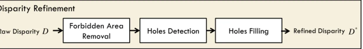
4.2 Stereo Vision Refinement ... 58
4.2.2 Holes Detection ... 66
4.2.3 Dual Orthogonal Linear Interpolation ... 68
4.2.4 Radial Basis Function ... 71
Chapter 5 ... 74
5.1 System Architecture ... 74
5.2 Object Detection ... 76
5.2.1 Visibility-Based U-Disparity Occupancy Grid... 77
5.2.2 Post-processing ... 85
5.2.3 Object Candidates Bounding Box Extraction ... 89
5.3 Object Tracking ... 91
5.3.1 Remove Background Pixels in Bounding Box ... 91
5.3.2 Registration between Candidates and Objects using Feature Vectors ... 93
5.3.3 Update Strategy with Kalman Filter ... 102
Chapter 6 ... 107
6.1 Experimental Hardware ... 107
6.2 Stereo Camera Localization and Mapping ... 112
6.2.1 Experimental Scenario Setup ... 112
6.2.2 The Effect of RANSAC Outlier Rejection Algorithm ... 116
6.2.3 Relation between Localization Accuracy and Mapping Quality ... 118
6.2.4 The Accuracy of Feature-based Localization Algorithm... 122
6.2.5 Three-Dimensional Reconstruction ... 125
6.2.6 Mapping Quality and the Proposed Stereo Refinement Algorithm Evaluation ... 129
6.2.7 Evaluate the Proposed Stereo Refinement in Spatial Aspect ... 135
6.3 Object Detection and Tracking ... 148
6.3.1 Object Detection ... 150
6.3.2 Object Tracking ... 156
Chapter 7 ... 167
7.1 Conclusion ... 167
7.2 Future Work ... 168
References ... 171
List of Figures
Figure 1.1: RGB-D data structure... 3
Figure 1.2: RGB-D data comparison between stereo camera and Kinect in an outdoor environment. ... 4
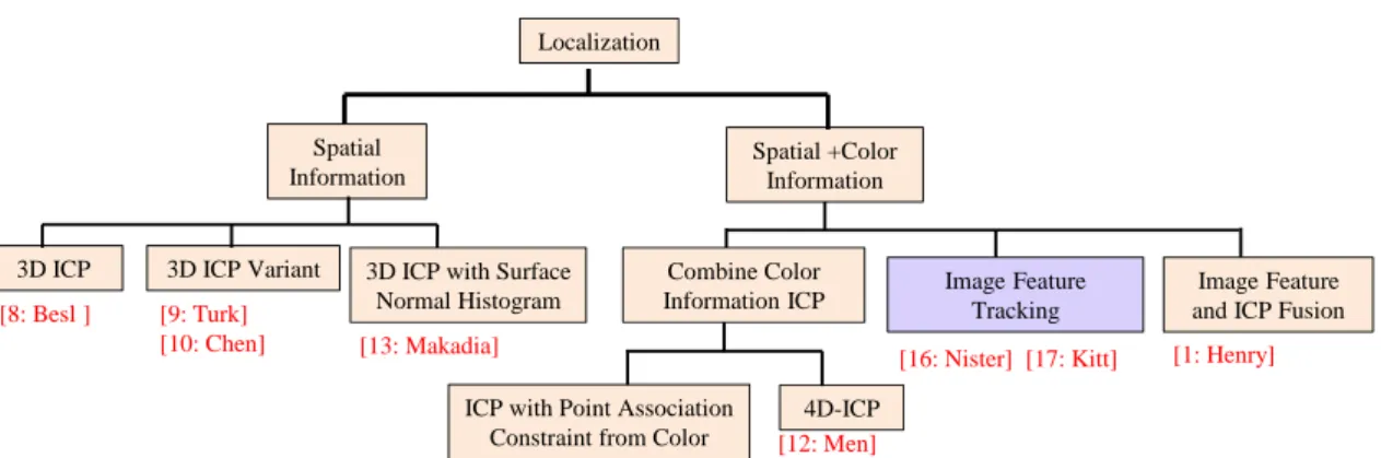
Figure 2.1: Sensor localization categories. ... 12
Figure 2.2: The object detection and tracking categories. ... 17
Figure 3.1: Illustration of pin-hole model ... 19
Figure 3.2: Example of RANSAC algorithm. ... 21
Figure 3.3: The illustration of the definition of reflection and translation. ... 24
Figure 3.4: (a) Binary image. (b) Square structure element (SE) with size 3 3× ... 25
Figure 3.5: Process of dilation operator in each step. ... 26
Figure 3.6: Process of erosion operator. ... 27
Figure 3.7: Illustration of connected component Labeling for 4-connectivity. ... 30
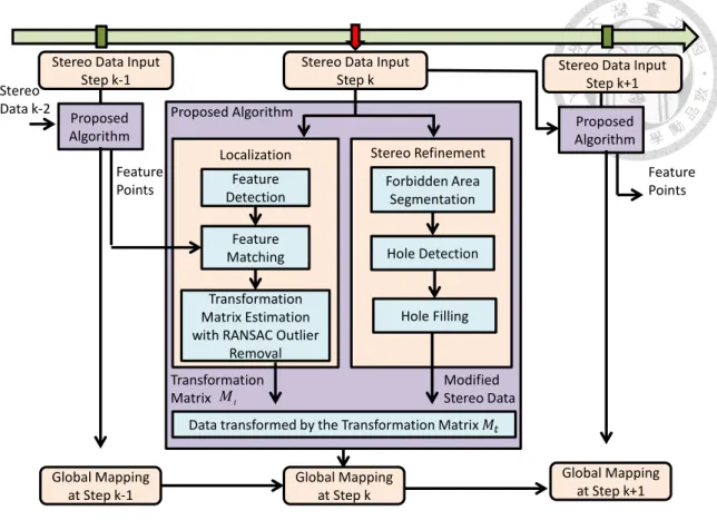
Figure 4.1: The proposed system architecture. ... 34
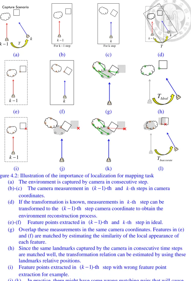
Figure 4.2: Illustration of the importance of localization for mapping task ... 37
Figure 4.3: The overall feature-based localization algorithm flowchart. ... 38
Figure 4.4: An example of spatial feature: Normal Aligned Radial Feature (NARF). ... 40
Figure 4.5: The flowchart of feature extraction ... 41
Figure 4.6: Feature extraction by SIFT detector ... 42
Figure 4.7: Block diagram of feature matching processing ... 44
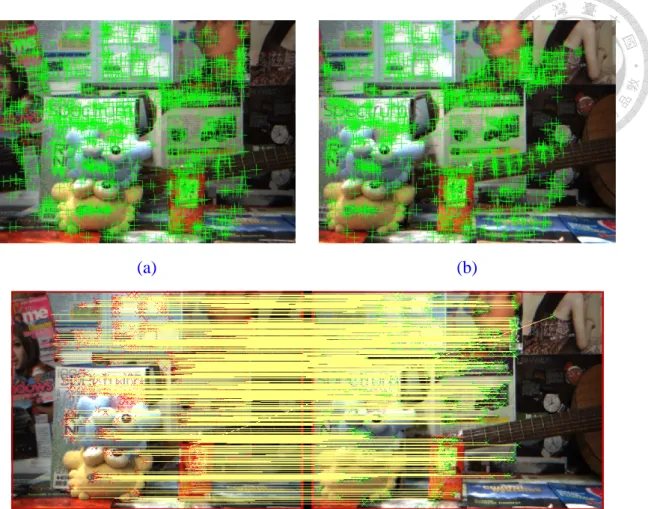
Figure 4.8: The result of feature matching by estimate the similarity between two feature descriptor. ... 45
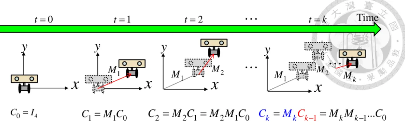
Figure 4.9: Illustration of two point sets with a certain motion. ... 49
Figure 4.10: Illustration of the relation between camera pose and relative camera motion. ... 51
Figure 4.11: Illustration of estimating the relative motion with RANSAC algorithm by two iterations for example. Green circles indicate the feature points in (k−1)-th step, while the red dots indicate the feature points in k-th step. Feature points in k-th step are projected by pin-hole camera model with certain transformation matrix. ... 56
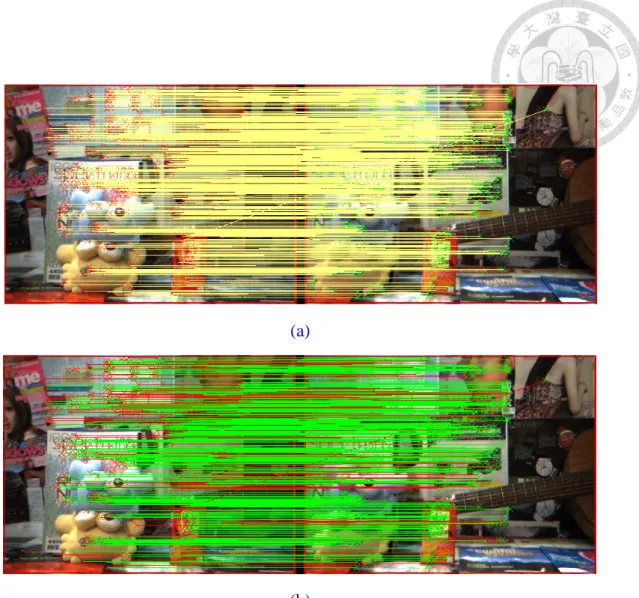
Figure 4.12: The result of using RANSAC outlier rejection algorithm on the matching pairs. ... 57
Figure 4.13: The block diagram of the proposed stereo refinement algorithm ... 58
Figure 4.14: Illustration of the occlusion area that out of the field of view (FOV) of left image plane ... 60
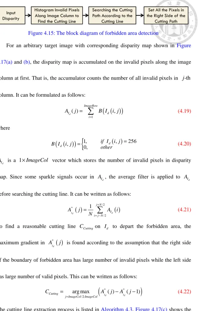
Figure 4.15: The block diagram of forbidden area detection ... 61
Figure 4.16: Illustrate the basic concept of the cutting path extraction according to cutting line. ... 64
Figure 4.17: The illustration of the proposed forbidden area detection ... 65
Figure 4.18: The flowchart of holes detection ... 67
Figure 4.19: Illustration of the hole detection concept ... 67
Figure 4.21: Illustration of the smallest bounding box extraction of a certain hole. ... 72
Figure 4.22: An example of filling a certain hole using radial basis function interpolation. ... 73
Figure 5.1: The proposed object detection and tracking system ... 75
Figure 5.2: Illustration of the visibility-based occupancy grid construction method... 79
Figure 5.3: Another example to illustrate the concept of the visibility-based occupancy grid map. ... 80
Figure 5.4: Each post-processing step applies to the u-disparity occupancy grid. ... 88
Figure 5.5: Illustration of bounding box extratction from u-disparity obstacle grid. ... 90
Figure 5.6: Background Pixels Removal for frame #236. ... 92
Figure 5.7: The registration result of each candidate to the database object. Different objects are enclosed by different color bounding boxes ... 95
Figure 5.8: Properties of object 1 in frame 236 ... 96
Figure 5.9: Properties of object 1 in frame 191 ... 97
Figure 5.10: HSV histogram of object 2 in frame 236 ... 98
Figure 5.11: Properties of object 1 in frame 237 ... 99
Figure 5.12: Properties of object 2 in frame 237 ... 100
Figure 5.13: A radius distance threshold for the possible range of the object candidates. ... 101
Figure 5.14: The proposed object update flowchart. ... 105
Figure 5.15: Two cases of unsuccessful object registration since no measurement in current step. ... 106
Figure 5.16: Checking if the object is out of the camera field of view (FOV). ... 106
Figure 6.1: A brief introduction of Bumblebee2 BB2-03S2-60 stereo camera. ... 109
Figure 6.2: IEEE 1394 Interface ... 110
Figure 6.3: Hokuyo URG-04LX-UG01 and SICK LMS100 laser range finders. ... 111
Figure 6.4: Experiment scenario ... 113
Figure 6.5: Experiment platform and accessories. ... 114
Figure 6.6: Camera path and corresponding image captured from right CCD ... 114
Figure 6.7: Horizontal laser data. The camera horizontal motion is estimated by applying ICP method to align two consecutive laser data. ... 115
Figure 6.8: Vertical laser data ... 115
Figure 6.9: Comparing the result of using feature-based localization method with and without RANSAC outlier removal. ... 117
Figure 6.10: Top view of the camera path. Red cross signs represent the positions estimated by laser-ICP; blue square signs indicate the positions estimated by stereo camera feature-based localization method; green star signs show the given command positions. ... 120
Figure 6.11: Translation and rotation error comparing to laser scanner ... 120
Figure 6.12: Laser data mapping with localization by stereo feature-based localization method and the given commands. ... 121
Figure 6.13: Stereo featured-based localization comparing to laser scanners. ... 123
Figure 6.14: Absolute translation error comparing to laser range finder. ... 124
Figure 6.15: Accumulate distance for moving 18 steps. ... 124
Figure 6.16: The mapping results in each step with two time interval. ... 126
Figure 6.17: Result of the three-dimensional environment ... 127
Figure 6.18: The local views of the reconstruction results at the same camera viewpoint. ... 128
Figure 6.19: The 3D model projects to image plane with certain camera poses ... 132
Figure 6.20: Illustration of the concept of using PSNR as similarity index to compare the 3D reconstruction quality in the color space viewpoint. ... 132
Figure 6.21: Comparing the 3D reconstruction result in different case. ... 133
Figure 6.22: Valid pixels projected from 3D model with and without applying the proposed stereo refinement method. White area in (a) and (b) indicate the valid pixel, while black region represent the pixels without valid value. ... 133
Figure 6.23: Experiment scenario setup. A plane stands in front of the stereo camera with different view angle. ... 138
Figure 6.24: The target image and the corresponding depth map of Data #3. ... 138
Figure 6.25: Two orthogonal laser data and transformed to camera coordinate. The local laser data is used to be the input of plane estimation. ... 139
Figure 6.26: Using local laser data to estimate the plane parameters ... 140
Figure 6.27: Comparing raw depth map and the depth map generated from the plane. ... 140
Figure 6.28: The 200 200× rectangular ROI is selected, which is enclosed as in the depth maps. ... 141
Figure 6.29: The absolute error between the depth of interpolating pixels and the depth generated from laser data. Red lines represent the result of the dual orthogonal linear interpolation approach, while the blue lines indicate the result of radial basis function method. ... 142
Figure 6.30: The data #1 interpolation result of two different approaches. ... 143
Figure 6.31: The data #2 interpolation result of two different approaches. ... 144
Figure 6.32: The data #3 interpolation result of two different approaches. ... 145
Figure 6.33: The data #4 interpolation result of two different approaches. ... 146
Figure 6.34: The data #5 interpolation result of two different approaches. ... 147
Figure 6.35: Experimental scenario setup ... 148
Figure 6.36: Experimental scenario setup ... 149
Figure 6.37: Detection rate of each object. ... 152
Figure 6.38: An example of histogram-of-oriented gradients (HOG) method failure detection case. ... 152
Figure 6.39: For the near range object, one of two cases that is considered to be false detection for example. ... 153
Figure 6.40: For the near range object, one of two cases that is considered to be false detection for example. ... 154
Figure 6.41: The far coming object not only has the false detection cases of entering the image plane and the occlusion, it also has the case that is too far to be detected. ... 155
Figure 6.43: Object tracking result with applying Kalman filter ... 159
Figure 6.44: Object tracking result without applying Kalman filter ... 159
Figure 6.45: Too close objects are measured as the same candidate in frame 60. ... 160
Figure 6.46: The candidate in frame 60 without Kalman filter ... 161
Figure 6.47: Position of object #1 with and without Kalman Filter ... 162
Figure 6.48: Position of object #2 with and without Kalman Filter ... 162
Figure 6.49: Position of object #3 with and without Kalman Filter ... 162
Figure 6.50: The path is divided into three parts. ... 164
Figure 6.51: Near path object tracking result comparing to laser. ... 166
Figure 6.52: Far path object tracking result comparing to laser. ... 166
Figure 6.53: Circular path object tracking result comparing to laser. ... 166
List of Tables
Table 4.1: Notations Definition ... 38
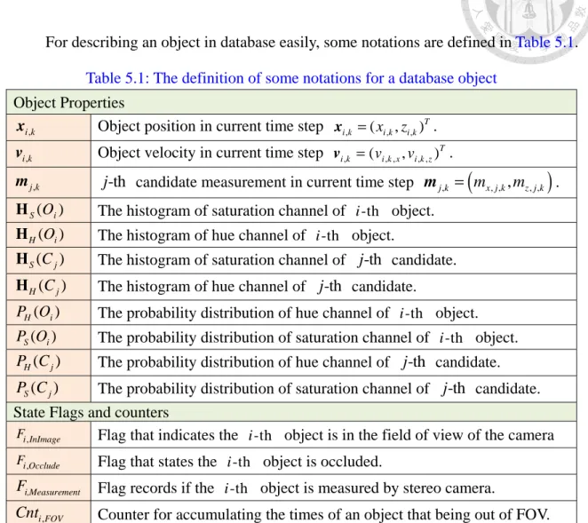
Table 5.1: The definition of some notations for a database object ... 76
Table 5.2: Bounding conditions of P O( U |V CU, U) ... 82
Table 6.1: The specification of stereo camera BB2-03S2-60 ... 110
Table 6.2: The specification of Hokuyo URG-04LX-UG01 ... 111
Table 6.3: The specification of SICK LMS100 ... 111
Table 6.4: 3D model projected to image plane and compare to target image. ... 134
Table 6.5: The mean and standard deviation of interpolation errors comparing to laser scanner (m). ... 142
Table 6.6: Comparing the processing time with different interpolation approaches. ... 142
Table 6.7: Successful detection rate of each object. ... 152
Table 6.8: The tracking result of near path (m) ... 164
Table 6.9: The tracking result of far path (m) ... 165
Table 6.10: The tracking result of circular path (m) ... 165
Chapter 1 Introduction
1.1 Motivation
Three-dimensional object and environment model reconstruction is a popular topic that has been researched in the last decade and plays an important role in many area such as robot navigation [1: Henry et al. 2012], virtual reality [2: Marcincin et al. 2012]
and visual guidance system for minimal invasive surgery [3: Park et al. 2012].
To build a 3-D model, not only the spatial information of an object is needed but also the color information. If the system only has spatial information, the model shape is built without knowing its appearance. Contrarily, if the system has only color information, the model cannot be reconstructed since the points cannot be placed in the correct positions. It shows the importance of color-spatial data structure for 3-D model reconstruction task. Recently, many sensors that have the ability to acquire color-spatial data have been developed, such as stereo camera and Microsoft Kinect. Both of them provide RGB color image and the corresponding disparity map (depth map) with same image coordinate, and this data structure is named as RGB-D data [5: Zeisl et al. 2012].
Moreover, RGB-D data can be extended to a RGBXYZ data structure, as shown in Figure 1.1. Therefore, the whole environment 3D model can be reconstructed by several
frame data capturing in different positions. In addition, Kinect is an active type sensor and its range image is acquired from the IR module, which is sensitive to incident angle and sunlight [6: Suarez et al. 2012]. Contrarily, Stereo camera is a passive type sensor and its range image is estimated by block matching algorithm, and do not have incident angle problem and is less sensitive to sunlight. Figure 1.2 shows the RGB-D data acquired from stereo camera and Kinect in outdoor environment. It is obvious to observe that the number of valid pixels in stereo depth map is larger than the number of valid pixels in Kinect depth map. Hence, stereo camera which belongs to passive type sensor is used in this thesis.
To place these points to the correct positions in the global coordinate, estimating the camera pose in each step is necessary, which is often called localization task. Many existing methods used to localize stereo camera pose have been developed, and one of these approaches is based on tracking the 3-D coordinate of image features and is often called “visual odometry” [16: Scaramuzza et al. 2011].
Although the environment 3D model can be reconstructed by the localization method which tracks the image feature points, many problems still need to be solved.
One of the problems affects the mapping quality is the shortcoming of stereo camera itself. The disparity map generated from two CCDs of the stereo camera by local
“brok ortho funct
abov witho probl consi conse 3D m dyna the s objec
ken holes.”
ogonal linea tion (RBF)
On the othe ve method.
out removin lems: First, idered to ecutive data model seve amic points, states of obj ct, the point
” To fix t ar (DOL) in
interpolatio er hand, it i However, i ng the dyna , the dynam
be the ou a frames tw eral times,
, this thesis bject. Once ts on the obj
these missi nterpolation on method in
is suitable t if the envir amic points mic points utliers; Seco wice or mor
causing the s proposed
the states o ject can be
Figure 1.1:
ing data, t n is propose
n the experi to reconstru
ronment is s in the mea will affect ond, these re, therefore
e ghost eff the object d of objects a
seen as dyn
: RGB-D da
the interpol ed and is co
iment in Ch uct 3D static a dynamic asurement d the localiz dynamic e, these poin fect. In ord
detection an are known, namic point
ata structure
lation meth ompared to hapter 6.
c environme c scenario,
data frames zation resul
points may nts will be er to detec nd tracking such as the s and be rem
e
hod called o the radial
ent model b build the m will cause lt since the ay occur in
mapped int ct and avoi g system to
e velocity o moved.
dual basis
by the model s two ey are n the to the
d the track of the
(a) (b) (c) (d)
(e) (f) (g) (h) Figure 1.2: RGB-D data comparison between stereo camera and Kinect in an outdoor
environment.
(a)(b)(e)(f) Color image and depth map from stereo camera.
(c)(d)(g)(h) Color image and depth map from Kinect.
1.2 Problem Formulation
In order to construct 3-D environment model by RGB-D measurements acquired at different positions, the sensor poses in each step need to be known. If the camera poses are known ideally, the data points with RGBXYZ structure can be placed to the correct positions with corresponding colors. However, these sensor poses are usually unknown in practice and need to be estimated. Many researchers investigated the six degrees of freedom sensor poses estimation by aligning two point clouds in k and k−1 steps using ICP and ICP variant methods. However, due to the uncertainty of stereo camera, it is not suitable to use ICP and ICP variant directly. Moreover, ICP needs a suitable initial
into local minimum. Contrarily, since camera moves step by step, many same feature points captured in the consecutive frames. By using the relative 3D coordinates of these points, the camera relative pose can be estimated by least-square method without any initial guess. However, two challenges need to be solved. First, features may not be linked correctly from previous to current frame, considering these wrong matching pairs in motion estimation may cause inaccurate or wrong result. Secondly, due to the sensor uncertainty, point may have inaccurate 3D coordinate, and will also affect the motion estimation result. These two cases are considered to be the outliers, and will be solved by applying Random Sample Consensus (RANSAC) algorithm.
On the other hand, stereo camera is a passive sensor, which the disparity map is generated by finding the same features from reference to target images, which is sensitive to illumination and textureness. This cause many missing data in the disparity map and therefore affects the mapping quality to the 3D models. To overcome the problem, this thesis proposes a data interpolation method to fix the missing data area efficiently by the average of the horizontal and vertical linear interpolation results.
Besides, considering 3D model reconstruction task in a real life scenario, many moving objects that do not belong to the 3D model need to be filtered out. Therefore, the object detection and tracking system is proposed. Many researchers have investigated object detection and tracking based on stereo vision, especially in the field
of intelligent transportation system (ITS). However, these tracking systems used in the traffic scenario do not need to consider tracking an object correctly in the cases of the object returning back to the camera field of view or partially occluded. Therefore, this thesis proposed the object registration method based on color distributions in HSV color space and the update strategy to update the object states to solve the data association problem during the system encounter the cases of object returning back to the camera FOV or partially occluded.
1.3 Contribution
The main contribution of this thesis is that the existing image feature-based localization method, the proposed stereo refinement algorithm, the visibility-grid map construction method proposed in [29: Perrollaz et al. 2012], the proposed object detection method and object tracking algorithm are combined together to achieve two main goals which are three-dimensional environment reconstruction and object tracking using stereo camera.
For the first topic, static environment reconstruction can be divided into two parts, which are sensor localization and stereo data refinement. For the first part, the existing feature-based localization method with RANSAC outlier rejection to achieve the goal of
six degrees of freedom (6-DoF) camera pose estimation [16: Scaramuzza et al. 2011] is integrated in this thesis. After finishing the localization step, each point measured by stereo camera can be added into 3D global model at the correct position with its color, and thus the 3D environment model can then be constructed. However, since many missing data in stereo camera, the proposed stereo refinement method combining with forbidden area elimination, missing data (hole) detection and hole filling is applied to fix this missing data area.
The second topic is the proposed object detection and tracking system. To detect object candidates from stereo camera data, the existing visibility-based occupancy grid map in u-disparity space [29: Perrollaz et al. 2012] with a slightly modification is integrated with the proposed post-processing algorithm in thesis. After object candidates are extracted, the next problem is how to link candidates to the database objects correctly. This problem is so called data association, and is solved by comparing the distributions of hue and saturation channels of the corresponding image patch in HSV color space with the proposed background pixels elimination method. Finally, to update the states of database objects in different cases, this thesis proposed an update strategy to handle the problem with Kalman filter.
The proposed systems can not only be used on stereo camera but also on other sensors which provide the same RGB-D data structure.
1.4 Organization of the Thesis
This thesis has 7 chapters including Chapter 1. The remaining part of this thesis is organized as follows: Literature survey is presented in Chapter 2. The related algorithms are discussed in Chapter 3. Two main parts of this thesis are discussed in the following two chapters. The three-dimensional environment reconstruction methods are shown in Chapter 4, including sensor localization and data refinement algorithms. In Chapter 5, object detection and tracking algorithms are presented. The experimental result and analysis are shown in Chapter 6. In the end of this thesis, the conclusion and future works are presented in Chapter 7 to show the benefits of the main ideas of the proposed system and point out some disadvantages that will be improved and extended.
Chapter 2
Background and Literature Review
2.1 Three-Dimensional Environment Reconstruction
In the last decade, many researchers have been investigated on how to reconstruct an environment map precisely using RGB-D sensor. According to the work in [1: Henry et al. 2012], to build a 3D environment map completely, a mapping system should
consider three components, which are spatial alignment (localization), close loop detection and global consistency.
For the first component, which is spatial alignment, is the most important element for mapping system to localize the sensor poses. As mentioned in Section 1.3, if sensor does not know its position accurately, the measurements from the sensor cannot map to the correct positions in the 3D global model. Many existing ways to align two consecutive data frames have been developed to achieve the goal of localization method.
The traditional and most popular way to align two point clouds is Iterative Closest Point (ICP) method [9: Bsel et al. 1992]. In the ICP registration algorithm, closest point in different point clouds is associated to compute the optimal rigid transformation iteratively that minimizes the mean-square error of each associated point between two datasets. However, due to noise points in the range data that affect the correctness of
point association, many ICP variant related techniques are proposed to solve this problem. For example, [10: Turk et al. 1994] proposed the point pairs elimination mechanism to remove point pairs that are too far apart or either points locates on a mesh boundary to avoid the outliers effect. [11: Chen et al. 1991] proposed point-to-plane error metric instead of point-to-point and get a better result on two surfaces registration.
Both of these two variant methods only consider the spatial information. For sensors that generate color point cloud, performing ICP with color constraint can solve the data association problem more convenient. For example, [12: Johnson et al. 1997] proposed the point pairs elimination using hue (the hue channel of HSV color space) of each points as a filter to be a constraint during the closest point search in every ICP iteration.
In [13: Men et al. 2011], the method not only consider the hue of each point as an elimination constraint, but includes the hue into the error metric as 4D-ICP, which the 4D means the , , -coordinatex y z and an additional hue intensity. Although many ICP variant algorithms solve the data association problem, both the above ICP and ICP variant algorithms are suffered from initial guess problem since ICP method aligns two data sets to the local minimum. To solve the initial guess, Makadia [14: Makadia et al.
2006] proposed the method to automatically estimate the initial guess and refine the
alignment by translating point cloud surface normal vector distribution into orientation
image feature-based localization, which is often called visual odometry, are the most popular to RGB-D type sensors since the initial guess can be easily solved by using the image feature such as Scalar Invariant Feature Transform (SIFT) [20: Lowe 2004] or Speeded-Up Robust Features (SURF) as landmarks [16: Scaramuzza et al. 2011].
However, because many outliers such as wrong feature matching pairs affect the pose estimation result, Random Sample Consensus (RANSAC) outlier rejection algorithm is applied to solve this problem [17: Nister et al. 2004]. Moreover, for binocular stereo vision, since two image planes are fixed, the feature coordinates in reference image plane can be a constraint to check the correctness of each matching pairs of the target image plane in feature matching step. This concept was proposed in [18: Kitt et al.
2010], using the so called trifocal tensor to describe the relationship between three
images (which are the two images from previous step and the target image in current step). Besides, [1: Henry et al. 2012] proposed two stage RGB-D localization method by fusing feature tracking with RANSAC outlier rejection and ICP. However, the authors claim that feature-based method is good enough and applying ICP can refine the result slightly. Since image feature-based localization with RANSAC can solve the initial guess and outlier rejection to get a precise localization result and is easily implemented, this thesis chooses this method to achieve to goal of localization.
For the second and third components, which are close loop detection and global
consistency, are used to minimize the error during the frame-by-frame localization. To detect close loop data frames, keyframes are selected and are compared in each data frame [1: Henry et al. 2012]. After detect the close loop, some optimization methods are used to minimize the error. For example, in [1: Henry et al. 2012], two methods are implemented to compare the results: the first method is tree-based network optimizer (TORO) which uses stochastic gradient descent to maximize the likelihood of node parameters subject to the constraints; another is sparse bundle adjustment (SBA), which globally minimize the re-projection error of feature points which are matched in all data frames. Loop detection and global consistency are essential when reconstructing large scale environment model. However, the scenarios in this thesis do not encounter loop closure and global consistency and these problems are considered to be the future works.
Figure 2.1: Sensor localization categories.
Localization
Spatial Information
Spatial +Color Information
3D ICP Combine Color
Information ICP Image Feature
and ICP Fusion 3D ICP with Surface
Normal Histogram
4D-ICP ICP with Point Association
Constraint from Color [12: Men]
[8: Besl ]
[13: Makadia] [1: Henry]
[11: Johnson]
3D ICP Variant [9: Turk]
[10: Chen]
Image Feature Tracking [16: Nister] [17: Kitt]
2.2 Object Detection and Tracking
Object detection tracking have been researched for a long time and have been developed by different sensors. According to the properties of different sensors, the object detection task can be categorized into two types, beam-type sensor based and vision-based. For the first category, beam-type sensor, such as laser range finder or ultrasound, provides spatial information by returning an environment point positions. In [34: Wolf et al. 2004], the authors proposed the moving object detection method by
constructing a static grid map, and comparing each scan data to this static gird to filter out the dynamic points. However, tracking laser points are a challenge problem, since no other information to determine how to link an object point to the object in next scan correctly. It is well known as data association problem [62: Thrun 2005]. Although many hypothesis approaches have been developed to overcome the problem, considering only spatial information to solve data association problem is still hard and makes ambiguous result.
On the other hand, for vision-base category, it can be divided into mono camera and RGB-D type sensor. The main different between these two subcategories is if there has the corresponding range image to the image. Object detection based on mono camera has been researched for a long time since camera provides abundant visual information
to obtain the object appearance. In [22: Saravanakumar et al. 2010], the authors proposed a background subtraction method to retrieve dynamic object, which based on the background modeling performance. To model the background, [23: Lee et al. 2003]
proposed using Gaussian Mixture Model (GMM) to model the environment background by several frame images. [24: Barnich et al. 2011] proposed the visual background extractor (ViBe) to achieve better performance than GMM. Both these methods need several images to construct the background, and thus the sensor cannot move too fast.
[25: Enzweiler et al. 2009] mentioned that moving object can be extracted by estimating
the optical flow of the image to extract moving pixels. The similar concept is tracking features on the object to detect moving object in the image plane [26: Tang et al. 2008].
On the other hand, training-based algorithms are also popular to achieve the goal of detecting specific object. For example, [21: Dalal et al. 2005] proposed using the histograms of oriented gradients (HOG) to detect human based on the edge orientation of the human. [32: Viola et al. 2003] proposes the pedestrian detection method by training the preset pedestrian patterns using Harr wavelet. However, training-based should train a sequence of object patches, and only the specific object can be detected, such as human or vehicle, with different training data.
Stereo camera provides color image with corresponding depth, which has abundant
and tracking can be constructed more easily to combine two different spaces information. To detect object, v-disparity approach is first proposed in [27: Labayrade et al. 2002] and becomes more and more popular. The disparity map is projected to
V-disparity space by accumulating the disparity along the v-axis. [7: Hu et al. 2012] and [38: Krotosky et al. 2007] extended the work of Labayrade, the u, v-disparity approach
is developed and using Hough transform to extract object bounding box. These methods have a drawback that in some complicate scenario, the line of object bounding box becomes discontinuous in Hough transform line extraction stage. Therefore, some object may not enclose completely by the bounding box. Other approaches based on grid mapping are developed. [31: Oniga et al. 2010] construct a digital elevation map (DEM) to check the height of each grid cell, and construct a density map to check the measurement density of the grid cell. Both of DEM and density map are constructed in Cartesian space. By using these two grid map, the obstacle grid cell can be extracted and find the corresponding object image position by perspective mapping. Although the authors considered the fact that a grid cell at the far distance has less measurement points due to perspective projection by constructing the density grid map, extracting obstacle grid cells by checking the density map is not a complete consideration due to the density of a grid cell may be affected by partially occlusion or missing data. In [29:
Perrollaz et al. 2012], Perrollaz et al. proposed the visibility-based occupancy grid map
calculation method for an efficient and formal consideration on u-disparity occupancy grid construction. Instead of using density to describe the occupancy of a grid, the visibility-grid map considers the ratio between the valid number of disparity pixels and the number of disparity pixels that exactly hit (measure) the obstacle to the grid cell and formally uses a probability formula to describe the occupancy of a grid. Based on occupancy grid mapping, tracking an object can be done by Kalman filter [36: Barth et al. 2009] or particle filter [35: Danescu et al. 2012] based on Bayesian framework.
However, system encounters data association problem like the situation of beam-type sensor when it tracks multiple object. For example, although the particle tracking method proposed in [35: Danescu et al. 2012] can track multiple objects in most of cases, the tracking result fails when two objects move across each other. In [36: Barth et al. 2009] the authors proposed track-before-detect scheme to solve the data association
problem by tracking the image features and then group features by the 3D motion of each feature. In [37: Nedevschi et al. 2007], data association is solved by tracking the features in the object bounding box. These methods can solve data association problem quite well when the object is in the camera field of view. However, these methods may fail when object is viewed from different directions during the object return to the camera FOV. This is because that the feature points are too sparse and too distinctive to
most cases, the hue and saturation distributions of an object in HSV color space do not change dramatically. Therefore, in this thesis, the color distributions of the object are used to be the feature vectors to describe the object without using the feature points.
In this thesis, object detection is solved by slightly modifying the visibility-based occupancy grid construction method proposed in [29: Perrollaz et al. 2012], and data association is solved by using the distribution of the hue and saturation of the object as feature vector. The tracking strategy is proposed to update the state of an object in different situations.
Figure 2.2: The object detection and tracking categories.
Vision-based
Mono-camera RGB-D
Camera
Histogram of Gradient [20: Dalal]
Harr Wavelet
Digital Elevation
Map [30: Oniga]
Beam-type Sensor Object Detection
Training- based
Background Subtraction [21: Saravanakumar]
Gaussian Mixture
Model
ViBE [22: Lee]
[23: Barnich ]
Motion-based
Optical Flow
Local Dynamic Map [33: Wolf]
[31: Viola]
[24: Enzweiler]
Feature Tracking
U-Disparity Occupancy
Grid [28: Perrollaz]
Occupancy Grid Based
Cartesian Occupancy
Grid [34: Danescu]
[35: Barth]
[36: Nedevschi]
U-V Disparity
[37: Krotosky]
[6: Hu]
Grid Based
Feature Tracking [25: Tang]
[26: Labayrade]
Chapter 3
Related Algorithms
3.1 Pin-hole Camera Model
The pin-hole camera model is used to describe the projection of a pinhole camera from 3D coordinate to 2D image plane in mathematics. As shown in Figure 3.1, a 3D point coordinate denoted by ( , , )x y z projects to the image plane at the coordinate
( , )u v , the image center is at the coordinate ( ,u v , f is the camera focal length. 0 0)
According to the similar triangles, the pinhole camera projective transform can be written as follows [59: Laganière 2011],
0 0
0 0
1 0 0 1
x y
u f u x
s v f v y
z
=
(3.1)
where s is a scale factor to normalize the projective transform equation. The 3 3× matrix in Equation (3.1) includes all of the camera parameters which are called the intrinsic parameters. f is the focal length expressed in horizontal pixels, which is x defined as follows:
x
f f
= px (3.2)
where px is the pixel width. Similarly, f is the focal length expressed in vertical y
y
f f
= py (3.3)
Figure 3.1: Illustration of pin-hole model
Moreover, to generalize the projective transform, the rotation and translation vector are added to the projective transform equation to overcome the problem when the reference frame is not at the projection center of the camera. It can be extended as follows [59:
Laganière 2011]:
11 12 13
21 22 23
31 32 3
0
3
0 0
0
1 0 0 1
1
X
Z
y Y
x
u f u x
s v f v y
z
R R R
R R R
T T R T R R
=
(3.4)
where the elements of the rotation matrix R and the elements of the translation vector ij
T are put in the same matrix, these elements are called extrinsic parameters of the m
camera.
f
y
x u
v
( , ) u v
( , , ) x y z
0 0
( , u v ) z
3.2 Random Sample Consensus
The random sample consensus is an iterative method to estimate parameters of a mathematical model or transformation from a set of data which contains inliers and outliers and it is well known as its abbreviation, RANSAC [47: Random Sample Consensus from wiki 2013]. Generally, an ideal dataset can be fitted using a certain
parameters of the model by least square approach. However, in most cases, data will have noise or wrong measurement due to sensor uncertainty or limitation. Noise or wrong measurements are considered to be the outliers, and the remaining data is called inliers. Therefore, the idea of RANSAC is to find the parameters that are valid for most of the points by discarding the noisy points. The general RANSAC process is listed in Algorithm 3.1.
Figure 3.2 shows an example to illustrate the concept and algorithm of RANSAC method. Assuming that the data set is in two dimensional, that is, each point has coordinate ( , )x y . The data set is also assumed to have the distribution of a line that can fit the data set. The line model is assumed to be y=mx+c. The goal is to find the best parameters ( , )m c of the line model that can describe the whole data set. For the first iteration, two points are chosen randomly as red dots shown in Figure 3.2(a). The line parameters (m c1, )1 can be calculated according to the point-slope formula. The
distances from each point in the dataset to the line can then be calculated. If the distance is smaller than a certain thresholdδ , the point is considered to be inlier, shown as blue and red dots in Figure 3.2(a). The remaining gray dots are considered to be the outliers in this iteration. The number of inliers and the corresponding line parameters are stored.
In the second iteration, two points are chosen randomly, shown as red dots in Figure 3.2(b). The line parameters (m c2, 2) are calculated, each of the point-to-line distances are found, and the inliers are counted. The number of inliers and the line parameters in the second iteration step are stored either. In these two iterations, the line parameters in first iteration can describe the dataset with more inliers number than the parameters in the second iteration. For k time iterations, the best line parameters in k-th iteration are chosen if the number of inliers is the largest.
(a) (b) Figure 3.2: Example of RANSAC algorithm.
(a) The first iteration result with better sample selection.
(b) The second iteration result with worse sample selection.
Line Parameters: ( , ) Number of total inlier: 24
Line Parameters: ( , ) Number of total inlier: 8
Algorithm 3.1: General Random Sample Consensus Algorithm Input: Dataset of points P
Output: Model parameters Model 1: Set the best model bestModel← φ 2: Set the best inlier set bestInliers← φ
3: Set the number of best inlier set NBestInliers=0 4: Define the number of iterations N
5: Define model error threshold threshold 6: for i=1 to N
7: SampleSet← Randomly select k points from P 8: Compute CurrentModel from SampleSet 9: CurrentInliers← φ
10: for all points P in P i
11: Compute the error ε of P by using the i CurrentModel 12: if ε <threshold
13: CurrentInliers←CurrentInliers+ Pi 14: end if
15: end for
16: Count the number ofCurrentInliers [NInliersCurrent]=size CurrentInliers( ) 17: if NInliersCurrent > NBestInliers
18: bestModel←CurrentModel 19: bestInliers←CurrentInliers 20: NBestInliers= NInliersCurrent
21: end if 22: end for
3.3 Image Processing and Description
3.3.1 HSV Color Space
HSV color model separate hue, saturation and value into three independent channels. Each channel of HSV has specific meaning to describe the color. The original color image data are stored in R, G, B three channels, therefore image need to be transformed from RGB color space to HSV color space. The transformation formulas are as follows [45: HSL and HSV from wiki 2013]
max( , , )
MAX = R G B (3.5)
min( , , )
MIN = R G B (3.6)
V = MAX (3.7)
0, 0
1 ,
if V
S MIN
other MAX
=
= − (3.8)
0 , MAX
60 0 , MAX and
60 360 , MAX and
60 120 , MAX
60 240 , MAX
if MIN
G B
if R G B
MAX MIN G B
if R G B
H MAX MIN
B R
if G
MAX MIN B R
if B
MAX MIN
=
−
× + = ≥
−
× − + = <
= ×× −−−− ++ ==
−
(3.9)
3.3.2 Morphological Image Processing
Morphological image processing is used to refine some sets or reduce some small parts in binary image for example. The language of mathematical morphology is set
theory [58: Gonzalez & Woods 2008]. In binary image, the sets are members of the 2D integer space Z2 whose coordinates are the ( , )x y of a white pixel in the image.
These white pixels are defined as the foreground pixels, whereas the other pixels are called background pixels. Two additional definitions are used extensively in morphology, which are not found in basic set theory, are listed and described as follows.
The reflection of set B which is denoted as B is defined as follows:
{
| , for}
B= w w= −b b∈B (3.10)
Figure 3.3(b) illustrates the concept of reflection, which the elements in B are equal to the reflecting elements in B . On the other hand, the translation of set B which is
denoted as ( )B is defined as follows: z
{ }
( )B z = c c| = +b z, for b∈B (3.11)
Figure 3.3(c) illustrates the concept of translation, which the elements in ( )B are z equal to the elements in B by shifting a coordinate ( ,z z . 1 2)
(a) (b) (c) Figure 3.3: The illustration of the definition of reflection and translation.
(a) The original set B . (b) The reflection of B .
z
1z
2B
z
1z
2B
z
1z
2( ) B
ZT morp are e opera exam
F Dila
T boun struc follo
That elem
Two basic phology are extended to ators are de mple, which
Figure 3.4: ( ation
The effect ndaries of th cture elemen
ws:
is, the pix ment contact
operators e commonly
be many a escribed in
are shown
(a (a) Binary i
of the dila he foregrou nt illustrate
xel ( , )i j i ts any foreg
called dila y used to ch
advanced op detail with in Figure 3
a)
image. (b) S
ation operat und pixels w
ed in Figure
A⊕ =B
is marked ground pixe
ation and e hange the sh
perators su the binary .4.
Square struc
tor applied which are th e 3.4(b). Th
{ |[( )z Bˆ z
= ∩
as foregrou els in the r
erosion in hape of the s ch as openi image and
cture elemen
on a bina he white pix he definitio
] } A A
∩ ⊆
und if one raw binary
the area o sets in the b
ing and clo d structure e
(b nt (SE) with
ry image i xels in Figu
n of dilatio
of pixels image, as s
of mathem binary imag osing. These
element to b
b)
h size 3 3×
s to enlarg ure 3.4(a) b on operator
( in the stru shown in F
matical ge and e two be an
ge the by the is as
(3.12) ucture Figure
3.5(b to the
Figur
Ero
binar white
b). The yello e binary im
re 3.5: Proc (a) The c
posit the w (b) (c) T (d) The f sion
Contrast to ry image is e pixels in
ow pixels a mage A wit
(a)
(c) cess of dilat
center of the ion will ma white pixels The yellow p
final result o
o the dilatio s to erode a
Figure 3.4(
are the enlar th structure
ion operato e structure e ark as ‘1’ if o
of the origi pixels are th of the dilati
on operator away the bo
(a) by the s
rged bound element B
or in each ste element sca one of pixel inal binary i he new adde ion process.
r, the effect oundaries o structure ele
ary after ap B .
ep.
ans the imag ls of the stru image.
ed pixels to
t of the ero of the foreg
ement illust
pplying the
(b)
(d) ge pixel-by-
ucture elem the binary
osion operat round pixel trated in Fig
dilation ope
-pixel. The ment contact
image.
ator applied els which ar
gure 3.4(b) erator
ts
on a re the ). The
That conta gray imag
Figur
is, the pixe act the fore pixels are ge A with
re 3.6: Proc (a) The c
pixel struct (b) (c) T (d) The f
el ( , )i j is m eground pix
the eroded structure el
(a)
(c) cess of erosi
center of the l of the origi ture elemen The gray pix
final result o
A BΘ marked as f els in the ra d boundary
lement B .
ion operator e structure e inal binary nt contact th xels are the of the erosio
{ | ( )z B= z B
foreground aw binary i
after apply
r.
element sca image rema he pixels of
subtracted on process.
}
⊆ A
if all the pix image, as s ying the ero
ans the imag ains ‘1’ if al the original pixels to the
xels in the s hown in Fi osion operat
(b)
(d) ge pixel-by-
ll the pixels l binary ima e original b
(
structure ele igure 3.6(b) tor to the b
-pixel. The s of the
age.
binary image (3.13)
ement ). The binary
e.
3.3.3 Connected-Component Labeling
To analyze each morphology region of binary image, it is necessary to distinguish each region at the beginning. Connected-component has the property that each pixel is the neighbor of the other pixels in the region in 4- or 8-connectivity.
Connected-component labeling is an algorithm that used to detect connected regions in binary image in computer vision [58: Gonzalez & Woods 2008]. Once the image region is labeled by using connected-component labeling algorithm, many region properties such as area (pixel number), smallest bounding box vertexes and component pixels list can be extracted.
Many ways to achieve connected-component labeling task have been developed.
Here a simple algorithm in recursive version is described in Algorithm 3.2 and illustrated in Figure 3.7. In this thesis, the connected-component labeling and region
properties can be found in MATLAB using the instruction regionprops.
Algorithm 3.2: Simple Connected-Component Labeling with 4-connectivity Input: Binary ImageImage
Output: Connected-Component Labeling Array ConnectedImage 1: [ImageRow,ImageCol] size(= Image);
2: ConnectedImage=zeros(ImageRow,ImageCol);
3: NumberLabel =0 4: fori=1:ImageRow 5: forj=1:ImageCol
6: if Image i j( , )==1and ConnectedImage i j( , )== 0 7: NumberLabel=NumberLabel+1;
8: ConnectedImage i j( , ) 1;=
9: ConnectedImage=CheckNeighbor i( −1, ,j Image ConnectedImage, );
10: ConnectedImage=CheckNeighbor i( +1, ,j Image ConnectedImage, );
11: ConnectedImage=CheckNeighbor i j( , −1,Image ConnectedImage, );
12: ConnectedImage=CheckNeighbor i j( , +1,Image ConnectedImage, );
13: end if 14: end for 15: end for
16: function CheckNeighbor(iIdx, jIdx,ConnectedImage)
17: if Image iIdx( −1, jIdx)==1and ConnectedImage iIdx( −1,jIdx)== 0 18: ConnectedImage=CheckNeighbor i( −1, ,j Image ConnectedImage, );
19: end if
20: if Image iIdx( +1, jIdx)==1and ConnectedImage iIdx( +1,jIdx)== 0 21: ConnectedImage=CheckNeighbor i( +1, ,j Image ConnectedImage, );
22: end if
23: if Image iIdx jIdx( , − ==1) 1and ConnectedImage iIdx jIdx( , − == 1) 0 24: ConnectedImage=CheckNeighbor i j( , −1,Image ConnectedImage, );
25: end if
26: if Image iIdx jIdx( , + ==1) 1and ConnectedImage iIdx jIdx( , + == 1) 0 27: ConnectedImage=CheckNeighbor i j( , +1,Image ConnectedImage, );
28: end if
29: returnConnectedImage 30: end function
3.4
R data 2003
the fo
wher
Figure 3.7:
Radia
Radial basi within the 3], radial ba
form:
re y x is ( )
: Illustration
al Basis
is function range of th asis function
the approx
n of connect
Functio
(RBF) is a he available ns are typica
( ) y x = ximating fun
ted compon
on
an interpola e known da
ally used to
1
(
N i i
ω ϕ x
=
=
⋅ nction of sunent Labelin
ation metho ta points. A o construct a
i ) x−x um of N
ng for 4-con
od for calcu According to
a function a
radial basis
nnectivity.
ulating unk to [63: Buh approximate
(
s functions, nown mann
ely by
(3.14)
each ω