透過Python進行磁性薄膜量測及數據分析

(1)

國立臺灣大學工學院材料科學與工程學系碩士論文

Department of Material Science and Engineering College of Engineering

National Taiwan University Master Thesis

透過 Python 進行磁性薄膜量測及數據分析

Measurements and Data Analysis of Magnetic Thin Films Using Python

謝佑剛 Neil Murray

指導教授：白奇峰博士 Advisor: Chi-Feng Pai Ph.D.

中華民國 109 年 1 月 January, 2020

(2)

Acknowledgements

I would like to thank everyone who made it possible for me to complete this work. Without

your help I would not have been able to do this. I am especially thankful for Professor

Chi-Feng Pai for taking me on as a student and teaching me so much. Your help and

guidance has been essential in my learning how to be a researcher. I would also like to

thank my lab mates who have always been kind, patient and supportive, even when my

Chinese was bad and I couldn’t figure out how to communicate my thoughts clearly. You

made my time at NTU both fun and much easier. Finally I would like to thank my family

for encouraging me to pursue a Master’s degree. I hope to make you all proud.

(3)

要

磁阻式隨機存取記憶體（MRAM）是一種非揮發性記憶體，由於其具有高密度和低能耗

的潛力，MRAM 近年來受到了廣泛關注。通過調製材料系統來優化 MRAM 元件仍然是

一個活躍的研究課題，尤其是對於寫入方法為自旋軌道矩（SOT）的 MRAM 元件。當

為了 MRAM 的應用而表徵元件的性質時，有幾項品質因數對於確定其可行性至關重要。

對於 SOT 器件，這些性質包括類阻尼自旋軌道矩 (DL-SOT) 效率，熱穩定性和臨界翻轉

電流。研究用於優化這些材料系統的品質因數之工作流程可能會非常漫長，需要花費大

量時間進行材料沉積，元件製備，測量以及最終的數據分析。一般而言，一篇文獻將需

要來自大量元件的多次測量數據，因此擁有完善的系統來收集和分析數據非常重要。本

工作中，我呈現出精簡的測量及數據分析程序之 Python 程式碼，其縮短了大量消耗於嘗

試萃取品質因素之時間。這些測量程式碼提供一個彈性的編譯腳本於快速開發客製化量

測程式。利用此程式，可以提供用來尋找 SOT 元件中品質因素之標準量測，如異常霍爾

效應，各向異性磁阻和電致 SOT 翻轉量測。利用 Jupyter notebook 之量測結果進而進行

數據分析，允許使用者批量處理這些大量的數據樣本。根據數據分析的結果，比較不同

元件的品質因數被簡化為一件微不足道的事。利用這些測量腳本和數據分析 notebook，

(4)

使用者應該能夠將更多的時間專注於理解結果的含義上，而不是專注於收集所述結果上。

關鍵字: 自旋軌道矩, MRAM, python, 自旋軌道矩效率, 數據分析, 臨界電流, 熱穩定性

(5)

Abstract

Magnetoresistive random access memory (MRAM) is a type of non-volatile memory that

has attracted significant attention in recent years due to its potential for high density and

low power consumption. Optimization of MRAM devices through tailoring the material

systems still remains a lively topic of research, especially for MRAM devices utilizing

spin-orbit torques (SOT) as a write method. When characterizing device properties for

MRAM applications, there are several figures of merit that are of key importance to deter-

mining their viability. For SOT devices, these properties include the damping-like SOT

efficiency, thermal stability and the critical switching current. The workflow for research-

ing material systems that optimize these figures of merit can be quite lengthy, with signifi-

cant time being spent on material deposition, device fabrication, measurement and finally

data analysis. Typically, a single paper will require data from multiple measurements for a

large number of devices. Therefore it is important to have well built systems for collecting

and analyzing data. In this work I present python code that streamlines the measurement

and data analysis process to minimize the amount of time spent on trying to extract figures

(6)

of merit. The measurement code presented in this work provides a flexible scripting for-

mat to quickly develop measurements per user specifications. Using this code, standard

anomalous Hall effect, anisotropic magnetoresistance and current induced SOT switching

measurements used for finding figures of merit from SOT devices are presented. Data

analysis on the results of these measurements using Jupyter notebooks written to allow

for batch processing of large datasets. From the results of the data analysis, comparison of

figures of merit for different devices becomes a trivial task. Utilizing these measurement

scripts and data analysis notebooks, users should be able to focus more of their time on

understanding the meaning of results instead of on collecting said results.

Keywords: spin-orbit torque, MRAM, python, SOT switching, data analysis, spin- orbit torque efficiency, critical current, thermal stability

(7)

List of Tables

3.1 Packages Used . . . 30

(10)

List of Figures

1.1 Growth of Datacenter traffic (Compound Annual Growth Rate) [1] . . . . 3

2.1 Example of the Hall Effect . . . 6

2.2 The intrinsic and extrinsic mechanisms giving rise to the AHE [2] . . . . 8

2.3 Comparison of the AHE, SHE and ISHE [3] . . . 9

2.4 Example of Damping and Torque Vectors [4] . . . 13

2.5 SHE generating SOT through a Spin Current [5] . . . 15

2.6 Example states of a MTJ [5] . . . 16

2.7 Types of MRAM Devices [6] . . . 17

2.8 Example of a three-terminal SOT MRAM device [5] . . . 19

2.9 Energy barrier between parallel and anti-parallel states [7] . . . 21

2.10 Spin Hall ratio measurements. Measurements of spin Hall angles values should be constant for a given material [8, 9, 10, 11, 12, 13, 14, 15, 16, 17] 26 3.1 Example Probe Station . . . 29

3.2 (a) Hall bar image with probes in contact with electrodes. (b) Schematic of Hall bar and an example stack structure . . . 31

4.1 Run time comparison of new code (Multiprocessing) vs. old code (Thread- ing with out animation) . . . 34

4.2 Graphical User Interface for Measurements (a) The graph region, (b) the progress bar, (c) the display box, (d) the loop parameters and (e) the buttons 36 4.3 Functions for AHE measurements . . . 40

4.4 Dictionaries for AHE measurements . . . 41

4.5 Representative Data from AHE Measurements [18] . . . 44

4.6 Representative Data from AMR Measurements [19] . . . 45

4.7 (a) Measure_y function for pulse switching script, (b) Representative pulse switching data of a sample with in-plane magnetization . . . 47

5.1 Example Datasets: (a) Previously stored messy dataset, note variables not stored as columns. (b) Tidy dataset, note that each variable is a column . . 49

5.2 Notebook cell with user input ignore data (left) and the graph output of the ignored data set (right) . . . 50

5.3 Example of graphed datasets from AMR measurements . . . 50

5.4 Dataset showing points used to find zero intercepts and points used to ensure the zero is not an artifact from measurement error . . . 52

5.5 Dataset showing the points used when averaging the two resistance states 53 5.6 Example of extracted coercive field values plotted with the corresponding AHE measurement loops . . . 55

(11)

5.7 Fitting of H_{ef f}^z vs. I_DC. The blue dots are the calculated effective field, and the blue line is plotted from the fitting parameters . . . 56 5.8 Fitting of I_cvs. ln^t_τ^p

0. The points represent the switching current (up-down or down-up) and the lines plotted from the fitting parameters . . . 59 5.9 Representative data for finding the DMI field strength from AHE measure-

ment results [18] . . . 60

(12)

Chapter 1 Introduction

Throughout the 21st century, developments in hardware and accessibility to the internet

have allowed humanity to create and store more data than ever before (Fig. 1.1). Further

fueling these trends, advances in machine learning, artificial intelligence, the internet of

things have created a need for efficient large scale data storage and processing [1]. As more

traditional semiconductor memory systems approach the physical limit to scaling, research

has turned to developing alternative technologies providing low power, high speed, stable

data retention.

One potential type of memory that has recently garnered significant attention is mag-

netoresistive random-access-memory (MRAM) [20]. MRAM stores data through the ori-

entation of magnetic elements, unlike other RAM technologies such as DRAM or flash,

allowing a theoretical lower operational power consumption since it is a non-volatile form

(13)

of memory. However, early MRAM designs utilized magnetic fields for switching, which

was problematic in terms of both power consumption and scalability. Originally, the limi-

tations to scalability and power consumption left MRAM as a mostly ignored technology

until the experimental demonstration of low current spin-torques in the late 1990’s and

early 2000’s [4, 21]. Since then there has been significant effort into developing MRAM

devices that make use of spin-torques to control excitation and switching of magnetization.

Utilization of electron spin to control magnetization is an emergent field that that has

both significant potential in technological applications and also in fundamental physics

research [22]. For MRAM devices, utilization of spintronics, specifically spin transfer

torque (STT) and spin orbit torque (SOT), to control magnetization dynamics has been a

topic of much research [23]. Generation and control of these torques is an important step

in engineering the next generation of MRAM devices that can be competitive with more

mature technologies already available on the market.

The competitiveness of MRAM in the market is limited by balancing the retention

and stability of the device with the required current for read and write operations. In order

to have devices with the necessary stability and retention rates, larger write currents are

required to generate the spin currents, and thereby spin torques, to switch the magnetiza-

tion [20]. As MRAM stack structures continue to build in complexity, characterization

of the structures components contributing to the device performance can be a complex

task. Therefore careful measurements and analysis of the component materials is both

(14)

necessary for understanding current devices and also for engineering stack structures with

properties conducive to building high performance devices.

Figure 1.1: Growth of Datacenter traffic (Compound Annual Growth Rate) [1]

1.1 Motivation

As previously mentioned, characterization of the material components is tantamount to developing competitive MRAM devices. In our lab, the workflow for researching material systems suitable for MRAM devices is as follows:

1. Materials Growth

• Sputtering

• Lithography

• Ion-beam Etching 2. Device Measurement

• Characterization of Magnetic Anisotropy

• Hall Measurements

• Current Switching Measurements

• Ferromagnetic Resonance Measurements 3. Data Analysis

• Cleaning Data

• Extracting Figures of Merit

• Compiling Results

(15)

Depending on the results of each step this process can be repeated any number of times,

generating a large amount of data from a wide range of measurements for any number of

materials systems. The key focus in this process is developing a material system to extract

several key figures of merit. This work focuses on the measurement and analysis steps and

creating a system that is both flexible enough to be quickly tailored to user specifications

while also providing a framework for quality measurements and data analysis. The mea-

surement and data analysis programs presented in this work were built to both increase the

speed and accuracy of measurements and data analysis while allowing the user to focus

on the research process instead of on back-end tasks.

(16)

Chapter 2 Theory

This section aims to provide a brief introduction of the underlying physics measurements

presented in this paper and the importance of the analysis of these measurements in regards

to MRAM devices.

2.1 Hall Effects

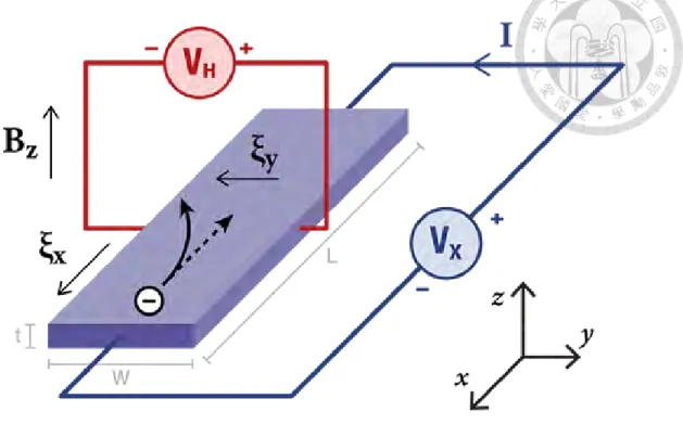
The Hall effect, also called the Ordinary Hall effect (OHE), was first discovered in 1879

by Edwin Hall, from which is derives its name [24]. The Hall effect is the difference in

voltage across a conductor when a current is applied in the presence of an applied magnetic

field (Fig. 2.1). The voltage change across the conductor is due to the Lorentz force acting

upon the charge carriers to be deflected to the edges of the material transverse to the current

flow direction. Since its discovery, several similar phenomenon that lead to accumulation

(17)

of electric charges or spin in material systems have come to share the Hall namesake.

Figure 2.1: Example of the Hall Effect

2.1.1 The Anomalous Hall Effect

Following his discovery of the OHE, Edwin Hall reported the discovery of an effect sim-

ilar to the OHE but of a much larger magnitude in ferromagnetic conductors which was

later named the Anomalous Hall effect (AHE) [25]. After over a century since it was

first discovered, it is now understood that the origins of the AHE can be understood as

a combination intrinsic and extrinsic effects (as shown in Fig. 2.2) [26]. The intrinsic

contribution to the AHE is related to the band structure and its interaction with electric

fields, which were more formally defined through Berry phase and Berry curvature. The

external contribution to the AHE comes from spin dependent scattering of carriers off of

(18)

impurities [2]. The combination of these effects gives rise to the relation:

ρ_xy = R_OH_z+ R_Am_z (2.1)

This equation shows the dependence of the transverse resistance ρ_xy, to the contribution

R_O from the OHE with the application of an external field and also to R_A, a material

specific parameter, and the magnetization in the z direction given by m_z (Fig. 2.3) [2].

Generally the anomalous effect is larger than the ordinary Hall effect contribution. Detec-

tion of the AHE is possible in materials with population differences in carriers or through

injection or excitation of non-equilibrium spin polarized currents [27]. This signal can fur-

ther be used to measure the magnetic orientation of samples with perpendicular magnetic

anisotropy (PMA).

(19)

Figure 2.2: The intrinsic and extrinsic mechanisms giving rise to the AHE [2]

2.1.2 The Spin Hall Effect

Originally proposed by in 1971 by Dyakonov and Perel and then again by Hirsch in 1999,

the Spin Hall effect (SHE) is in many ways analogous to the AHE, but instead of a charge

response, the SHE deals with the spin of the carriers as shown in as seen in Fig. 2.3

[28, 29]. The origins of the Spin Hall effect may come from extrinsic scattering effects as

originally postulated by Dyakonov and Perel or from the intrinsic interaction of spin orbit

coupling in the absence of scattering [3]. Since the first direct observation of the SHE in a

semiconductor by Kato et al. and the subsequent detection of an electrical signal through

the inverse Spin Hall effect (ISHE) by Saitoh et al. the Spin Hall effect has garnered

(20)

significant attention [30, 31].

Figure 2.3: Comparison of the AHE, SHE and ISHE [3]

The interest in the SHE and ISHE lead to a significant number of discoveries when cou-

pled with ferromagnetic samples [3]. Utilizing spin currents generated by spin pumping

allows for measurement of magnetization dynamics. Similarly generation of spin currents

through the SHE can induce spin torques, a key element in the creation of competitive

MRAM devices. The fundamentals of magnetization dynamics and spin torques along

with their importance to MRAM devices are explained in more detail in the next section.

The effects of the SHE are especially apparent in nonmagnetic materials with large

spin-orbit interactions. Application of a charge current through such a material will result

(21)

in a transverse spin current which can be described by:

J_s= ¯h

2eΘ_SH(σ× Je) (2.2)

where J_e is the charge current density, σ is the spin polarization unit vector, Θ_SH is

the spin hall angle and Jsis the spin current density [32].

2.2 Magnetization Dynamics

Understanding magnetization dynamics in the presence of spin torques is of the utmost

importance when designing MRAM devices. Landau and Lifshitz proposed the first equa-

tion governing the motion of precession and damping present in magnetization dynamics

[6]. Excitation of magnetization dynamics through spin transfer torques, first predicted

by Berger [33] and Slonczewski [34] can be added as additional terms to the original

equation proposed by Landau and Lifshitz [4]. Prediction and subsequent experimental

observation of these torques provided a renewed interest in MRAM technologies as spin

torques provided a much more energy efficient way to induce magnetic switching.

2.2.1 The Landau-Lifshitz-Gilbert Equation

An alternative form to the equation Landau and Lifshitz, the Landau-Lifshitz-Gilbert (LLG)

equation describes magnetization dynamics utilizing the Gilbert damping parameter α and

(22)

is the commonly used form of the equation today [35].

d ˆm

dt =−γ0( ˆm× Hef f) + α( ˆm× d ˆm

dt ) (2.3)

Where ˆm is the magnetization, γ₀ is the gyromagnetic ratio and H_{ef f} is the effective

field, which accounts for the contributions from exchange, magnetocrystalline anisotropy,

and the external and self-magnetostatics fields [36]. The first term of the equation is the

precession term, describing the motion of the magnetization around the effective field.

The second term is the damping term, which descibes the rate at which the moment will

align with the effective field (in the case of no external forces). Armed with the LLG,

the magnetization dynamics of specific systems can be found through numerical analysis

utilizing simulations, providing a powerful tool to further validate experimental results.

2.2.2 Spin Transfer Torque

The discussion of the LLG Equation (2.3) above does not account for the spin torques

predicted by Berger [33] and Slonczewski [34]. These spin transfer torques are the result

of a spin current being filtered through two magnetic thin films. The polarized spin current

that flows from the first thin film into the second will tend towards the magnetization of

the second film if its magnetization is not in the same direction as the first film. As the spin

current rotates it passes angular momentum to the magnetic thin film, applying a torque

(23)

[4]. The effects of this torque can be added to the LLG equation resulting in the equation:

d ˆm

dt =−γ0( ˆm× Hef f) + α( ˆm×d ˆm

dt )− γ¯h 2µ₀M_s

1 d

ηJ

e mˆ × ( ˆm_{f ixed}× ˆm) (2.4)

where ˆm and ˆm_{f ixed} are the magnetization unit vectors of the film being acted on

by the torque and the film polarizing the spin current, d is the thickness along the current

direction and M_sis the magnetization [6]. The η^hJ^¯_2e corresponds the efficiency (0 < η < 1)

of the spin transfer torque with the average spin per electron per unit time. The torque

contribution to the LLG equation is also commonly referred to as the (anti) damping-like

torque, as it acts upon the magnetization in the same direction as the damping term [37,

38]. There is also a field-like contribution to the torque, which generally aligns with the

precession term and is proportional to m_{f ixed}ˆ × ˆm. This contribution is generally less

important in switching dynamics and smaller than the damping-like torque by an order or

magnitude or more.

(24)

Figure 2.4: Example of Damping and Torque Vectors [4]

2.2.3 Spin Orbit Torque

Spin-orbit torques can be generated through the Rashba effect, the spin Hall effect and

also through spin-momentum locking in topological insulators (TIs). The Rashba effect

generally is weaker than the SHE and contributes little to SOT induced switching in de-

vices [39]. TIs generally require preserved surface states to generate large SOT which are

difficult to produce using CMOS compatible manufacturing processes. The SHE however

provides a useful means to generate large SOTs to induce switching. As mentioned before,

the SHE will cause a spin accumulation at the edges of a system when a charge current

is applied. The amount of pure spin current generated in the system is given by Equation

2.2. When a material that has a strong SHE, such as 5d transition metals, is placed next to

(25)

a ferromagnetic material, the spin imbalance at the interface will exert a spin orbit torque

(SOT) on the ferromagnetic material (Fig. 2.5). The direction of the torque upon the adja-

cent ferromagnet is determined by σ, the spin polarization unit vector from Equation 2.2.

This method of exerting a torque on the FM has attracted considerable attention as the

spin current that is generated is perpendicular to the charge current, allowing for switch-

ing without having to run a charge current through the MTJ [32, 40]. The magnetization

dynamics of of switching of devices with in-plane anisotropy or PMA can be modeled

using a modified form of the LLG equation given by:

d ˆm

dt =−γ0( ˆm× Hef f) + α( ˆm× d ˆm

dt )− γ¯hΘ_SHJ_{N M}

2eM_st_{N M} mˆ × (ˆσ × ˆm) (2.5)

This equation closely resembles the STT-LLG equation (2.4), with the damping-like

torque contribution being determined by the spin polarization ˆσ and the magnetization of

the free layer ˆm, with M_s being the saturation magnetization and t_{N M} being the thick-

ness of the normal metal. SOT damping-like torques do not directly compete against the

damping term of the LLG [38] and so have a faster switching time than STT. However,

for devices with PMA, SOT current-induced switching requires an applied in-plane field

or some other contribution to break the symmetry allowing deterministic switching to oc-

cur. Similarly in SOT devices there is a smaller field-like torque term which is again

proportional tom_{f ixed}ˆ × ˆm.

(26)

Figure 2.5: SHE generating SOT through a Spin Current [5]

2.3 MRAM Devices

MRAM is a promising non-volatile memory that has, in recent years, become increasingly

common on the market [41]. Despite MRAM’s initial use in the 1980s, it remained in a

niche market position due to several constraining factors that were not solved until more

recently [6]. To be competitive on the market requires balancing of the optimization of

the writeability, readability, and thermal stability while still being easy to integrate with

CMOS technology [5, 20]. As mentioned in the previous sections, the development of

spin torques as a means of switching greatly improved the writeability of MRAM devices.

However this improvement alone was not enough to bring MRAM to market. Two other

significant contributions were the discovery of giant magnetoresistance (GMR) by Fert

(27)

[42] and Grünberg [43] followed by the subsequent discovery of the magnetic tunnel junc-

tions (MTJs) with a large tunneling magnetoresistance (TMR) in Fe/MgO/Fe trilayers

[44, 45, 46]. These discoveries allowed for significant resistance differences between par-

allel and antiparallel states of MTJs (Fig. 2.6), allowing for easily readable devices to be

manufactured [4, 6, 47]. Since then, both academia and industry have spent considerable

resources to develop ever increasingly efficient MRAM devices. In this work, specific

consideration is given to extracting figures of merit from material systems with the aim

developing the next generation of material systems for MRAM devices.

Figure 2.6: Example states of a MTJ [5]

2.3.1 Types of MRAM

There are several types of MRAM designs which can be separated based on their write

methods (Fig. 2.7) [6]. Each type of MRAM possesses their own benefits and drawbacks,

along with particular device physics.

(28)

Figure 2.7: Types of MRAM Devices [6]

Field-driven MRAM

Before the discovery of spin transfer torque, MRAM was limited to devices which used

the oersted field generated by a current in a write line to flip the magnetization as shown

in (a) of Fig. 2.7. These devices suffer from scaleability issues and also the need for large

write currents. Despite these drawbacks, field-driven devices still found applications in

certain fields where the non-volatile nature of these devices was of particular significance.

Spin Transfer Torque MRAM

Following the first demonstration of STT switching [21], STT switching in MTJs [48,

49] and in nanoscale devices [50] proved that it was a viable write function for MRAM

devices. Early versions of STT MRAM had magnetic layers with the anisotropy easy-

(29)

axis lying in-plane [Fig. 2.7 (b)]. In-plane magnetic anisotropy is generally easier to

produce in thin-films due to the competing anisotropy terms and ease with which shape-

anisotropy can be controlled [51, 52]. However, in-plane devices are difficult to scale

below 50 nm while maintaining stability and efficient switching [7, 53]. Realization of a

MTJ with perpendicular anisotropy (PMA) which maintained high thermal stability, low-

current switching and a large MTJ ration by Ikeda et al [54] was a major step to scaling

STT MRAM devices below 50 nm. STT MRAM still suffers from the drawback of having

both the read and write voltages cross the MTJ barrier. In cases where the voltages are

high, they may lead to breakdown of the MTJ and device failure [6].

Three Terminal MRAM

A solution to the issue of sending a write voltage across the MTJ barrier is use of spin

orbit torques in a three-terminal device to either cause domain wall motion or switching

of a free layer (Fig. 2.7). Demonstrations of devices utilizing switching of a FM layer

were first done by Miron et al. [55] and Liu et al. [56]. Subsequent proposals for three-

terminal devices showed potential to improve reliability for MRAM devices [32, 40]. The

design for these three-terminal devices is simple: a write line, consisting normally of a

heavy metal (due to its large spin orbit coupling) lies on the free layer side of a MTJ

(generally CoFeB/MgO/CoFeB) which is connected to a read channel (Fig. 2.8). A write

current can be passed through the write line generating a transverse spin current to flip

(30)

the free layer of the MTJ. Reading the device only requires running a current through

the MTJ. The benefits of utilizing SOT MRAM devices with PMA are similar to those

of STT MRAM, i.e. better scalability and stability, but with the additional benefit that

the write current doesn’t not need to flow through the MTJ which also improves write

times [57]. However the drawback of SOT switching in PMA layers is that an additional

contribution, normally in the form of an applied field, is necessary to break the symmetry

for deterministic switching to occur [56, 58]. Furthermore, the strength of the torques

generated by the SHE is a material dependent property that is proportional to the charge

current and so is limited by the intrinsic properties of the system. Research into improved

material systems that produce a large spin current and systems that allow for deterministic

switching without the need to apply an external field are ongoing.

Figure 2.8: Example of a three-terminal SOT MRAM device [5]

(31)

2.3.2 Figures of Merit

When characterizing and engineering material systems to design optimal MRAM devices,

there are several figures of merit. The measurement and data analysis programs in this

work are designed to extract values as quickly and accurately as possible. The physical

background and use of each of these values is explained in detail.

Critical Field

The value at which an external field causes switching in a device. In the measurements

presented in this work, this value varies with applied current and applied in-plane field,

as heating and alignment of magnetic moments both influence the energy necessary to

change the magnetization of a layer from one orientation to another [18, 58].

Thermal Stability

For all MRAM devices, the energy of a two state system (parallel and anti-parallel) can be

thought of as two equilibrium states separated by an energy barrier (Fig. 2.9). The height

of this energy barrier E_bis the value that must be overcome for a switching event to occur.

The thermal stability of a device is the ratio of this energy barrier and the operational

temperature as shown in Equation 2.6 [59].

∆ = E_b

kbT (2.6)

(32)

Figure 2.9: Energy barrier between parallel and anti-parallel states [7]

The thermal stability of a device determines the memory retention failure in standby

mode [6]. As the number of devices increase, the thermal stability factor must also in-

crease to ensure that the number of failures over 10 years stays below the acceptable toler-

ance. One of the main reasons devices with PMA are preferable to devices with in-plane

anisotropy is the origins of anisotropy, which directly corresponds to the height of the

energy barrier [6]. The stability factor of circular PMA devices where switching is gov-

erned by the macrospin model (typically dimensions of less than 30 nm) is given by the

following equation:

∆ = E_b

kbT = [(K_v− (1/4)µ0(3N_z− 1)Ms²)t + K_s]^π₄w²

kbT (2.7)

(33)

where the K_vand K_sare the bulk and interfacial anisotropy energy terms. For CoFeB/

MgO interfaces, PMA generally comes from interfacial effects. The height of this energy

barrier, it is possible to calculate the mean time between flipping events over this energy

barrier is given by the Néel-Brown theory of relaxation [6] given by the equation:

τ_N = τ₀exp KV

k_BT (2.8)

where τ₀ is the attempt time, (generally 1 ns), and KV is the height of the energy

barrier, which is determined by the magnetic anisotropy energy density and the volume as

seen in Equation 2.7.

For large devices, switching is no longer coherent but instead driven by domain wall

nucleation and subsequent motion. The energy barrier for domain wall nucleation can be

significantly lower than that given by the macrospin model. In the case where domain

wall nucleation and motion dominates, the energy barrier can be estimated by using the

energy of a domain wall which is given by the following formula [59, 60]:

∆ = 4wt√

AexHk(MS/2)

k_bT (2.9)

where H_kis the anisotropy field, M_S is the saturation magnetization, wt is the width

and thickness and A_exis the exchange length.

(34)

Critical Current

Critical current, also known as the switching current I_cis the minimum necessary current

required for switching the magnetization of device. This value is of key importance in

MRAM devices as it will determine the power consumption of the device. It is standard

to refer to the corresponding current density Jcwhich is area independent, allowing more

convenient comparison between different devices regardless of size. The most general

case for the zero-thermal-fluctuation critical current is given by [60]:

J_c0 = 2e

¯

hµ₀M_Stα(H_c+ M_{ef f}/2)

J_s/J_e (2.10)

where H_c is the coercive field of the FM layer, M_{ef f} is the effective demagnetizing

field and α is the damping constant. For devices with PMA, generally the effective de-

magnetizing field is much smaller than that of the coercive field and can be ignored. Fur-

thermore, in the case of SOT switching, the torque direction does not compete with the

damping and so is independent of the damping constant [38]. Upon extracting the critical

current, it is possible to calculate the thermal stability based upon the Néel-Brown equa-

tion (2.8) where the thermally-activated critical current J_cis less than the critical current

at zero temperature, also known as the zero-thermal-fluctuation critical current, J_c0[61]

(35)

as shown in the following equation:

J_C = J_C0[1− 1

∆₀ lnt_p

τ₀] (2.11)

In order to extract both the thermal stability and the zero-thermal-fluctuation critical

current from this equation, measurements can be run over a range of varying pulse widths.

For different pulse widths there are two regimes, a thermally activated regime, where ther-

mal fluctuations aid switching and a regime where thermal effects are minimal, requiring

large current to generate strong enough torques to induce switching. The details of this

process are explained in further detail in Chapters 4 and 5.

Spin Hall Angle and Torque Efficiencies

The Spin Hall Angle Θ_SH is a material dependent term that shows how much charge

current is converted into spin current in a given system. Materials that have large spin

hall angles are of particular interest to MRAM applications, as a larger angle means lower

power consumption. The origins of the spin Hall angle in material systems can come

from the SHE (large spin-orbit interactions) or from the intrinsic band structure of the

material, such as the Rashba effect from dissimilar interfaces or spin-momentum locking

in topological insulators and some 2D material systems. For SOT-MRAM devices, heavy

metals (HM), such as W, Ta, Pt, with stronger spin orbit coupling, leading to larger spin

(36)

Hall angles. The spin Hall angle is commonly defined as:

Θ_SH = 2e

¯ h

|Js|

|Je| (2.12)

However, when measuring the spin Hall angle of a material system it is important to

also consider interfacial effects, which tend to reduce the interfacial spin transparency and

thereby reduces the effective spin Hall angle [37]. This transparency is determined by

primarily by the spin-mixing conductance and yields:

Θ_SH = ξ_DL

(2G^↑↓_{ef f}/G_{N M}) = ξ_DL

T_int (2.13)

where ξ_DLis the damping-like SOT efficiency, G^↑↓_{ef f} is the effective spin mixing con-

ductance, G_{N M}is the spin conductance of the normal metal and T_intis the interfacial spin

transparency [37]. Measurements of the spin Hall angle for a system are quite sensitive to

the transparency term which is based not on a single material but on the interface of the

two materials. Due to this and the choice of measurement technique, comparison of SHA

of a material across multiple systems can result in a wide range of values (shown in Fig.

2.10) [62]).

(37)

Figure 2.10: Spin Hall ratio measurements. Measurements of spin Hall angles values should be constant for a given material [8, 9, 10, 11, 12, 13, 14, 15, 16, 17]

An easier and more clear approach to classifying SOTs that allows for comparison

across different material systems is through measuring the damping-like SOT efficiency

ξDL from Equation 2.13. This efficiency in multidomain systems with PMA is given by

the equation:

ξ_DL = 2e

¯ h(2

π)µ₀M_st^{ef f}_{F M}(H_z^{ef f}

J_e ) (2.14)

where H_z^{ef f} is the effective field generated by the applied current Je [18, 63]. For

devices with in-plane anisotropy, the damping-like SOT efficiency can be written as:

ξ_DL = 2e

¯

hµ₀M_st^{ef f}_{F M}α(H_c+M_{ef f}

2 )/J_c0 (2.15)

(38)

where M_{ef f} is the effective demagnetization field and J_c0is the threshold critical cur-

rent density [19, 63].

(39)

Chapter 3 Measurement Systems

Measurements in our lab can be broken into two groups, electrical and optical. Each probe

station is capable of doing real-time optical (MOKE) measurements and also real-time

electrical measurements. As probe stations are added for increasingly specific purposes,

a universal system of calibrating instruments, running measurements and data collection

is important for maintaining consistency in measurements and speed and flexibility in the

measurement process. This section outlines the framework from which the measurement

programs are built.

3.1 Machine Configuration

Currently our lab has two probe stations, with several additional stations still being set up.

The first probe station consists of an in-pane and out-of-plane electromagnet, both with

(40)

their own power supply, a DSP 7265 Signal Recovery Lockin-amplifier and a Keithley

2400 sourcemeter and Keithley 2000 multimeter and a Lakeshore 475 Gaussmeter. The

second probe station has the same machines but the in-plane and out-of-plane electromag-

nets are separated. Both stations have a optical microscope for MOKE measurements and

to ensure proper contact is made between the probes and the electrodes. Diagrams of a

probe station setup are provided in the figure below. The Gaussmeter probe and optical

microscope are stationed above the location marked (a) where the sample is placed upon

a stage. The arrows from (b) mark the locations of the electromagnets.

Figure 3.1: Example Probe Station

3.2 Programming Environment

All programs in our lab are run using Python 3. The instruments used for measurements

are connected either using GPIB or USB connections. Communications with the devices

are run utilizing the PyVISA [64] front-end to the National Instruments’ VISA library

(41)

[65]. The specific versions of the packages used are listed in the table below.

Table 3.1: Packages Used

Package Version

pillow 6.0.0

pandas 0.24.2

pymeasure 0.7

numpy 1.16.4

pyvisa 1.9.1

pyvisa-py 0.3.1

tkinter 8.6.8

jupyterlab 0.35.4

conda 4.7.12

python 3.7.3

mss 4.0.2

3.3 Device Fabrication

Samples in our lab are generally deposited in a high vacuum sputtering chamber using

magnetron sputtering. Devices are patterned using photolithography and/or etching using

ion-beam milling. The Hall-bar devices used to perform the majority of the measurements

(42)

described in this work are micron-sized, with lateral dimensions of either 5 or 10µm×

60µm [w in Fig 3.2 (a)]. In this work, the current channel of the Hall Bar device will be the

x direction, with the cross bars lying in the y direction and the z direction corresponding to

the direction normal to the surface of the bar, as shown in (b) of the figure below. Voltage

measurements are made via the cross bars, perpendicular to the current channel of the

device.

Figure 3.2: (a) Hall bar image with probes in contact with electrodes. (b) Schematic of Hall bar and an example stack structure

(43)

Chapter 4 Measurement Programs

Redesign of the measurement programs used in the lab was done with several specific

goals. The first was to build a universal formatting for measurement scripts so that scripts

would be both easy to program and easy to read. The second goal was to standardize ver-

sion control across the current probe stations, and allow for new stations to be easily added

in as necessary. The third goal was to have built in error functions to make troubleshooting

easier and to protect vulnerable lab equipment. The final goal was to ensure that future

updates would apply to all scripts, allowing system wide updates to be done with ease as

necessary.

(44)

4.1 Program Structure

As opposed to previous versions of measurement scripts used in the lab, this new version

is comprised of several classes which are imported in specific measurement scripts. To run

a measurement, a script needs to create an instance of the GUIBaseClass which provides

the UI framework for the measurement parameters along with a graph, progress bar, dis-

play box for messages, and buttons which control the measurement. The measure button

spawns a child process which runs the measurement and manages tasks necessary for all

measurements. The child process can be paused or terminated at any time with no risk to

the instruments currently in use and no major delay to the user.

4.1.1 UI Base Structure

UI programming requires a large number of lines of code to create a functional interface.

The overall UI structure for measurements run in our lab varies only minimally with dif-

ferent text and measurement loop parameter settings (shown in Fig. 4.2). In an effort to

remove lengthy sections of repetitive code from individual measurements, I built a univer-

sal UI backend. The interface consists of five sections: a graph, a progress bar, a display

box, a buttons section and the loop parameters. The graph is run using animation from the

Python matplotlib package. Animation automatically handles blitting along with running

on a separate timer which keeps the GUI event loop from repeatedly blocking. Blitting

(45)

is the process by which the animation function saves and reuses previous data allowing

only a small section of the graph to be re-rendered each time. Utilization of the animation

function alone greatly increases rendering speed and can speed the measurement of a data

point by up to several seconds, depending on the number of data points (Fig. 4.1). The

progress bar and display box update as the measurement process runs, with the progress

bar estimating the time left until completion and the display box printing any important

messages to the user.

Figure 4.1: Run time comparison of new code (Multiprocessing) vs. old code (Threading with out animation)

Errors that occur when attempting to run the measurement process should be caught

and displayed in the display box, making it easier for the user to debug. The buttons sec-

tion generates five separate buttons: output, change directory, measure, stop and quit (Fig.

4.2). Change directory allows the user to change to a specific directory instead of the de-

fault measurements directory. Output creates a top level window which allows the user to

(46)

run a single pulse output field at a given strength for a given duration. It will automatically

detect the available output directions available and allow the user to determine the output

direction if there is more than one direction available. The measure button spawns the

child process and begins a measurement. Running multiprocessing instead of multithread-

ing also improves the measurement speed, with average measurement times for a single

data point being around 0.09 seconds for multithreading and only 0.002 seconds for mul-

tiprocessing. The stop button will pause a currently running measurement and allow the

user to continue at any time or to safely terminate the current measurement without exiting

the program. The quit button safely terminates any measurement currently running and

then exits the program. The loop parameters are user defined in the measurement script.

This flexibility allows each script to have its own labels for each entry, along with default

values specific to the measurement.

(47)

Figure 4.2: Graphical User Interface for Measurements (a) The graph region, (b) the progress bar, (c) the display box, (d) the loop parameters and (e) the buttons

4.1.2 Measurement Structure

In order to standardize universal functions for all measurements, the measurement class

is built to run three nested for loops with functions defined by the specific measurement

script. Through this process, the measurement class will automatically handle the follow-

ing:

• Creation of loop array values

Arrays are built using the numpy arange(start, stop, step) function, with the start,

stop and step being user designated values from the UI. The user can also choose

(48)

loops running from low to high and back to low, zero to high to zero to low and

back to zero or from high to low to high for the x values of the measurement. This

offers great flexibility for the user, measurements to be in specific ranges with any

step size. Should the user only want to use a single value, choosing a step size of

zero will return an array with just the corresponding stop value.

• Initializing and shutting down instruments

To ensure that communications with any active resources is properly handled, the

measurement class will automatically handle creating an instance of each instrument

along with calling shutdown on that instance when the measurement is either fin-

ished or interrupted. Proper resource management ensures that GPIB bus has been

flushed of data.

• Managing pause and quit flags

Before each measurement of corresponding to an x data point, the measurement

class will check whether the quit flag is set. If set, the program will break the for

loops and run the shutdown procedure before informing the user that the shutdown

is complete. For every value in the second for loop, the measure class checks if

pause has been flagged. If so, it will pause the program until the user chooses to

continue.

• Updating UI graph and progress parameters

(49)

The graph and progress bar are both updated through the GUIBaseClass, which

is the parent process. Communication with the parent process happens through a

queue, which handles updating graph titles, updating the progress bar and printing

any messages to the user in the UI display box. The x and y data is stored in a shared

array and so the GUIBaseClass can automatically access it, minimizing the amount

of data being sent through the queue.

• Delay calibration and amp protection

To prevent damage to the electromagnet power supplies, the measurement class au-

tomatically checks if a field will be applied for a given for loop. If the maximum

value of that loop exceeds the given power supplies maximum voltage, then an error

is displayed to the user and the measurement quits. Furthermore, delay calibrations

have been added which ensure that the electromagnet has reached the desired mag-

netic field before the measurement continues. Both the calibration factor and the

protection voltage are stored as universal values and are easily updated.

• Saving Data

Data is saved to comma separated values (csv) files using universal formatting. The

file will include columns for the x and y values, along with an additional column for

extra measurements, i.e. Gaussmeter field readings. Furthermore there are columns

corresponding to each fixed value, the type of measurement, loop direction, sample

(50)

name and the time the data was saved. The reason for this formatting is explained

in further detail in the Analysis Programs section.

The measurement class also has the added ability of handling wide-field MOKE mea-

surements [66] through a top level window that allows the user to select the portion of the

monitor they wish to measure.

4.1.3 Command Script Structure

Measurements can be quickly scripted to meet user requirements by defining the three

functions (Fig. 4.3) that the measurement class will run. These functions are controlled

by keyword arguments that are set through the UI. Utilizing these keyword arguments, it is

easy to give command resources to perform any number of tasks. For users who are less fa-

miliar with programming languages and resource control, the use of pymeasure [67] offers

a mature documentation making programming resources trivial. Each function is passed

an output argument corresponding to the current array value from the measurement class,

a delay time determined by the measurement class, a dictionary of resources with keys that

are set by the user and values corresponding to the individual instances. Any additional

dictionary parameters set by the user are passed in through a dictionary. Resources can be

initialized to measurement specific settings utilizing the index value that is passed to the

function fix_param1. In cases where measurements need to reference the current output

values from the first two nested loops, the measure_y function is also passed those two

(51)

values.

Figure 4.3: Functions for AHE measurements

To ensure that graphs and saved data have the appropriate titles and units for a given

measurement, the graph_dict values can be changed to any string. The resources used by

the measurement are defined in a separate dictionary, which can either use the specific

address of the machine or can import the address from the FieldControls script ( see Ap-

pendix). For each script, any number of dictionaries can be passed to the instance of the

GUIBaseClass to define the loop parameters and any other variables needed. The Mea-

surementClass uses the loop_commands dictionary to import not only the functions, but

also to define which variables to use as the start, step and stop of each array. As shown

in the figure below, the loop_commands for each loop (fix1, fix2, x) correspond to the

dictionary items of one of the command dictionaries.

(52)

Figure 4.4: Dictionaries for AHE measurements

4.1.4 Universal Settings

Perhaps one of the most time consuming yet overlooked features of running programs

across multiple systems is version control. For probe stations, changes to how resources

are connected, updates to equipment, and a large number of users can quickly result in

multiple versions of code. To remove the need for users to save individual scripts default

settings, system specific settings have now been moved to a single file. This file (Field-

Controls.py) also stores electromagnet specific features such as the conversion factor (Oe/

V) and the maximum voltage output. For each station, the GPIB addresses of individual

resources are also stored. Measurements will automatically import the appropriate values

for a station based on the user name from that station.

(53)

4.2 Accuracy Improvements

To improve the accuracy of measurements, calibration of electromagnets’ conversion fac-

tor and delay times have been automated. By cycling through the voltage outputs of a given

power supply and measuring the corresponding outputs, a simple linear fitting yields an

accurate conversion factor that can be used. To ensure that measurements are taken at

the desired field strength, delay time fitting can be done. For a given number of voltage

steps, the script will measure the change in electric field and the time it takes to reach

saturation at said voltage. From this, a fitting can be done so that for any field step size

the measurement program will delay for the appropriate amount of time.

4.3 Measurement Scripts

In this section, specific scripts for three types of measurements are explained in detail.

The results of these measurements are analyzed using the data analysis notebooks which

are explained in further detail in the next chapter. For the full code of these scripts, along

with other scripts used in our lab reference to the Appendix of this work.

4.3.1 AHE Measurement

To find the damping-like SOT efficiency (Equation 2.14) for devices with PMA, hystere-

sis loop-shift measurements by measuring the change in resistance from the AHE while

(54)

sweeping an out-of-plane field at various fixed in-plane field and current strengths. As

shown in Fig. 4.4, the GPIB addresses for this program are imported using default settings

from FieldControls. Magnetic fields are applied using a voltage from the Signal Recovery

DSP 7265 Lockin Amplifier, a Keithley 2400 sourcemeter is used to apply a DC current

across the current channel of the device 3.2, a Keithley 2000 sourcemeter is used to mea-

sure the voltage across one of the cross bars and a Lakeshore 475 Gaussmeter is used to

measure the accuracy of the in-plane applied field. The magnetic field values and current

values are defined in the control dictionaries (Fig. 4.4). Each measurement will consist of

scanning over the given x values defined by the start, stop, step and the loop direction as

explained in the previous section. In the first iteration of the first for loop, Keithley 2000

is set to measure voltage using the auto range mode and Keithley 2400 is set to apply a cur-

rent using the auto range source function. The Lockin Amplifier is then set each iteration

of the first for loop to output a voltage corresponding to the specified H_x output (Oe) by

taking the output value and dividing by the appropriate conversion factor. The program

then sleeps for a time specified by the step size in field output (Fig. 4.3, fix_param1).

For each iteration of the first for loop, the measurement will iterate through all values in

the second for loop. For AHE measurements, this corresponds to commanding Kiethley

2400 to output a DC source milliamp current (Fig. 4.3, fix_param2). For each iteration

of the second for loop, one entire measurement cycle is done. This corresponds to calling

measure_y for each x value in the final for loop (Fig. 4.3). Similar to fix_param1, the

(55)

Lockin is commanded to output a voltage to set an applied field in the z direction. After

a delay, the gaussmeter takes a measurement of the in-plane field and Keithley 2000 will

take i voltage measurements, where i is the number of averages selected by the user. The

resulting averaged voltage is divided by the DC current output (in Amps) to get the resis-

tance. The H_z value (Oe), resistance value (Ohms) and the reading from the gaussmeter

(Oe) are returned to be saved. Choosing Hx to equal 2500 with no step, and current start

to be -6, current stop = 6 and a step size of 12, and hz start = -1000, hz stop = 1000, and

the loop direction to be low-high, we can obtain hystersis loops similar to those shown in

the figure below.

Figure 4.5: Representative Data from AHE Measurements [18]

(56)

4.3.2 AMR Measurement

For devices with in-plane magnetic anisotropy, AMR measurements can be done to find

the damping-like SOT efficiency. The script for AMR measurements is identical to the

AHE measurement with the exception of the direction of the applied fields. These changes

correspond to changing the loop_commands’ key value pairs to hz start, stop and step for

the fix1 keys and the hx for x start stop and step keys. Updates to the graph title and

fixed values are done to ensure that data is saved properly and the UI displays the proper

information. For AMR measurements, there is generally no need to apply an out-of-plane

field, and so the hz default values are set to 0. Using a low-high measurement loop at two

current values will result in graphs similar to those shown in the figure below.

Figure 4.6: Representative Data from AMR Measurements [19]

(57)

4.3.3 Pulse Switching Measurement

Current-induced switching measurements can be used to find the threshold critical cur-

rent and thermal stability in devices regardless of their magnetic anisotropy. For devices

with in-plane magnetic anisotropy, the threshold critical current is also necessary to cal-

culate the damping-like SOT efficiency, as shown by Equation 2.15. Current-switching

measurements are done by varying a pulse width at given applied in-plane field values

and measuring the resistance after applying current pulses. Similar to the scripts above,

controls are set for current and applied fields, along with imported default settings of in-

strument GPIB addresses, conversion factors and DAC outputs. This script uses the same

instruments as the AHE and AMR scripts, the only difference being the Keithley 2400

sourcemeter is used to apply current pulses for writing and reading. The fix_param1 func-

tion is identical to that of AHE, with instruments being set to the proper settings the first

time and a H_x field being output via the Lockin Amplifier. For fix_param2, the function

only passes, as the output value passed to fix_param2 corresponds to the pulse width. To

take pulse measurements for a given pulse current strength, the function measure_y has

several steps [Fig. 4.7 (a)]: First, the applied in-plane field strength is measured by the

gaussmeter. Following this measurement, the sourcemeter applies a milliamp pulse for

the pulse width duration. A slight write-read delay can be chosen by the user, creating

discrete write and read pulses. The sourcemeter is then used to apply the user defined

(58)

sensing current, which is applied for the number of seconds set by the read pulse width

value before Keithley 2000 is used to average a number of voltage readings, similar to the

AMR and AHE scripts. The function then returns the current pulse (mA), the measured

resistance (Ohms) and the measured in-plane field (Oe).

Figure 4.7: (a) Measure_y function for pulse switching script, (b) Representative pulse switching data of a sample with in-plane magnetization

(59)

Chapter 5 Analysis Programs

Analyzing data can be a slow and time consuming process if the data is not properly or-

ganized [68]. One way to minimize the time spent on analysis is to organize data into

tidy datasets, defined by Wickham [69] as a dataset “where each variable is a column and

each observation is a row and each type of observational unit forms a table”. Previously,

data from our measurement programs was quite messy [see Fig. 5.1 (a)], and lacked a

universal formatting. This made the process for tidying data sets slow and error-prone.

The new measurement programs from the previous section automatically save data in a

tidy format [Fig. 5.1 (b)]. For messy datasets from previous results, there are several

scripts I developed that allow user who is unfamiliar with programming to tidy the data.

Tidied data allows users to quickly perform analysis through the notebooks introduced in

this section, which speeds up the extraction of figures of merit. Second, the tidied data is

(60)

organized in such a way that users can quickly perform comparisons on larger data sets

over any range of variables. The notebooks here are built so that users who are unfamiliar

with programming can quickly extract the information they need, without having to worry

about errors, allowing them to focus on the meaning of the results. Users who are more

familiar with programming can utilize the flexibility of notebooks and run comparisons

and analysis on the datasets.

Figure 5.1: Example Datasets: (a) Previously stored messy dataset, note variables not stored as columns. (b) Tidy dataset, note that each variable is a column

5.1 Pre-processing of Data

Despite the datasets being tidy, the actual results from measurements may be messy. Mea-

surement readings may have outliers due to imperfect contact between the probe and the

device, entire measurement loops that need to be ignored due to the device burning, or

vibrations causing the results to be unusable. To speed up the process of weeding out un-

desirable measurements from the good ones, I built several ways to ignore data into the

analysis notebooks. The first method allows the user to manually select specific datasets

to ignore based on visual inspection (Fig. 5.2). All imported data is graphed, so that the

user can quickly check if the measurement loops imported. The graphical output can ei-

(61)

ther be raw data or normalized data, as in some cases comparing the raw data can obscure

the individual data sets, as shown in Fig. 5.3. Subsequent methods to ignore datasets are

based upon automated error catching processes which is explained in further detail in the

next section. For datasets where potential errors are detected the user is given the option

to ignore the data from any subsequent analysis and final results.

Figure 5.2: Notebook cell with user input ignore data (left) and the graph output of the ignored data set (right)

Figure 5.3: Example of graphed datasets from AMR measurements

透過Python進行磁性薄膜量測及數據分析

National Taiwan University Master Thesis

Acknowledgements

要

Abstract

Contents

List of Tables

List of Figures

Chapter 1

Introduction

1.1 Motivation

Chapter 2

Theory

2.1 Hall Effects

2.1.1 The Anomalous Hall Effect

2.1.2 The Spin Hall Effect

2.2 Magnetization Dynamics

2.2.1 The Landau-Lifshitz-Gilbert Equation

2.2.2 Spin Transfer Torque

2.2.3 Spin Orbit Torque

2.3 MRAM Devices

2.3.1 Types of MRAM

2.3.2 Figures of Merit

Chapter 3

Measurement Systems

3.1 Machine Configuration

3.2 Programming Environment

3.3 Device Fabrication

Chapter 4

Measurement Programs

4.1 Program Structure

4.1.1 UI Base Structure

4.1.2 Measurement Structure

4.1.3 Command Script Structure

4.1.4 Universal Settings

4.2 Accuracy Improvements

4.3 Measurement Scripts

4.3.1 AHE Measurement

4.3.2 AMR Measurement

4.3.3 Pulse Switching Measurement

Chapter 5

Analysis Programs

5.1 Pre-processing of Data