Proceedings of the ASME 2017 36th International Conference on Ocean, Offshore and Arctic Engineering OMAE2017 June 25-30, 2017, Trondheim, Norway
OMAE2017-61747
CALIBRATION OF LONG-TERM TIME-DOMAIN LOAD GENERATION FOR FATIGUE LIFE ASSESSMENT OF OFFSHORE WIND TURBINE
Bryan Nelson CR Classification Society
Taipei, Taiwan
Yann Quéméner CR Classification Society
Taipei, Taiwan
Tsung-Yueh Lin CR Classification Society
Taipei, Taiwan
Hsin-Haou Huang
Department of Engineering Science and Ocean Engineering, National Taiwan University
Taipei, Taiwan
Chi-Yu Chien
Department of Engineering Science and Ocean Engineering, National Taiwan University
Taipei, Taiwan
ABSTRACT
This study evaluated, by time-domain simulations, the fatigue life of the jacket support structure of a 3.6 MW wind turbine operating in Fuhai Offshore Wind Farm. The long-term statistical environment was based on a preliminary site survey that served as the basis for a convergence study for an accurate fatigue life evaluation. The wave loads were determined by the Morison equation, executed via the in-house HydroCRest code, and the wind loads on the wind turbine rotor were calculated by an unsteady BEM method. A Finite Element model of the wind turbine was built using Beam elements. However, to reduce the time of computation, the hot spot stress evaluation combined FE-derived Closed-Form expressions of the nominal stresses at the tubular joints and stress concentration factors. Finally, the fatigue damage was assessed using the Rainflow Counting scheme and appropriate SN curves. Based on a preliminary sensitivity study of the fatigue damage prediction, an optimal load setting of 60-min short-term environmental conditions with one-second time steps was selected. After analysis, a sufficient fatigue strength was identified, but further calculations involving more extensive long-term data measurements are required in order to confirm these results.
Finally, this study highlighted the sensitivity of the fatigue life to the degree of fluctuation (standard deviation) of the wind loads, as opposed to the mean wind loads, as well as the importance of appropriately orienting the jacket foundations according to prevailing wind and wave conditions.
NOMENCLATURE CF Closed-form D Fatigue damage
U Standard deviation of wind speed
nom Nominal stress
INTRODUCTION
Taiwan has recently started to evaluate the potential for offshore wind energy production off its west coast, which was selected by 4C Offshore Limited as one of the world's best wind locations [1], having considerable development potential due to high wind energy, stable wind speed, and shallow water depth.
The authors [2, 3] previously showed that typhoon conditions are crucial design problems for the ultimate strength of the unit. However, fatigue strength can be just as significant, especially at the tubular joint connections of the jacket support structure, which are subjected to numerous load cycles during the 20 years of design life. To this end, the authors [4] recently conducted time-domain simulations to reproduce the long-term evolution of the wind and wave loads on the unit and to evaluate the corresponding structural response. This was done by collating joint probability tables to produce a covariance matrix for the considered environmental load parameters, namely wave height, wave period, and wind speed, and then stochastically generating the desired 20 years of weather states through Cholesky decomposition of said covariance matrix.
While this recent study was highly beneficial in validating the adopted Finite Element-derived Closed Form (CF) approach and demonstrating the low damage inflicted upon the jacket foundation‟s X-joints, a lack of sufficiently detailed environmental data led the authors to implement the present study, which seeks to provide a more accurate fatigue life assessment, while further reducing computation times. This fatigue life assessment is based on the probabilities of occurrence of each combination of environmental parameters, taken directly from a set of decomposed joint probability tables.
Due to the long computation times of time-domain simulations, the present study adopted the same wave load
generation model and CF structural response approach that were previously [4] shown to produce a good trade-off between time-efficiency and simulation accuracy. A more accurate wind generation model was also adopted. The calculations were conducted according to DNVGL Guidelines [5], in compliance with the IEC‟s 61400-1 International Standard [6].
The long-term environmental conditions are described in the second section of this paper, and the short-term conditions, based on IEC and DNV guidelines, and the numerical models employed to calculate the wind and hydrodynamic loads, are described in the third and fourth parts. The fifth part of this paper presents the hot spot stress evaluation approach that combined FE-derived Closed-Form expressions of the nominal stresses at the tubular joints and stress concentration factors.
Finally, the fatigue damage was assessed using the Rainflow Cycle Counting scheme. The fatigue life assessment results and suggestions for future improvements are discussed in the Conclusions.
LONG-TERM STATISTICAL REPRESENTATION OF ENVIRONMENTAL CONDITIONS
The long-term statistical environment was based on a preliminary site survey gathered over three years. In this survey, six scatter diagrams, showing the number of one-hour observations of each significant wave height and peak wave period (Hs-Tp), were presented for a range of hub height wind speeds Uhub. Joint probability tables for wind speed, wind direction, wave height, wave period, and wave direction were analysed, and, based on a strong correlation between wind speed and wave height, i.e. corr(Uhub, Hs) = 0.72, and high similitude between component joint-probability distributions for wind direction wnd, each of the six Hs-Tp-Uhub tables were further decomposed into twelve component tables, one per wind direction. In this way, the probability of occurrence of each combination of environmental parameters could be easily referenced from 72 Hs-Tp-Uhub-wnd joint probability tables, with a total of 120 Hs-Tp probabilities per table × 72 tables, giving 8640 environmental load combinations.
Finally, the contribution of each short-term condition to the total fatigue life was weighted by its frequency of occurrence, such that the fatigue damage was mostly driven by frequently occurring mild wind and wave conditions, as opposed to extreme conditions, such as typhoons, which occur far more seldom, and therefore represent only a small part of the total fatigue life of the structure.
SHORT-TERM TIME DOMAIN WAVE LOADS
For each sea state, the selected JONSWAP sea spectrum [7]
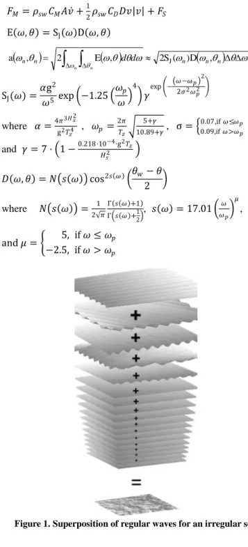
and directional spreading function were applied to obtain an irregular, time-varying flow field. The consequent wave loads were determined by the Morison equation, expressed in Eq. (1), executed via the in-house HydroCRest code. The determination of coefficients followed DNVGL Guideline [5], where the slamming term Fs is neglected in normal wave conditions.
Based on the superposition solution of potential flow theory, an irregular sea surface can be decomposed into an
infinite number of regular component waves, which are formulated by amplitude, direction, frequency, and phase, as shown in Fig. 1 [8]. For a given power spectrum, such as directional JONSWAP, Eq. (2), the amplitude is calculated by Eq. (3). The JONSWAP formula is expressed by Eq. (4), and the directional spreading function is the cosine-power equation, Eq. (5). A GPU accelerator was utilized [9] to speed up the wave load simulation by parallel processing the thousands of component waves and element nodes and then performing a sum reduction of each line load to an overall overturning moment to comply with the close-form formulation of FEA.
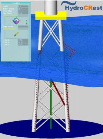
Figure 2 shows the nodal forces and total force in HydroCRest.
𝐹𝑀= 𝜌𝑠𝑤𝐶𝑀𝐴𝑣 +12𝜌𝑠𝑤𝐶𝐷𝐷𝑣 𝑣 + 𝐹𝑆 (1)
E 𝜔, 𝜃 = SJ 𝜔 D 𝜔, 𝜃 (2)
n n nn n
n n
d
d 2S( )D , ,
E 2
,
a J (3)
SJ(𝜔) =𝛼g2
𝜔5 exp −1.25 𝜔𝑝
𝜔
4 𝛾exp −
𝜔 −𝜔𝑝 2
2𝜍2𝜔𝑝2 (4)
where 𝛼 =4𝜋g23𝐻𝑠2𝑇
𝑧4 , 𝜔𝑝 =2𝜋𝑇
𝑧 5+𝛾
10.89+𝛾, σ = 0.07,if 𝜔≤𝜔𝑝 0.09,if 𝜔>𝜔𝑝 , and 𝛾 = 7 ⋅ 1 −0.218⋅10𝐻−4⋅g2𝑇𝑧
𝑠2
𝐷 𝜔, 𝜃 = 𝑁 𝑠 𝜔 cos2𝑠 𝜔 𝜃𝑤− 𝜃
2 (5)
where 𝑁 𝑠 𝜔 =2 𝜋1 Γ 𝑠 𝜔 +1
Γ 𝑠 𝜔 +12 , 𝑠 𝜔 = 17.01 𝜔𝜔
𝑝 𝜇
,
and 𝜇 = 5, if 𝜔 ≤ 𝜔𝑝
−2.5, if 𝜔 > 𝜔𝑝
Figure 1. Superposition of regular waves for an irregular sea
Figure 2. Nodal load distribution on members (thin lines) and total load on center of force (thick lines) in irregular sea
SHORT-TERM TIME DOMAIN WIND LOADS
The concept of wind turbulence is explained in DNV [5] as
“the natural variability of the wind speed about the mean wind speed U10 in a 10-minute period” for which “the short-term probability distribution for the instantaneous wind speed U can be assumed to be a normal distribution” with standard deviation
U. In the present study, the short term wind states were modeled on the IEC 61400-1 Normal Turbulence Model (NTM) [6], with a reference turbulence intensity of Iref = 0.16, as per the requirement of the Taiwanese Ministry of Economic Affairs [10] that the pilot wind turbine to be installed in the Fuhai Offshore Wind Farm must be IEC 61400-1 Class IA compliant. Following the NTM, the standard deviation σU of the wind speed for a given U10 is calculated by Eq. (6):
σU = 𝐼𝑟𝑒𝑓(0.75 𝑈10+ 3.8) (6)
In order to generate a more realistic short-term wind state, the wind speed fluctuations were calibrated against real on-site data by applying a non-linear least squares regression analysis to the Power Spectral Densities (PSD) of the wind speed data over consecutive 10-minute periods, and then reconstructing the signals (Fig. 3, top). The wind fluctuations were then further randomised (Fig. 3, bottom) by randomising the phase shifts of the component harmonics. The regression curve amplitudes were then scaled so as to produce a final signal which conforms to the IEC NTM.
Figure 3. Reconstructed PSDs of real wind data
Due to the large number of transient wind load calculations to be made over the simulated life time, an unsteady blade element momentum method (UBEM) was adopted to calculate the aerodynamic loads on the wind turbine. Due to its maturity, the BEM is widely employed for the design and analysis of wind turbines [11]. The blade element theory discretises the rotor into a number of 2D airfoil sections, such that the axial and tangential loads on each 2D section may be calculated from the respective airfoil‟s lift and drag characteristics for the respective local relative flow velocity and angle. These local loads are then integrated along the length of the rotor blades and multiplied by the number of blades, as per Eq. (7), to determine the total thrust and rotor torque:
𝑑𝐹𝑁= 𝑛𝐵1
2𝜌𝑈𝑟𝑒𝑙2 C0𝑅 lcos 𝜑 + C𝑑cos 𝜑 𝑐d𝑟 𝑑Q = 𝑛𝐵1
2𝜌𝑈𝑟𝑒𝑙2 C0𝑅 lsin 𝜑 + C𝑑cos 𝜑 𝑐𝑟d𝑟 (7) To account for stochastic loading (fluctuating wind speeds) and deterministic cyclic loading (rotor-tower interaction, wind shear due to friction with the sea surface, and tilt angle effects), the wind turbine rotor plane was discretised onto a radial grid, such that the Cartesian coordinates of the blade elements, considering tilt, coning angle, and rotor overhang (Fig. 5), were known through-out the rotor plane.
Figure 5. Discretised rotor plane
This approach allowed for easy computation of the relative wind velocity components in terms of each blade element's local coordinate system. In this way, the time step size for the wind load computations was easily controlled via the angular component of this radial grid.
The effects of the wind turbine tower on the upstream flowfield were modelled by assuming potential flow around a circular cylinder [13] (Fig. 6), such that the radial and angular components of the flow velocity at a considered point are given by Eq. (8):
𝑈𝑟 = 𝑈∞ 1 −𝑅𝑟22 cos 𝜃
𝑈𝜃 = −𝑈∞ 1 +𝑅𝑟22 sin 𝜃 (8)
This simplified rotor-tower interaction model was validated by full unsteady RANS simulation (Fig. 7), with excellent correlation between results. A wind shear profile was also included, such that the wind velocity at height z for a specified hub height velocity U(H) is given by Eq. (9):
𝑈(𝑧) = 𝑈 𝐻 𝐻𝑧 𝛼 (9)
where the power law exponent for offshore locations is taken as α = 0.14, in accordance with DNV [5].
Figure 6. Potential flow tower model
Figure 7. RANS validation of potential flow tower model
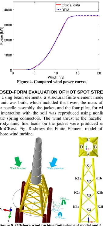
The BEM model was validated against the power curve provided by the 3.6 MW wind turbine manufacturer [12] for the full range of normal operating conditions, taking into consideration cut-in, cut-out, and supra-nominal (pitch control) wind velocities, and was found to correlate very well with the official data (Fig. 4).
Figure 4. Compared wind power curves
CLOSED-FORM EVALUATION OF HOT SPOT STRESS Using beam elements, a structural finite element model of the unit was built, which included the tower, the mass of the rotor nacelle assembly, the jacket, and the four piles, for which the interaction with the soil was reproduced using nonlinear elastic spring connectors. The wind thrust at the nacelle and hydrodynamic line loads on the jacket were produced using HydroCRest. Fig. 8 shows the Finite Element model of the offshore wind turbine.
Figure 8. Offshore wind turbine finite element model and CF expressions for load parameters at the mudline.
The computation time required to conduct the static Finite Element Analyses was approximately 0.5 s per time step, which would require several weeks of computations for the millions of wind and wave induced load cycles to simulate during a 20- year design life. To facilitate more rapid fatigue life
assessments, a faster approach was adopted which derived the Closed-Form (CF) expressions of the nominal stresses at the jacket structure‟s tubular joint connections as a function of four global load parameters (Fig. 8, left), namely:
–the amplitude and direction of the hydrodynamic load (wave/
current on jacket) induced overturning moment at the mudline (OTMHydro and βHydro), and
–the amplitude and direction of the wind load induced over- turning moment at the mudline (OTMWind and βWind).
These CF expressions were derived from structural stress assessments at the joints conducted through static FEAs for more than 8000 wind/hydrodynamic load combinations, for which a unique regression expression was fitted at the joints‟
connections through a set of constant parameters (C1 to C8), as given by Eq. (10).
2 7 8
6
5 4
3 2
1
C OTM C OTM C
C cos C C cos C OTM C
Hydro Hydro
Hydro Wind
Wind nom
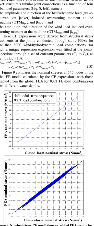
(10) Figure 9 compares the nominal stresses at 545 nodes in the global FE model calculated by the CF expressions with those extracted from the global FEA for 8321 FE-load combinations at two different water depths.
Figure 9. Nominal stress CF predictions vs. global FEA results for average high-tide (top) and low-tide (bottom) water depth FE-load
cases.
The CF expressions were derived using the FE-results corresponding to the average high-tide water depth FE-load cases, and Fig. 9 (top) shows that the CF predictions for this water depth were very accurate. The same CF expressions were then employed to calculate the nominal stresses computed for the low-tide FE-load cases, and in Fig. 9 (bottom), it appeared that the accuracy was still satisfactory despite a hydrodynamic line load distribution obtained for a 3.5 m shallower water depth. The CF nominal stress expressions approach enabled a significant reduction of the computation time to just 0.722 ms per time step. Finally, the hot spot stresses at 16 spots around the circumference of the considered connection were obtained by including the stress concentration factors (SCFs) described in DNVGL [14].
FATIGUE ASSESSMENT
This study examined the fatigue life of 6 K-joints on each face of the jacket (Fig. 8, right). These joint locations were deemed sufficiently remote from the tower flange and pile sleeve connections, approximated in the FE model by rigid kinematic couplings, that the nominal stress approach would provide sufficient accuracy for the fatigue analysis at these joints. The hot spot stresses were then calculated at 16 spots around the circumference of the intersection of the brace and chord according to DNVGL [14] formulations.
First, the time-domain load generation settings were calibrated so as to optimize the computation time while maintaining high accuracy for the fatigue assessment. To that end, our calibration study assumed a wind speed of 17.5 m/s as
„most contributing‟ due to its relatively high probability of occurrence combined with the large fluctuations (standard deviation) of its resulting aerodynamic loads.
The probabilities and standard deviations of the resulting loads of all considered wind speeds are summarized in Table 1, below (as well as in Fig. 14, which shows the relationship between these parameters and our final results). Below the wind turbine's rated wind speed of 12 m/s, the standard deviation of the wind loadload is proportional to the square of
U, which increases linearly with Uhub. In the supra-nominal wind speed range, pitch control is activated and the rate of increase of load is far more gradual up to the wind turbine‟s cut-out wind speed, whereafter the rotor is parked (feathered), and load plummets to 2% of its maximum value.
Table 1. Wind speed probabilities and standard deviations Speed
[m/s] Mode Probability
[%]
Standard deviation [kNm]
2.5 Cut-in 20.0 100.1 7.5
Normal operation
32.3 2916.5
12.5 21.3 11060.7
17.5 12.1 13366.4
22.5 9.1 15882.1
27.5 Cut-out 5.3 332.9
For this most contributing wind speed of Ucrit = 17.5 m/s, a sensitivity study was conducted to evaluate the accuracy of the fatigue damage prediction in terms of the following short-term environmental condition settings:
–short-term duration (t): 10, 20, 30, 40, 50, and 60 minutes;
–time-step interval (Δt ): 0.25, 0.5, 1.0, and 1.5 seconds.
The reference computation comprised a 60-minute load duration, which is consistent with the observations in the scatter diagrams, and a 0.25 s time-step, which enabled the wind/wave load models to capture very short load fluctuations such as tower effects and the smallest component wave loads.
The stress range distribution was then obtained by the Rainflow stress cycle counting method, and the fatigue damage was calculated from the „T‟ class S-N curve provided by DNVGL [14]. Finally, since the short-term environmental condition durations were in the order of minutes, it was necessary to artificially scale up the short-term damage DST to the 20-year design life via Eq. (11):
D20yrs =20× 365.25× 24× 60
t DST (11)
Table 2 lists the damage results, with the accuracy of the results given in terms of the reference damage Dref, computed for duration tref = 60 min and time-step Δtref = 0.25 s.
Table 2. Fatigue damage accuracy
t [min] Δt [s] Ntime-step DST D20yrs %accuracy 10 0.25 2400 2.220×10⁻⁷ 0.234 91%
10 0.5 1200 2.218×10⁻⁷ 0.233 91%
10 1 600 2.067×10⁻⁷ 0.217 85%
10 1.5 400 1.910×10⁻⁷ 0.201 79%
20 0.25 4800 4.552×10⁻⁷ 0.239 94%
20 0.5 2400 4.475×10⁻⁷ 0.235 92%
20 1 1200 4.356×10⁻⁷ 0.229 90%
20 1.5 800 3.874×10⁻⁷ 0.204 80%
30 0.25 7200 8.210×10⁻⁷ 0.288 113%
30 0.5 3600 8.095×10⁻⁷ 0.284 111%
30 1 1800 7.508×10⁻⁷ 0.263 103%
30 1.5 1200 7.308×10⁻⁷ 0.256 100%
40 0.25 9600 9.652×10⁻⁷ 0.254 99%
40 0.5 4800 9.534×10⁻⁷ 0.251 98%
40 1 2400 9.036×10⁻⁷ 0.238 93%
40 1.5 1600 8.238×10⁻⁷ 0.217 85%
50 0.25 12000 1.154×10⁻⁶ 0.243 95%
50 0.5 6000 1.126×10⁻⁶ 0.237 93%
50 1 3000 1.084×10⁻⁶ 0.228 89%
50 1.5 2000 1.106×10⁻⁶ 0.233 91%
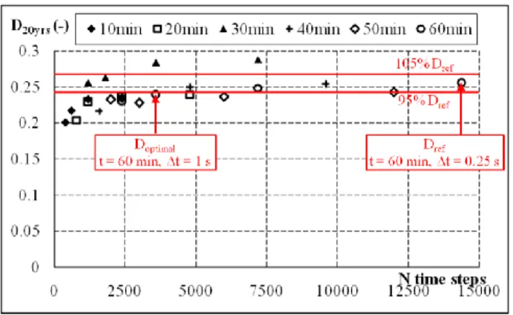
60 0.25 14400 1.457×10⁻⁶ 0.255 100%
60 0.5 7200 1.419×10⁻⁶ 0.249 97%
60 1 3600 1.364×10⁻⁶ 0.239 94%
60 1.5 2400 1.315×10⁻⁶ 0.231 90%
Fig. 10 shows the fatigue damage predictions and their related numbers of time steps, N = t × 60 / Δt, which represent the computation times. It can be observed that, except for the results obtained for t = 30 min, all the fatigue damage results tend to converge towards the reference damage Dref.
Figure 10. Damage prediction vs. time of computation for various load settings.
Figure 11 shows the stress range distributions for all short- term durations with Δt = 0.25 s. For the short-term durations of 10 min, 20 min and 30 min, the distributions deviate from that assessed by the reference computation (tref = 60 min), whereas for 40 min and 50 min, the distributions are almost identical.
This is consistent with the observations made in Fig. 10, where the damage prediction accuracy is higher for the 40 min and 50 min short-term durations. However, for probabilities of exceedance less than 10-3 (Fig. 11), the number of cycles is very low, entailing higher statistical uncertainties, which explains the large discrepancies between results in this area. Be that as it may, the fatigue prediction should not be significantly influenced by these seldom occurring conditions.
Figure 11. Stress range distribution for various short-term durations and a time-step interval of 0.25 s.
In Fig. 10, it appeared also that for larger time-steps, the damage prediction deviations from the reference value Dref remained satisfactory, while the number of time steps, and thus the computation time, dropped significantly. This is confirmed by Figure 12, which shows the stress range distributions for various time-step intervals with t = 60 min. It may be observed that the shape of the distributions remained unchanged, but the curves are translated to higher probabilities of exceedance, thereby eliminating the small stress cycles from the Rainflow counting scheme. In view of the fatigue damage prediction in Fig. 10, the contribution of the small stress cycles to fatigue may therefore be neglected.
Figure 12. Stress range distribution for various time step intervals and a simulated duration of 60 min.
From all the settings investigated, a short-term duration of t = 60 min and a time-step of Δt = 1 s were found to produce a good tradeoff between accuracy (95%) and computation speed (3600 time-steps). This optimal setting was adopted to generate the wind/wave loads for the fatigue assessment of the jacket.
For each of the 8640 short-term conditions (see Section 1), the fatigue damage was then evaluated as previously described, with the total fatigue damage calculated as the sum of all these damages weighted by their corresponding long-term statistical frequencies. Figure 13 and Table 3 present the fatigue damage results for the jacket's tubular K-joints. It can be observed that the most critical joints were 'K3a' and 'K3b' which were located low in the jacket and thus underwent higher levels of stresses, especially from the legs. However, the largest evaluated damage of 0.084 is much lower than the limit criterion of 1/3 defined by DNVGL [5] for submerged details. Therefore, the fatigue life of the investigated critical joints is sufficient.
Figure 13. Stress range distribution for various time step intervals and a simulated duration of 60 min.
Table 3. Fatigue damage results Tubular
joints
Fatigue damage for 20 years design life (-) Face A Face B Face C Face D
K1a 0.007 0.038 0.007 0.038
K1b 0.058 0.012 0.058 0.012
K2a 0.002 0.026 0.002 0.026
K2b 0.025 0.002 0.025 0.002
K3a 0.012 0.049 0.012 0.049
K3b 0.084 0.004 0.083 0.004
A further conclusion which may be drawn regards the orientation of the jacket structure. For this study, Face A of the jacket was arbitrarily oriented North-South. In the Taiwan Strait, however, the dominant wind and wave direction is North-North-East. The leg adjacent to Faces A and B and that adjacent to Faces C and D would thus be more exposed to the dominant loads. This is confirmed by the locations of the critical fatigue damages summarized in Table 3. Therefore, to increase the fatigue capacity of the jacket, Face A should be oriented North-North-East to South-South-West.
Finally, Fig. 14 shows the wind speed contribution to the fatigue damage of the K-Joints in Face A of the jacket. It can be seen that the most contributing wind speed is U = 22.5 m/s, despite having a probability of occurrence of just 28.2% of the most frequently occurring wind speed U = 7.5 m/s. However, the standard deviation of the wind load (indicative of the wind load fluctuations) at 22.5 m/s is 445% higher than that at 7.5 m/s. Ultimately, the fatigue damage produced by the wind speed U = 7.5 m/s is negligible when compared with that produced by more severely fluctuating wind speeds, despite the former having a considerably higher number of stress cycles (as indicated by its probability). It may therefore be concluded that, in addition to the numbers of stress cycles, the fatigue life is also highly sensitive to the degree of fluctuation of the wind loads, which is a function of the standard deviation of the wind speed, U, as well as the aerodynamic characteristics of the target rotor.
Figure 14. Wind speed contribution to the fatigue damage of K- Joints in the Face A of the jacket.
CONCLUSIONS
This study presented a fatigue life evaluation methodology for fixed-type offshore wind turbine foundations using time- domain simulations and the Rainflow Cycle Counting method.
A long-term statistical environment, based on a preliminary site survey comprising three years‟ worth of one-hour observations served as the basis for a convergence study for an accurate fatigue life evaluation. Short-term conditions based on IEC and DNV guidelines were generated for a number of load durations and time steps as a sensitivity study on the fatigue damage prediction. From this sensitivity study, an optimal load setting of 60-minute short-term environmental conditions with one-
second time steps was then selected. After analysis, a sufficient fatigue strength was identified, but further calculations involving more extensive long-term data measurements are required in order to confirm these results. Finally, this study highlighted the sensitivity of the fatigue life to the degree of fluctuation (standard deviation) of the wind loads, as opposed to the mean wind loads, as well as the importance of appropriately orienting the jacket foundations according to prevailing wind and wave conditions.
REFERENCES
[1] “Offshore Wind Farms Database,”
http://www.4coffshore.com, 2015
[2] T.Y. Lin, Y. Quéméner, “Extreme Typhoon Loads Effect on the Structural Response of Offshore Meteorological Mast and Wind Turbine”, Proceedings of the ASME 2016 35th International Conference on Ocean, Offshore and Arctic Engineering, OMAE2016, 19-24 Jun., 2016, Busan, Korea.
[3] B. Nelson, T.Y. Lin, Y. Quéméner, H.H. Huang, C.Y. Chien,
“Extreme Typhoon Loads Effect on the Structural Response of an Offshore Wind Turbine”, Proceedings of 7th PAAMES and AMEC2016, 13-14 Oct., 2016, Hong Kong.
[4] T.Y. Lin, Y. Quéméner, B. Nelson, H.H.Huang, C.Y. Chien,
“Fatigue Life Evaluation using Time-domain Simulation for Bottom-fixed Jacket Foundation of Offshore Wind Turbine”, Proceedings of 2016 Taiwan Wind Energy Conference, 1 Dec., 2016, Keelung, Taiwan
[5] DNVGL (2014), Design of Offshore Wind Turbine Structures, DNVGL-OS-J101.
[6] IEC, Wind turbines − Part 1: Design requirements, IEC International Standard 61400-1, 2005.
[7] Hasselmann, K., Barnett, T.P. et al., “Measurements of wind-wave growth and swell decay during the Joint North Sea Wave Project (JONSWAP)” TU Deft, 1973.
[8] Jocelyn Frechot “REALISTIC SIMULATION OF OCEAN SURFACE USING WAVE SPECTRA”
[9] “Nvidia CUDA C Programming Guide”, NVIDIA, 2014 [10] Ministry of Economic Affair of Taiwan (R.O.C.), "風力發
電 離 岸 系 統 示 範 獎 勵 辦 法 (Regulations for Demonstration and Rewards of Offshore Wind Power System)", Taiwan, 2012.
[11] L. Kristensen, G. Jensen, A. Hansen, and P. Kirkegaard,
“Field Calibration of Cup Anemometers”, Risø–R–
1218(EN), Risø National Laboratory, Roskilde, Denmark, 2001
[12] Siemens brochure, “Thoroughly tested, utterly reliable:
Siemens Wind Turbine SWT-3.6-120”, Germany, 2011.
[13] M. Hansen, Aerodynamics of Wind Turbines, 2nd Ed., Earthscan, London, UK, 2007.
[14] DNVGL (2016), Fatigue design of offshore steel structures, DNVGL-RP-C203
[15] L. Johansson, The importance of data availability: Effects of missing or erroneous data, EWEA 2013, Vienna, Austria