無線感測網路中跳躍數導向位置估算演算法之研究

(1)

行政院國家科學委員會專題研究計畫成果報告

無線感測網路中跳躍數導向位置估算演算法之研究研究成果報告(精簡版)

計畫類別：個別型

計畫編號： NSC 96-2221-E-011-038-

執行期間： 96 年 08 月 01 日至 97 年 09 月 30 日執行單位：國立臺灣科技大學電子工程系

計畫主持人：陳省隆

計畫參與人員：碩士班研究生-兼任助理人員：鍾惠如碩士班研究生-兼任助理人員：路艾妮碩士班研究生-兼任助理人員：彭崇聖碩士班研究生-兼任助理人員：鄭福輝

報告附件：出席國際會議研究心得報告及發表論文

處理方式：本計畫涉及專利或其他智慧財產權，1 年後可公開查詢

中華民國 97 年 12 月 23 日

(2)

行政院國家科學委員會專題研究計畫成果報告

無線感測網路中跳躍數導向位置估算演算法之研究

A Hop-Oriented Position Estimation Algorithm for Wireless Sensor Networks

計畫編號：NSC96-2221-E-011-038- 執行期限：96 年 8 月 1 日至 97 年 9 月 30 日

主持人：陳省隆教授國立台灣科技大學電子工程系共同主持人：

計畫參與人員：鍾惠如、路艾妮、彭崇聖、鄭福輝

一、中文摘要

無線感測網路 (Wireless Sensor Networks，WSN)是由一群感測節點(sensor nodes)所組成的網路結構，感測節點將感測環境所得之資料藉由無線電波 (Radio Frequency，RF)廣播到基地台(base station)。

由於感測節點所感測的資料必須和位置結合，才有實用的價值，因此在無線感測網路裡估算位置變成一個重要的議題。理想上，

讓每個感測節點都裝配全球衛星定位系統 (Global Positioning System，GPS)便可以得到位置，然而此方法太花費成本，並與原本感測節點的低成本(low cost)目標不合。因此較合理的解決方法是讓少數感測節點擁有 GPS，其餘的感測節點利用蒐集到的位置資訊，去估算出本身的位置。

本研究計劃旨在提出跳躍數導向位置估算(Hop-Oriented Position Estimation，HOPE) 演算法，四個裝配GPS 的信標節點廣播跳躍數資訊，一般節點利用跳躍數資訊，搭配能在感測節點計算的簡易運算式，來獲得較準確的估算位置。

關鍵字：感測節點、全球衛星定位系統、低成本、廣播、跳躍數、信標節點、一般節點。

Abstact

A wireless sensor network consists of a group of sensor nodes that broadcast the sensed

data to the base station hop by hop via radio frequency. It is useful only if the sensed data are associated with the locations of the sensor nodes. Therefore, location estimation of sensor nodes becomes an important issue. Ideally, each sensor node can obtain its location by being equipped with a GPS device each.

However, it costs too much, contradicting the object of low cost of sensor nodes. Hence, it is reasonable that few sensor nodes are equipped with a GPS device each and the others estimate their locations by collected information.

The purpose of this thesis is to propose a hop-oriented position estimation algorithm (HOPE). Four beacon nodes equipped with GPS broadcast the hop count information.

Normal nodes employ the hop count information to estimate their position more closely with simple calculations.

Keywords: sensor node, GPS, low cost, broadcast, hop count, beacon nodes, normal nodes.

二、緣由與目的

由於近來微型製造技術、通訊技術及嵌入式處理技術的迅速提升，使得微小的電子裝置可以內嵌精密感測(sensing) 、通訊 (communication)與計算(computation)等多樣化功能，這樣的裝置稱為感測節點(sensor node)[1]，此類感測節點不但能偵測及感應環境的變化，更能將所蒐集到的資訊分析，且

(3)

透過無線通訊的功能將資料傳送至資料收集中心或是基地台(base station)；由於感測節點的硬體設計以低成本(low cost)、體積小與低耗電為主要考量，因此節點本身所配備之電源、記憶體以及運算能力均受到極大的限制。感測節點主要由四個部分組成，分別為感測單元、計算單元、通訊單元以及供電單元，如圖1。

圖 1 感測節點示意圖

無線感測網路(wireless sensor network，

WSN) 是一種由大量感測節點所構成的網路，在應用方面十分廣泛，許多如軍事(監控戰場上的狀態)、環境感測(如森林火災、化學物偵測)、醫學(如心跳、血壓量測)以及災害偵測(如龍捲風、地震)等，都可以看到無線感測網路的應用。在 WSN 上，不同的應用會有不同的設計，一個想要觀測某地區現象的 WSN 系統架構如圖 2 所示，首先將大量的感測節點散佈在待感測區域來蒐集各種環境資料，再利用無線網路將蒐集的資訊交給基地台，管理者或使用者透過網際網路可以從基地台獲取資訊。

圖 2 無線感測網路示意圖

當 WSN 興起之後，此種技術逐漸被廣泛使用，然而 WSN 為一種特殊之隨建即用的無線網路，感測節點擔任感測環境、資料分析與繞送的工作，由於節點是隨機的分佈於待測區域中，所以節點感測到的資訊，都必須和節點所處的位置(position)結合才有意義，因此想要正確且有效率的利用這些資

訊，應該如何更精確且合理的取得感測節點的位置，是一個值得去研究的重要議題。

在 WSN 中想要獲得位置資訊，某些研究直接假設感測節點本身就擁有此位置資訊，但是只能夠在小範圍或是感測節點分佈規律下，才有可能實現；近年來，由於全球衛星定位系統(Global Positioning System，

GPS)[2]的發展，因此可以假設讓所有的感測節點都擁有 GPS，藉此獲得位置資訊，但是 GPS 的價格比較昂貴，並不符合感測節點的低成本考量；所以近年來的研究之中，將部分感測節點搭配 GPS 來獲得本身的位置資訊，其他的感測節點藉由蒐集鄰近的位置資訊來估算出位置，是一個比較合理的解決辦法。

考量感測節點的記憶體以及運算能力，

實際上感測節點的功能無法太強大，然而要如何利用所蒐集到的資訊，去取得本身的位置資訊，常見的有二種方式，首先是集中式 (centralized)演算法，將資訊全部交給基地台估算，並且由基地台廣播取得位置資訊，集中式演算法雖然能獲得較準確的位置，但是由於要將資訊交由基地台處理，所以在訊息的交換上負擔很重；因此，另一種分散式 (distributed)演算法被提出，盡量的將計算式簡化，使得在感測節點上，能夠直接將蒐集到的資訊估算出位置，在準確性不會太差的情況下，有效的解決訊息交換的負擔。

根據之前被提出方法中，我們將裝備 GPS 擁有位置資訊的感測節點稱為信標節點 (beacon node)，而其他沒有位置資訊需要被估算的感測節點，稱為一般節點(normal node)；在本篇論文中，提出了跳躍數導向位置估算(Hop-Oriented Position Estimation ， HOPE)演算法，使用數個信標節點發送跳躍數，一般節點則利用蒐集到的資訊，估算出本身的位置。

三、研究方法

在最近幾年已有許多的位置估算演算法被提出，這些演算法主要可以分為以下二種類型：

(4)

1. Range-based 定位法

Range-based 定位法，主要是藉由求得距離和角度的資訊，來估算出位置的方法；例如使用信號到達時間(Time of Arrival ， TOA)，感測節點發出信號，接收者接收此信號並利用傳遞的時間[3]，大致估算出兩者之間的距離，但是由於感測節點間時間同步化的問題，將會重大的影響準確度。此外使用信號到達時間差(Time Difference of Arrival，

TDOA)[4][5][6]，大致的方法和 TOA 相同，

但是感測節點上擁有兩種不同的電波頻率，

利用超音波(ultrasound)以及無線電波(RF)的傳送，可用來解決時間同步的問題，接收信號的節點獲得不同電波頻率到達的時間，計算出二者的差距，估算出相對的距離。TOA 以及TDOA 都是利用信號傳送的時間來決定距離，但是在無線感測網路之中，信號的傳送時間，有可能因為網路的環境而受影響，

因此這類演算法並不是理想的方式。

另外信號到達角度(Angle of Arrival，

AOA)，主要是用來得到相對的角度之用，利用方向性天線(directional antenna)或是數位羅盤(digital compass)[7]來實作，可以得到感測節點間相對的角度，通常此方法會搭配 TOA 或是 TDOA 使用，來達到更精確的估算，但是此方式需要某些較昂貴的硬體配備，因此也不適合在無線感測網路中使用。

最後，利用參考接收信號強度(Received Signal Strength Indicator ， RSSI)[4][8][9][10][11][12]，這種方式主要是利用傳送的信號強度，以及接收到信號的強度，考慮信號衰減的情形，利用方法去估算出傳送端和接收端的距離。計算方式為

0

( ) 10 log_p d

P d P n

= − d ，此為傳送了一小段參考距離所接收到的信號強度(dBm)。在信號傳遞的過程中，有許多的外在因素，會影響信號的強弱，因此接收到的信號強度，

並無法完全的代表相對的距離，因此這種演算法並不理想。

P0

d0

2.Range-free 定位法

由於range-based 定位法，通常需要較昂

貴的設備來換取更準確的定位，因此在講求低功率低成本的無線感測網路中，提出了一種不需昂貴設備去換取精確的距離或角度，

花費較小的range-free 定位法。

近年來使用 range-free 的方法不斷被提出，例如DV-Hop[7][13]，將擁有位置資訊的感測節點，稱為Anchor，Anchor 廣播出包含自己位置資訊的封包，採取類似距離向量路由(DV-routing)的方式，感測節點記錄著最小的跳躍數(hop count)，多個 Anchors 都依此方法實行後，感測節點皆會取得到 Anchors 最小跳躍數表格(hop count table)，之後 Anchor 會計算本身到其他 Anchors 的距離，與其他 Anchors 的跳躍，計算出單一跳躍距離，並將此資訊廣播，當節點蒐集此資訊，可將此資訊配合之前記錄的跳躍數表格，即可計算出到所有 Anchors 之相對距離，當有三個 Anchors 的相對距離以及座標，便可使用三角測量法估算出自己的位置。然而，此種方式必須在整個環境較密集的(dense)情況下才能發揮效用，並且需要大量的訊息交換，增加系統負擔。

GRIPHON 演算法[14]也利用了跳躍數來幫助估算位置，將四個參考用的節點固定放置於感測區域的四個角落，稱之為 marker，marker 發送訊息讓在區域內的感測節點收集最小跳躍數，並將四個跳躍數集合成跳躍數向量(hcv)，之後交由控制中心與分成小格子(grid) 的感測區域比對跳躍數向量，由於控制中心已知所有格子的跳躍數向量，因此可將感測節點定位在最符合的格子中心點；此方式利用跳躍數向量與所處位置的關係來定位，因此跳躍數向量的誤差必須不能太大，所以需要感測節點很密集的環境下，才能夠得到較好的結果。

圖 3 GRIPHON 示意圖

Convex Position Estimation(CPE)演算法 [15]，假設一般節點聽到附近信標節點的廣播，則可以認定本身是位於此信標節點的傳

(5)

輸範圍之中，當同時聽到多個信標節點的廣播，則可以認定位於數個信標節點傳輸範圍交集之中，如圖4 所示；CPE 主要是由基地台處理節點多種的資訊，計算出最佳化的凸狀交集，並提出了估算的矩形(Estimative Rectangle)，將可能的交集範圍用矩形涵蓋，

計算出矩形的中心點成為估算位置。然而，

由於要最佳化凸狀交集的計算複雜，因此必須經由基地台計算，再將位置資訊發送給一般節點，造成訊息交換的嚴重負擔。

圖 4 CPE 交集示意圖

圖 5 估算的矩形示意圖

分散式位置估算 (Distributed Location Estimation，DLE)演算法[16]，此方法與 CPE 概念相同，利用了估算的矩形，並且使用簡易的計算，將計算交由各個節點，減少基地台與節點間訊息交換的負擔；DLE 並提出了遠端鄰居信標節點(farther neighboring beacon node)來更精確的估算位置，信標節點可以用較大的電波傳輸範圍來互相溝通蒐集資訊，

並把此資訊告訴需要估算位置的節點，則此節點可以將遠端鄰居信標節點所涵蓋的交集範圍刪去，進一步的提升精確度，如圖 6 所示。

圖 6 遠端信標節點示意圖 .跳躍數導向位置估算演算法

本的假設：

，稱為一般

節點都擁有獨一無二的身分佈。

1β、2β、

β、6β 的廣播區域皆座標化。

估算出準確的

3.1 收集資訊

算法中主要使用的估算資訊，

即為

3

HOPE 演算法有以下幾個基

(1) 裝配 GPS 的感測節點能夠取得本身位置，稱為信標節點。

(2) 未裝配 GPS 之感測節點

節點。

(3) 每個感測分(unique ID)。

(4) 感測節點是隨機的

(5) 信標節點擁有傳輸半徑為

3β、4β、5β、6β 的廣播能力，其中 β 為傳輸的單位距離。

(6) 一般節點則擁有 4β、5 能力。

(7) 假設整個

為了能使用較少的信標節點，

位置，提出了跳躍數導向位置估算演算法。HOPE 演算法分成二個步驟，首先是收集資訊，四個信標節點分別廣播出位置以及跳躍數；之後則是估算位置，一般節點則依照所接收的跳躍數資訊，估算出本身位置。

HOPE 演

節點至各個信標節點的跳躍數，為了讓擔任發送跳躍數的信標節點，能夠分散在區域的四個角落，使跳躍數能夠來自不同的方向，因此假設可以將整個區域區分成九宮格，信標節點則限制在每個角落中隨機分佈。如圖7 所示。

圖 7 HOPE 使用的 WSN 示意圖

在化是

件困

3.1.1

(所有節點取 WSN 中，將感測節點時間同步難的事，因此在 HOPE 演算法中，由基地台來控制感測節點；當選基地台發出通知訊息，告知其中一個信標節點，可以開始發送跳躍數資訊了，在傳送通知訊息的過程中，收到此訊息的節點，若不是被通知的信標節點，則只將訊息轉送出去，當此信標節點接收訊息後，便開始依序廣播跳躍數。

信標節點廣播

當基地台等待了一段時間

得到此信標節點的跳躍數) 後，便會通知下

(6)

一個信標節點發送跳躍數，依此類推，直到所有節點皆收到至四個信標節點的跳躍數。

以其中一個信標節點的情況來說明，信標節點首先使用傳輸半徑為 1β 的電波廣播含有跳躍數為 1 的訊息，接收到的節點即記錄跳躍數為 1，依此類推，再度改變傳輸半徑為 2β、3β、4β、5β 和 6β，收到這些廣播的節點則記錄這些訊息，其跳躍數分別為2、3、4、

5 和 6；每個感測節點會記錄此信標節點的座標及最小跳躍數，由於是信標節點直接廣播的訊息，所以在6β 傳輸範圍中的節點，如同圖 8 所示，跳躍數將依照傳輸半徑的不同，

與圓環相對應。

圖 8 信標節點廣播示意圖 .1.2 其他節點廣播

3

由於希望其他轉播跳躍數的節點，能由內向外一層層的傳送，減少廣播碰撞的問題，因此設定了播放時段機制，理想上節點將依照記錄的跳躍數，在可撥放的時段內廣播跳躍數資訊；信標節點在時段 0 中，廣播 1 至 6 跳躍數資訊；若節點的跳躍數記錄為 1 時，會在時段1 內連續廣播 1+4、1+5 及 1+6 三種跳躍數訊息，依此類推，若節點跳躍數為k，則會在時段 k 內廣播 k+4、k+5 及 k+6 三種跳躍數訊息，廣播時段 m，可依照感測區域的大小計算出m，如圖 9。

圖 9 播放時段示意圖

傳送的訊息，除了跳躍數資訊和信標節點座

時間標之外還包含發送者的跳躍數，以及剩餘時間(發送者將該時段結束時間與本身隨機廣播時間計算)；當有節點收到此訊息，想要知道自己時段的開始時間，則會利用相差的跳躍數計算需等幾個時段，並加上剩餘時間，則可計算出等待時間，當等待時間結束時，此時即為本身跳躍數可開始廣播的時段，節點會在此時段中隨機選擇廣播時間廣播，若是在等待時間結束前收到更小的跳躍數訊息，則會重新計算等待的時間。

利用相對時間控制，會有類似節點同步化的功效，節點將會依照本身的跳躍數，在適合的時段內廣播，在理論上，播放時段可以讓廣播如同水波般，由中心點一層層依序的向外擴散，減少不同層的碰撞發生；在可廣播時段中隨機選擇時間後播放，

也可以減少同層間的碰撞，碰撞的機率降低，所獲得的跳躍數就更理想了。

圖 10 計算等待時間示意圖 .1.3 跳躍數向量與向量區塊

、D)都完成廣播後

情形，參考 3

當四個信標節點(A、B、C

，每個感測節點理論上，皆會獲得到達四個信標節點的最小跳躍數，(h(A)、h(B)、

h(C)、h(D))即為跳躍數向量。

考慮某一信標節點廣播覆蓋

節點以六種傳輸半徑電波廣播，其覆蓋範圍為六個半徑不同的同心圓，如圖 8 所示。跳躍數為 1、2、3…的節點，依序以三種不同傳輸半徑電波廣播，第七層以後的圓環會像洋蔥似依序產生；以三種不同傳輸半徑電波廣播，主要是要讓第六層後的圓環厚度較為均勻，並且希望能夠達到接近於理想同心圓的分布，以增加演算法的準確度。當以四個信標節點的同心圓來考慮時，四個洋蔥圖重疊後，將整個區域切割成數個形狀不一的區塊，相同區塊內的節點有相同的跳躍數向量，將這些特殊的區塊稱為向量區塊。圖11 為理想情況下，所形成的向量區塊示意圖。

(7)

圖 11 理想同心圓形成向量區塊示意圖 .2 估算位置

取得跳躍數向量之後，基地台便會

信標節點的跳躍數，

節點圓環交集

.2.1 類似平行四邊形(quasi-parallelogram) 生幾

行四邊形的各組

圖12 所示，假設節點位於待估算向量區塊

3

當節點皆

發出位置估算通知，節點則可利用跳躍數向量以及信標節點的座標，配合向量區塊的概念，將位置估算出。

向量區塊是依照至四個

所對應圓環交集出的區域，每塊向量區塊皆由四個圓環交集所形成，並擁有一組獨一無二的跳躍數向量；因此，藉由將整個區域細分成多個向量區塊，並以簡單的方式，

估算向量區塊的中心點當作估算位置，便是 HOPE 演算法的主要概念。

由於向量區塊是四個信標

所產生，為了用簡單的方式求出向量區塊的中心點，則可以先選擇二個圓環，取得圓環交集出的類似平行四邊形，並利用二圓環的中心線，相交獲得類似平行四邊形的中心點，之後選擇其中一個剩下的圓環，與類似平行四邊形取得交集區域，同樣利用圓環中心線，求出與類似平行四邊形中心點最接近之圓環中心點，將二者取中間點，則為此交集區域的中心點，最後將剩下的圓環加以考慮，與上述方式相同，將圓環與交集區域找交集，此交集即為待估算的向量區塊，將交集區域中心點與圓環中心點取中間點，此點將會接近於向量區塊的中心點，即為位於此向量區塊中節點的估算位置。

3

在找出類似平行四邊形的過程中，會發個影響準確度的情形，首先是使用任二圓環的交集，有可能會出現無法交集出分離

的二個類似平行四邊形，若是無法交集出分離的類似平行四邊形，便無法輕易的取得區域的中心點，因此，為了排除這種情形，則會將各種可能的圓環組合，依照與向量區塊所形成的夾角 θ，角度越接近直角，不但可以確保交集出分離的類似平行四邊形，並且交集出的類似平行四邊形將會越接近於矩形，在估算的時候，準確度也將會比形成菱形的類似平行四邊形更準確。

另外，在選擇交集出類似平

圓環時，由於產生的類似平行四邊形有二個，所以可藉由至其他信標節點的跳躍數選擇符合的類似平行四邊形；因此若是使用信標節點與向量區塊較接近的圓環，雖然可以有分離的類似平行四邊形，但是此分離的類似平行四邊形會較靠近，在利用至其他點的跳躍數判斷時，容易產生誤判的情形，為了避免發生這種問題，在選擇圓環之前，先將距離向量區塊最近的節點剔除，使用剩餘的三個節點來找出夾角 θ，選擇最適合的組合。

如

中，首先將接近的A 點剔除，並利用夾角θ 找出 B 與 C 的組合，之後利用二圓環的中間線，並使用至A 或 D 的跳躍數選擇合理的類似平行四邊形，所獲得的交點即為此類似平行四邊形的中心點，如圖13 所示。

圖 12 選擇二點信標節點示意圖

圖 13 類似平行四邊形示意圖

(8)

.2.2 交集區域 量區

3

由於類似平行四邊形，是將範圍內的向塊皆估算在中心點，大概的估算位置，

因此為了減去使用類似平行四邊形多考慮的區域，提高準確度，則可將剩下的信標節點，

先選擇本身跳躍數對應的圓環與類似平行四邊形交集區域較大者，所獲得的交集區域估測中心點，準確度會較高，如圖14 所示，取得交集區域的估測中心點。依此類推，最後的圓環也加以考慮，如圖15 所示，獲得的估算位置，將會接近於向量區塊的中心點，此點即為位於向量區塊中節點的估算位置。

圖 14 交集區域估測中心點示意圖

圖 15 取得估算位置示意圖 .2.3 圓環厚度不足與解決方法 節點

均勻，除

、模擬結果與分析

為了證明跳躍數導向位置估算演算法的準確

較，

將 HOPE 演算法使用了 Network

.1 感測節點密度的影響

法，選擇同樣是屬於分

4 3

由於節點隨機分布的特性，因此在信標廣播跳躍數資訊後，轉播的節點會因為本身在圓環中的位置，造成轉播後的圓環逐漸縮小，造成估算上的誤差，此種情形在節點密度不足的情況下最為嚴重。

因此為了將圓環厚度能夠變的

了讓轉播節點能使用較大的傳輸半徑之外，

並將依照節點分布的密度，加強轉播節點廣播時的能量，將傳輸範圍稍微加大，如此便能解決轉播節點位置造成的誤差，並稍微補足圓環的厚度，使形成的圓環能夠接近同心圓。

四

性及實用性，將會分成二部份來說明。

首先選擇了分散式位置估算演算法比並且使用了 C 語言分析，在假設 MAC 層能避免封包碰撞，且不考慮干擾，由於只在感測節點佈下時定位，因此也不考慮電量的消耗；將模擬的環境設定為長寬各為 1000m 的正方形區域中，改變節點數 50~250，比較平均誤差(mean error，將估算後的一般節點的位置與其實際位置算出誤差距離，統計全部的誤差距離平均)，證明準確性。

之後

Simulator version 2(NS2)來模擬，將碰撞以及時間同步化的問題加以考慮，並與使用C 語言分析之數據比較，藉由模擬數據以及分析數據的比較，可以證明 HOPE 演算法的實用性。

4

與 HOPE 比較的演算

散式的 DLE 演算法，由於 DLE 演算法需要多個信標節點，因此選擇在DLE 演算法中較佳的情況，讓信標節點占全部節點 40%

來比較，圖16 為改變感測節點數量對平均誤差的影響，從圖中可以發現，DLE 演算法在密度不夠情況下，會產生嚴重的錯誤，必須要在密度足夠的情況下，才能夠獲得較穩定的平均誤差，但是信標節點的使用，也會隨之增加，而 HOPE 演算法在各種密度下，獲得的平均誤差皆能夠比 DLE 演算法更準確；另外，圖17，為 DLE 演算法 0%及 HOPE 演算法的平均誤差範圍，由圖中可以看出，

HOPE 演算法在節點密度較高時，不但平均誤差較低，並且在每次模擬時都能接近平均值，由此可得知HOPE 演算法的穩定性較高。

雖然 HOPE 演算法在節點密度較小的情

(9)

況下，也能獲得較好的平均誤差，但是在節點密度不足時，以平均誤差範圍的觀點，可以發現誤差HOPE 演算法也會產生不穩定的情形，因此HOPE 演算法必須在足夠的密度下，才能有較好的準確性及穩定性。

圖 18 HOPE 使用 C 與 NS2 比較圖 4.3 增加演算法的準確度

藉由估算出向量區塊中心點的概念，可以推論出，若是能將向量區塊的劃分變得更細小，則向量區塊涵蓋的範圍也將會變小，

位於向量區塊內的節點，也就更接近向量區塊的中心點，估算的誤差也會隨之降低，因此，可藉由調整發送跳躍數的 β 值，將傳輸半徑縮小，圖19(a)為在較小節點密度中，將 β 由 20~50 的平均誤差比較圖，並且採用 95%

信賴區間(confidence interval)。由圖中可以得知，將 β 值變小之後，節點的密度就變得很重要，若是密度不足，準確度不但沒有變好，

反而會造成更嚴重的誤差。

圖 16 Node density vs. Mean error

圖 17 平均誤差範圍比較圖

.2 碰撞與時間同步化的影響

播訊息，來取 4

HOPE 演算法需要藉由廣

得估算位置資訊，由於實際網路中，常會有碰撞的情形發生，因此為了證明演算法的實用性，利用了NS2 來模擬，並與之前無碰撞所模擬的數據比較，如圖18 所示，從圖中可以發現，在考慮封包碰撞，並使用相對時間來達到同步化的情形下，使用NS2 模擬的曲線，雖然在密度不足時，產生碰撞後無法像密度較高時，可藉由其他轉播節點彌補，因此會比理想情況稍差，不過在密度足夠情形之下，皆會接近於使用C 語言模擬的數值，

由此可以證實，播放時段的機制，可以成功將大部分的碰撞避免，增加演算法的合理性。

圖 19(a) 改變 β 值(節點密度小) 圖19(b)則是在較大的節點密度下，調整 β 值的比較圖，並且採用 95%信賴區間。與圖19(a)比較可以發現，在節點密度足夠的情況下，平均誤差將隨著 β 值的變小來降低，

獲得更好的準確度。

從 19(a)與 19(b)可以得知，當密度小於 400 (node/km²)時，使用 β=50 可獲得較佳的平均誤差，密度400~700 時則可使用 β=40，

密度 700~1000 時則使用 β=30 ，密度 1000~5000 則使用 β=20，密度高於 5000 則推

(10)

薦使用β=10。實際佈下感測節點時，使用者可依照密度調整β 值，取得最佳的平均誤差。

圖 19(b) 改變 β 值(節點密度大) 五、計畫成果自評

在 WSN 中，為了讓感測節點所感測的資訊有意義，就必須與位置資訊結合；將少部分感測節點裝配GPS 獲得位置資訊，其他節點利用這些信標節點，獲得本身的估算位置，是一個較合理的解決方式，由於GPS 的價格高於感測節點，因此，為了降低成本，

並且獲得不錯的估算準確度，提出了跳躍數導向位置估算演算法。

在 HOPE 演算法中，利用跳躍數對應的圓環，將整個區域分成多個向量區塊，並將向量區塊的中心，當成位於此向量區塊中節點的位置，模擬的結果顯示，HOPE 演算法不但比DLE 演算法使用更少的信標節點，並且擁有較高的準確度，更可以藉由調整 β 值，符合使用者的需求；在NS2 模擬中，也發現播放時段成功的將碰撞降低，增加演算法的可信度。除了透過NS2 模擬之外，未來在實際 WSN 中實作 HOPE 演算法，也是值得繼續探討的議題。

六、參考文獻

[1] J. Hill, R. Szewczyk, A. Woo, S. Hollar, D.

Culler, and K. Pister, “System architecture directions for networked sensors,”

ASPLOS 2000, pp. 93-104.

[2] “Garmin international: about GPS”, http://www.garmin.com/aboutGPS/

[3] S. Capkun, M. Hamdi, and J. P.

HubauxInstitute, “GPS-free positioning in mobile ad-hoc networks,” HICSS’01, January 2001.

[4] J. Hightower and G. Borriello, “Location Systems for Ubiquitous Computing,”

IEEE Computer, vol. 34, August 2001.

[5] N. B. Priyantha, A. Chakraborty, and H.

Balakrishnan, “The Cricket Location-Support System,” ACM/IEEE MobiCom 2000, pp. 32-43, Boston, MA, August 2000.

[6] S. Ray, R. Ungrangsi, F. D. Pellegrini, A.

Trachtenberg, and D. Starobinski, “Robust Location Detection in Emergency Sensor Networks,” IEEE Computer and Communications Societies (INFOCOM 2003), vol. 2, March-April 2003.

[7] D. Niculescu and B. Nath, “DV Based Positioning in Ad Hoc Networks,” Journal of Telecommunication Systems, pp.

267-280, vol. 22, January-April 2003.

[8] N. Bulusu, J. Heidemann, and D. Estrin,

“GPS-less Low Cost Outdoor Localization For Very Small Devices,” IEEE Personal Communications Magazine, vol. 7, no. 5, October 2000.

[9] F. Mondinelli and Z. M. K. Vajna, “Self

Localizing Sensor Network Architectures,” IEEE IMTC/2002, vol. 1,

May 2002.

[10] N. Patwari, R. J. O’Dea, and Y. Wang,

“Relative Location inWireless Networks,”

IEEE VTC, pp. 1149-1153, Rhodes, Greece, May 2001.

[11] P. Bahl and V. N. Padmanabhan,

“RADAR: An In-Building RF-based User Location and Tracking System,” IEEE Computer and Communications Societies (INFOCOM 2000), vol. 2, March 2000.

[12] J. Hightower, R. Want, and G. Borriello,

“SpotON: An Indoor 3D Location Sensing Technology Based on RF Signal Strength,” UW CSE 2000-02-02, University of Washington, Seattle, WA, February 2000.

[13] D. Niculescu and B. Nath, “Ad Hoc Positioning System (APS),” IEEE Globecom 2001, vol. 1, November 2001.

[14] G. L. Joo and S. V. Rao, “A grid-based location estimation scheme using hop counts for multi-hop wireless sensor networks,” IWWAN 2004, University of Oulu, 2004.

[15] L. Doherty, K. S. J. Pister, L. E. Ghaoui,

(11)

“Convex Position Estimation in Wireless Sensor Networks,” IEEE Computer and Communications Societies (INFOCOM 2001), vol. 3, April 2001.

[16] J. P. Sheu, J. M. Li, and C. S. Hsu, “A Distributed Location Estimating Algorithm for Wireless Sensor Networks,” IEEE SUTC2006, vol. 1, June 2006.

(12)

會議名稱：The Fourth International Conference on Wireless and Mobile Communications 發表論文： Improving Scalable Video Transmission over IEEE 802.11e through a Cross-Layer Architecture

報告人：國立台灣科技大學電子系陳省隆教授一、參與會議經過

2008 年第四屆國際無線與行動通信會議 (The Fourth International Conference on Wireless and Mobile Communications) 自 2008 年 7 月 27 日至 2008 年 8 月 1 日在希臘雅典舉行。本會議由 IARIA 協會主辦，論文收錄在 IEEE Explore，本年度收到來自五大洲多篇論文，經過嚴格評審，被選定發表的論文品質相當高。本年度會議之主題在於 advanced wireless technologies, wireless networking, and wireless applications，在此主題下，安排了一個 keynote speech 及十一個平行議程：

(1) Protocols for wireless and mobility

(2) Performance Evaluation, Simulation and Modeling of wireless networks and systems (I) (3) Wireless and Mobile Technologies (I)

(4) Wireless and Mobile Technologies (II)

(5) Applications and services based on wireless infrastructures (I) (6) Applications and services based on wireless infrastructures (II) (7) Management of wireless and mobile networks (I), network deployment (8) Management of wireless and mobile networks (II)

(9) Performance Evaluation, Simulation and Modeling of wireless networks and systems (II) (10) Performance Evaluation, Simulation and Modeling of wireless networks and systems (III) (11) Security in wireless and mobile environment

本人於7 月30 日宣讀一篇論文，和與會專家學者意見交流，更獲得與會專家學者重視。

二、與會心得與建議

參與國際會議，不僅可以與各國專家學者作意見交流，也能激發新的研究方向，更能將論文修改後投至著名期刊，提升國內研究能量。希望國科會能提供充足經費以鼓勵參與國際會議，提升國內學術研究水準，使國內大學早日擠進世界一流大學之列。

三、攜回資料名稱及內容攜回會議論文光碟一片。

(13)

Improving Scalable Video Transmission over IEEE 802.11e through a Cross-layer Architecture

Hsing-Lung Chen, Po-Ching Lee Department of Electronic Engineering National Taiwan Univ. of Sci. and Tech., Taiwan

[email protected], [email protected]

Shu-Hua Hu

Department of Comp. Sci. and Info. Eng.

Jiwen Univ. of Sci. and Tech. Taiwan [email protected]

Abstract

The scalable extension of H.264/AVC, called H.264/SVC, is a current standardization project of Joint Video Team (JVT). An encoded SVC bitstream consists of an H.264/AVC-compatible base layer and one or more scalable enhance layers. In order to meet requirements of various clients, some scalable enhance layers can be truncated. This paper focuses on the investigation of H.264/SVC transmission over IEEE 802.11e through a cross-layer architecture. The cross-layer architecture, enabling interaction between Network Abstraction Layer (NAL) and IEEE 802.11e MAC layer, provides differentiated services according to the importance of scalable video packets. The simulations are conducted with Qualnet 4.0. The simulation results show that our approach provides better video quality.

1. Introduction

In recent years, with the development of two high-speed physical (PHY) layers, IEEE 802.11g (54 Mb/s) [1] and IEEE 802.11n (100 Mb/s) [2], there is a growing need for multimedia services over WLANs (e.g. download-and-play, video conferencing, video streaming, video broadcasting, etc). However, 802.11 WLANs can only provide best-effort service, which would restrict the Quality-of-Service (QoS) for multimedia services. Therefore, a new standard, so- called IEEE 802.11e [3], defines the MAC procedure to support different kinds of traffics (voice, video, best-effort and background) over WLANs. The IEEE 802.11e standard introduces the Hybrid Coordination Function (HCF) and specifies two access schemes: the Enhanced Distributed Channel Access (EDCA) and the HCF Controlled Channel Access (HCCA).

In the same time, Joint Video Team (JVT) of International telecommunication Union Telecom (ITU-T) and Moving Picture Experts Group (MPEG) continues improving the coding efficiency over existing standards (as shown in Figure 1). H.264/AVC [4], which is the most recent coding standard, attracts attention from many researchers because it can provide gains in coding efficiency

of up to 50% over a wide range of bit rates and video resolutions compared to previous standards [5]. H.264/AVC conceptually consists of the video coding layer (VCL) and the network abstraction layer (NAL). By recording the network status in NAL units, VCL has the capability of error-resilience.

Figure 1. Chronological progression of ITU and MPEG standards [6]

In fact, it is not easy to deliver video streams over wireless networks, because the data rate of video is much bigger than that of voice and there are some problems in wireless environment, such as fading, the stability of bandwidth, bit error and packet loss. In heterogeneous networks, different users have different requirements, such as bandwidth and video quality and resolution. Therefore the streaming server usually needs to prepare multiple encoded versions of each video for diverse clients and delivery networks. It needs huge storage capacity to maintain multiple versions of video streams. To avoid the drawbacks of the conventional approaches, JVT is currently standardizing Scalable Video Coding (SVC) standard, which can provide the function of universal multimedia access (UMA) [7], as the latest amendment of H.264/AVC.

At the time of writing, the most recent draft of SVC is available in [8] and the final draft is scheduled in April 2007.

This paper focuses on the efficient transmission of H.264/SVC video over IEEE 802.11e WLANs by proposing a cross-layer architecture on both application layer and MAC layer. The proposed cross-layer architecture relies on the different importance of NAL units and a differentiated mapping at the MAC layer. Based on the QoS requirement of those different NAL units, we specify a mapping algorithm at the MAC layer that associates each NAL unit The Fourth International Conference on Wireless and Mobile Communications

241

The Fourth International Conference on Wireless and Mobile Communications

241

(14)

with an access category (AC). Thus, we allow the allocation layer to pass its SVC streams along with their requirements in order to protect the most important H.264/SVC information, resulting in low degradation for received H.264/SVC streams.

This paper is organized as follows. In section 2, we introduce the basic concept of SVC. Section 3 introduces IEEE 802.11e and cross-layer video transmission. Section 4 describes the proposed cross-layer architecture and mapping algorithm. Section 5 presents the simulation results. Finally, we conclude our work in section 6.

2. Scalable video coding (SVC)

The basic SVC design, which is an extension of the H.264/AVC video coding standard, can be classified as layered video codec. Figure 2 shows a coding structure with two spatial layers each of which contains a fine grain SNR scalability enhancement layer. After this coding process, each SVC bitstream consists of a non-scalable base layer and one or more scalable enhancement layers.

Figure 2. H.264/SVC coding structure

SVC provides three kinds of scalabilities, such as temporal (frame rate), spatial (resolution) and SNR (quality) scalabilities. Temporal scalability is based on hierarchical B pictures. [7] shows that employing hierarchical B pictures can improve coding efficiency significantly. Figure 3 shows the relationship between different pictures in a Group-of- Picture (GOP) for prediction. The pictures of highest temporal layer (i.e. B3) can be removed to achieve temporal scalability.

Figure 3. Hierarchical B pictures

The SVC bitstream, which contains spatial scalability, can provide multiple resolutions (e.g. QCIF, CIF and 4CIF).

Each spatial layer has its own motion-compensated prediction. Different spatial layers need inter-layer prediction techniques, such as intra texture, motion, and residue predictions. For more information on these techniques please refer to [7]. Figure 4 shows the concept of spatial scalability.

Figure 4. Spatial scalability

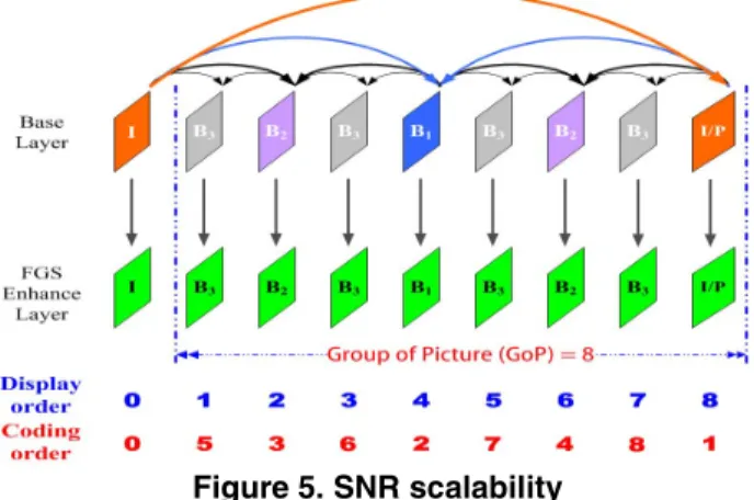
SNR scalability supports fine grain scalability, in which SNR enhancement layer (so-called PR slice) represents a refinement to the residual signal and can be truncated at any arbitrary point. The values of quantization parameter (QP) for base layer and SNR enhancement layer are different (QP increase of 6). In this paper, we focus on combined temporal and fine grain SNR scalability (FGS).

Figure 5. SNR scalability

There are some introduction works in [9-11]. The scalability of the SVC bitstream is modeled as a tree structure as shown in [7] (also see Figure 5). The edge between the nodes indicates that the scalability level is selected or not.

3. IEEE 802.11e MAC protocol

Because the demands of multimedia applications over IEEE 802.11 based WLANs increase tremendously in recent years, task group E of IEEE 802.11 proposed a QoS extension of the IEEE 802.11 standard in 2005, called 802.11e. EDCA is designed to provide prioritized QoS by enhancing the contention-based DCF. Before entering the MAC layer, each packet received from the higher layer is

242 242

(15)

assigned a specific user priority value and the priority value is tagged for each packet later. At MAC layer, EDCA introduces four different first-in first-out queues, called access categories (ACs). Each packet from the higher layer along with a specified user priority value should be mapped into a corresponding AC according to the type of traffic (e.g., background, best effort, video and voice). Each AC is also referred to as a backoff entity, which has its own contention parameters such as CWmin[AC], CWmax[AC], AIFS[AC]

(see equation(1)). Different contention parameters let different queues have different priorities and high priority queues can get more transmissions than low priority queues.

AIFS[AC] = SIFS + AIFSN[AC] * slot time, (1) where SIFS represents Short Interframe Space and AIFSN[AC] ≥ 2.

4. The proposed cross-layer architecture

In this section, based on the idea proposed in [12], we propose a cross-layer architecture for SVC transmission, enabling interaction between application layer (H.264/SVC codec) and MAC layer (IEEE 802.11e). The proposed cross- layer architecture is shown in Figure 6 and can ensure inter- QoS between H.264/SVC layers (VCL, NAL) and IEEE 802.11e MAC layer by the mapping algorithm.

Figure 6. The proposed cross-layer architecture The SVC VCL transforms video frames into base layer and enhance layer (FGS layer, also called progressive refinement). As a result, we obtain six kinds of slices: I, P,

B1, B2, B3 and PR. Each slice is sent to NAL which is the interface between VCL and the lower system layer.

Figure 7. SVC NAL unit header [13]

The size of SVC NAL unit header (as shown in Figure 7) is four bytes, where

- Byte 1 contains Forbidden Field (F), NAL unit Reference Indicator (NRI) and NAL unit type (TYPE).

- Byte 2 contains Reserved Bits (RR) and Simple Priority (PRID).

- Byte 3 represents Temporal (TL), Spatial (DID) and Quality level (QL).

- Byte 4 contains Layer Base Flag (B), Use Base Prediction Flag (U), Discardable Flag (D), Fragmented Flag (G), Last Fragment Flag (L), Fragment Order (FO) and Extension Flag (E).

As shown in Figure 5, base layer slice has higher importance than enhancement layer slice because the lower temporal level has greater influence on decoding [14]. So, we conclude the priority for these slices as shown in Table 1.

Slice Type TL Priority I, P 000 3

B₁ 001

2

B₂ 010

B₃ 011

PR

000 001 1 010 011

Table 1. The priority of slice

In order to ensure a cross layer QoS mapping, the choice of the AC is based on the influence level of decoding [15]. Thus, the packets of base layer slices (I/P) which are non-discardable and non-truncatable are mapped onto the highest access category AC2. Because the video quality is very sensitive to packet loss of the base layer slices, it is necessary to guarantee a bounded delay and minimal loss rate for the base layer slices. Furthermore, in order to ensure the quality of video, we map every slice’s PR (except B3) onto AC1. Finally, B3’s PR slice has little effect to the

243 243

(16)

playback quality, they are mapped onto lowest priority access category AC0.

TL DID QL Access Category

000 000 00

001,010,011 000 00 2 000,001,010 000 01 1

011 000 01 0

Table 2. Mapping algorithm

5. Simulations and results

In order to verify the performance of our proposed cross-layer architecture, we have conducted simulations with Qualnet 4.0 [16], as shown in Figure 8. The proposed architecture is compared to EDCA [12] (all SVC slices share the same AC). As shown in Figure 8, we combine the scalable CODEC (JSVM 8.0) with network simulator (Qualnet 4.0).

Figure 8. Simulation methodology

At first, we set the encoder’s configure file (as shown in Table 3) to generate SVC bitstreams (bit rate = 911.36 kbps).

And then, we use Bit Stream Extractor to transform SVC bitstream into packet trace. This packet trace can provide us some useful information, such as start position, packet length, Lid, Tid, Qid, Type, discardable and truncatable.

Input YUV foreman Frame number 300

Resolution CIF (352x288) Frame rate 30 (fps)

GOP 8 Intra period 24

Base layer QP 30 FGS layer(s) 1

Table 3. Encoder’s configure file

We conduct the simulations of unicasting H.264/SVC video transmission (from the server to a client) over IEEE 802.11b PHY (2 Mbps). Besides the H.264/SVC stream, the server station also generates background traffic (300 kbps) to the client to increase the virtual collisions at the server’s MAC

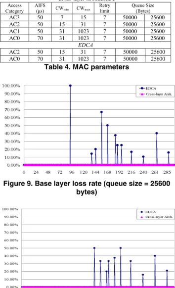
layer. Furthermore, we include four more stations in which two stations each generates 300 kbps of data using CBR traffic to the corresponding station in order to overload the wireless networks. Table 4 shows the MAC parameters used for the simulations.

Cross-layer Architecture Access

Category AIFS

(μs) CWmin CWmax Retry

limit Queue Size (Bytes)

AC3 50 7 15 7 50000 25600 AC2 50 15 31 7 50000 25600 AC1 50 31 1023 7 50000 25600 AC0 70 31 1023 7 50000 25600

EDCA

AC2 50 15 31 7 50000 25600 AC0 70 31 1023 7 50000 25600

Table 4. MAC parameters

Figure 9. Base layer loss rate (queue size = 25600 bytes)

Figure 10. Base layer loss rate (queue size = 50000 bytes)

Figures 9 and 10 show base layer’s packet lose rate in different queue sizes (25600 bytes and 50000 bytes) with cross-layer architecture and EDCA. The cross-layer architecture achieves no packet loss, but EDCA performs poorly. This is mainly due to the fact that our cross-layer architecture associates base layer’s packets with the access category AC2 that gives more channel access opportunities.

In contrast, EDCA lets base layer’s packets share the same queue with enhance layer’s packets. This leads to filling the

244 244

(17)

queue very quickly, resulting in high probability of dropping incoming packets.

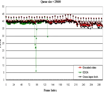
Figure 11. Objective video quality measurements (queue size = 25600 bytes)

Figure 12. Objective video quality measurements (queue size = 50000 bytes)

The phrase peak signal-to-noise ratio, often abbreviated PSNR, is an engineering term for the ratio between the maximum possible power of a signal and the power of corrupting noise that affects the fidelity of its representation. PSNR is employed as an objective video quality metric of our experiments. Figures 11 and 12 show the objective quality measurements of reconstructed video

streams in different queue sizes under two schemes (EDCA and cross-layer architecture). It is clearly seen that our architecture achieves smoother video quality degradation than EDCA. This result came up to our expectations, because of no packet loss of base layer. Further, it is interesting to note that we experienced the packet loss of 92^th and 144^th slices of base layer that can not be decoded successfully when transmitting video with EDCA [17, 18].

In contrast, in our architecture we are able to decode the whole video sequence (300 frames).

In order to prove that the simulation of our cross-layer architecture is in steady state, we duplicate foreman pictures six times (288 x 6 =1728 frames) as input video. Figure 12 shows that the proposed approach performs the same for every foreman duplications.

Figure 13. Objective video quality measurements (1728 frames)

6. Conclusions

In this paper we introduce a novel cross layer architecture for H.264/SVC video transmission over IEEE 802.11e WLANs. By enabling interaction between Network Abstraction Layer (NAL) and IEEE 802.11e MAC layer, our approach can provide differentiated services for base layer and enhance layers. The proposed mapping algorithm can take into account the characteristics of hierarchical encoding of the H.264/SVC such that the video stream can be decoded successfully. The simulation results show that our approach provides better video quality than the previous approach (EDCA).

7. References

[1] IEEE Std. 802.11g 2003, Part 11: Wireless LAN Medium Access Control (MAC) and Physical Layer (PHY) Specifications, Supp. IEEE Std. 802.11g, 2003.

245 245

(18)

[2] Draft Std. 802.11n, Part 11: Wireless LAN Medium Access Control (MAC) and Physical Layer (PHY) Specifications: Amendment: Enhancements for Higher Throughput, IEEE Draft Std. P802.11n/D2.00, Feb.

2007.

[3] IEEE Std. 802.11e-2005, Part 11: Wireless LAN Medium Access Control (MAC) and Physical Layer (PHY) Specifications. Amendment 8: Medium Access Control (MAC) Quality of Service Enhancements, IEEE Std 802.11e, Sep. 2005.

[4] ITU-T and ISO/IEC JTC 1, “Advanced Video Coding for Generic Audiovisual Services”, ITU-T Recommendation H.264 and ISO/IEC 14496-10 (MPEG4-AVC), Version 1: May 2003, Version 2: Jan.

2004, Version 3: Sep. 2004, Version 4: July 2005.

[5] ITU-T and ISO/IEC JTC 1, “Generic Coding of Moving Pictures and Associated Audio Information – Part 2: Video”, ITU-T Recommendation H.262 and ISO/IEC 13818-2 (MPEG-2 Video), Nov. 1994.

[6] J. Golston, D. Member, and A. Rao, “Video Compression: System Trade-Offs with H.264, VC-1 and Other Advanced CODECs”, TEXAS INSTRUMENTS White Paper, Aug.2006.

[7] JSVM 8 Reference Software, JVT-U202, Hangzhou, China, Oct. 2006.

[8] T. Wiegand, G. Sullivan, J. Reichel, H. Schwarz, and M. Wien (eds.), “Joint Draft 9 of SVC Amendment”, Marrakech, Morocco, Jan. 2007.

[9] H. Schwarz, D. Marpe, and T. Wiegand, “SNR- Scalable Extension of H.264/AVC”, IEEE ICIP 2004, Singapore, Oct. 2004.

[10] H. Schwarz, D. Marpe, T. Schierl, and T. Wiegand,

“Combined Scalability Support for the Scalable Extension of H.264/AVC”, IEEE ICME 2005, Amsterdam, The Netherlands, July 2005.

[11] H. Schwarz, D. Marpe, and T. Wiegand, “Overview of the Scalable H.264/MPEG4-AVC Extension”, IEEE ICIP 2006, Atlanta, GA, USA, Oct. 2006.

[12] A. Ksentini, M. Naimi, and A. Gueroui, “Toward an Improvement of H.264 Video Transmission over IEEE 802.11e through a Cross-layer Architecture”, IEEE Communications Magazine, Vol. 44, no. 1, pp. 107- 114, 2006.

[13] Y. K. Wang, M. M. Hannuksela, S. Pateux, and A.

Eleftheriadis, “System and Transport Interface of Emerging SVC Standard,” Joint Video Team (JVT), Doc. JVT-U151, Hangzhou, China, Oct. 2006.

[14] H. C. Huang, W. H. Peng, T. Chiang, and H. M. Hang,

“Advances in the scalable amendment of H.264/AVC,” IEEE Communications Magazine, Vol.

45, Iss. 1, pp. 68-76, Jan. 2007.

[15] K. Xu, Quanhong Wang, and H. Hassanein,

“Performance analysis of differentiated QoS supported by IEEE 802.11e enhanced distributed coordination function (EDCF) in WLANs,” Global

Telecommunications Conference, 2003. IEEE, Vol.2, Iss., 1-5, pp. 1048-1053, Dec. 2003.

[16] Qualnet 4.0. http://www.scalable-networks.com.

[17] A. Ksentini, M. Naimi, and A. Gueroui, “Toward an Improvement of H.264 Video Transmission over IEEE 802.11e through a Cross-layer Architecture”, IEEE Communications Magazine, Vol. 44, no. 1, pp. 107- 114, 2006.

[18] A. Ksentini, A. Gueroui, and M. Naimi, “Improving H.264 Video Transmission in 802.11e EDCA”, IEEE ICCCN 2005, San Diego, USA 2005.

246 246

無線感測網路中跳躍數導向位置估算演算法之研究

行政院國家科學委員會專題研究計畫 成果報告

行政院國家科學委員會專題研究計畫成果報告

A Hop-Oriented Position Estimation Algorithm for Wireless Sensor Networks

行政院國家科學委員會專題研究計畫成果報告