具狀態時延與時變干擾的非線性程序控制

行政院國家科學委員會專題研究計畫 成果報告

具狀態時延與時變干擾的非線性程序控制

計畫類別： 個別型計畫

計畫編號： NSC93-2214-E-011-009-

執行期間： 93 年 08 月 01 日至 94 年 07 月 31 日 執行單位： 國立臺灣科技大學化學工程系

計畫主持人： 周宜雄

計畫參與人員： 紀昆村

報告類型： 精簡報告

處理方式： 本計畫涉及專利或其他智慧財產權，1 年後可公開查詢

中 華 民 國 94 年 11 月 3 日

Process Control of Nonlinear State-Delayed Systems with Time-Varying Uncertainties

Yi-Shyong Chou

^∗

& Kuen-Tsuen Jih Department of Chemical Engineering

National Taiwan University of Science & Technology (NSC93-2214-E-011-009)

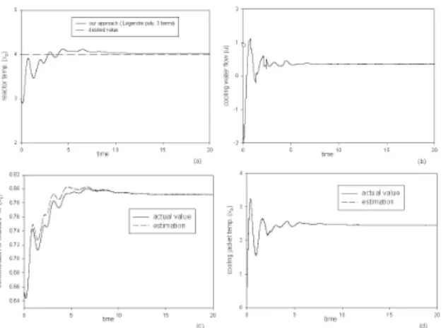
In this paper the problem of designing a tracking controller for uncertain nonlinear state- delay systems which can suppress the effects of both unknown uncertainties and disturbances is investigated. The controller is designed by using the sliding mode control concept and the polynomial approximation method. One of the features in this paper is that model uncertainties and state-delay terms are expressed as the Legendre polynomials expansion. The expansion coefficients of the Legendre polynomials can furthermore be modified by the update law derived from the Lyapunov stability theorem. The major advantage of the proposed control system design is to track a set-point without producing a vigorous control action and requiring the exact knowledge of model uncertainties. The control scheme is illustrated by an example of a chemical reactor with delayed states. Simulation results indicate that the proposed method can work for processes with time delays, in spite of unknown modeling uncertainties.

Keywords: uncertain nonlinear time-delay system, sliding mode control, chemical reactor con- trol

1. Introduction

Recently, control of nonlinear systems with unknown uncertainties has been of a challenging problem. Slo- tine and Coetsee (Slotine and Coetsee, 1986) proposed an adaptive sliding control to reduce the effect of un- certainties on the process for further improving perfor- mance by on-line parameter estimation algorithms. In their study, bounds of the unknown parameters did not need to be known. Huang and Kuo (Huang and Kuo, 2001) presented a sliding control scheme for nonlinear processes with unknown bound time-varying uncertain- ties. Those uncertainties were represented in finite-term Fourier functions. Vecchio et al. (Vecchio et al., 2002) developed a repeatable control design method for a class of feedback linearizable processes with an unknown non- linear function. They used the Fourier series to approxi- mate the nonlinear function of the process. In the above papers all uncertain elements appeared in the process were lumped and expanded in finite-term Fourier func- tions. This makes that we need choose a sufficiently large terms of Fourier functions to approximate uncer- tainties.

The aim of this paper is to design a sliding controller for nonlinear state-delay processes with time-varying un- certainties, despite unknown magnitudes on time delays and model uncertainties. The key idea of the paper is to use orthogonal polynomials to represent model un- certainties and delayed states. Due to the fact that the convergence of orthogonal polynomials is fast, only few terms of coefficients is needed to calculate. This allows us to improve the transient performance. Once the un-

known uncertainties and unknown state-delay terms have been approximated and parameterized, a feedback con- trol law and an update law for adjusting the parame- ters of orthogonal polynomials can be designed using the Lyapunov stability theory. The sliding mode con- trol structure is the backbone of the development of the proposed control strategy. The presented composite non- linear controller, which consists of a sliding model con- troller with a coefficient update law, can achieve offset- free performance. Furthermore, we discuss the stability of the closed-loop process. Finally effectiveness of the proposed method is demonstrated by illustrative simula- tions.

2. Problem Formulation

Consider a class of dynamic processes that may be modeled by

x

⁽ⁿ⁾

= f

t

(X(t), X(t − τ ))

+g

t

(X(t), X(t − τ ))u(t) + d(t) (1) where X = £

x x

⁽¹⁾

· · · x

⁽ⁿ⁻¹⁾

¤

T

is the process state vector, f

_t

and g

_t

are nonlinear functions, τ > 0 is a delay time in the process state, u is the control input, and d is the disturbance. Generally, a large class of chemi- cal processes can be represented with this type of model structures. Examples are like recycled reactors, recycled storage tanks, cold rolling mills and so on (?). Most of the recycling processes inherit delays in their state equa- tions. Equation 1 also can be expressed in companion

1

form, i.e.

˙x

1

= x

2

˙x

2

= x

3

.. .

˙x

n

= f

t

(X(t), X(t − τ ))

+g

t

(X(t), X(t − τ ))u(t) + d(t) (2) The control objective is to design a control law u(t) to make x(t) track x

d

(t) in the presence of unknown mod- eling errors in f

t

(X(t), X(x − τ )) and g

t

(X(t), X(t − τ )) and unknown disturbances, d(t).

The sliding mode design approach consists of two components. The first involves the design of a switching function so that the sliding motion satisfies design spec- ifications. The second is concerned with the selection of a control law which will make the switching function attractive to the system state. Thus, the first step is to define a time-varying surface s(t) in the state-space as s(X; t) = 0 that is a differential operator acting on some error function

s = µ d

dt + λ

¶

_n−1

e(t) (3)

e(t) = x(t) − x

d

(t) (4) where x

_d

(t) is the desired trajectory and λ is a strictly positive constant, determining the performance of the system on the sliding surface. The control goal is to force the process state x(t) to follow the specified tra- jectory x

_d

(t). The problem is equal to design a control law u(t) to ensure

t→∞

lim e(t) = 0 (5)

This condition can be achieved by requiring the system trajectory to converge to the sliding surface. Thus, the problem of tracking trajectory can be reduced to that of keeping s at zero.

µ d dt + λ

¶

_n−1

e(t) = 0 (6)

3 Controller Design

The first step in controller design is to select a feed- back control law u(t). The goal is to reach the slid- ing surface and to remain on it. The second step is to estimate unknown functions in f

_t

(X(t), X(t − τ )) and g

t

(X(t), X(t − τ )) by employing orthogonal polynomi- als. Classical orthogonal polynomials serve as an ex- cellent tool for modeling processes in an approximative way. Here we select the Legendre polynomials in order to improve the accuracy of approximation of unknown functions.

Recall eq 3 s =

µ d dt + λ

¶

_n−1

e(t) (7)

The derivative of the sliding surface is calculated as fol- lows:

˙s = x

⁽ⁿ⁾

− x

⁽ⁿ⁾_d

+ Ω(e) (8) where

Ω(e) =

n−1

X

k=1

(n − 1)!λ

^n−k

(n − k)!(k − 1)! e

^(k)

(9) Here we assume that the functions f

t

(X(t), X(t − τ )) and g

t

(X(t), X(t − τ )) can be represented as (?)

f

t

(X(t), X(t − τ )) = f (X(t))

+∆f (X(t), X(t − τ ))(10) g

t

(X(t), X(t − τ )) = g(X(t))

×∆g(X(t), X(t − τ ))(11) This assumption decomposes f

_t

(X(t), X(t − τ )) and g

t

(X(t), X(t − τ )) respectively into two parts, where f (X(t)) and g(X(t)) are referred to as the known func- tions whereas ∆f (X(t), X(t−τ )) and ∆g(X(t), X(t−

τ )) can be viewed as the time-varying uncertainties which are unknown functions of time. Here ∆g(X(t), X(t − τ )) is in general referred to as the matched uncertainty, which is known to be bounded as below:

∆g

min

≤ ∆g(X(t), X(t − τ )) ≤ ∆g

max

(12)

∆f (X(t), X(t − τ )) can be viewed as the mismatched uncertainty.

With the aid of eqs 10 and 11, substituting eq 1 into eq 8 obtains

˙s = (f + ∆F ) + g∆gu − x

⁽ⁿ⁾_d

+ Ω(e) (13) where ∆F = ∆f + d. In order to make the value of ˙s equal to zero, we consider the following control input of the form

u = 1

g h

− ∆ ˆ H

−∆ˆ g

⁻¹

(f − x

⁽ⁿ⁾_d

+ Ω(e)) − ηsat( s φ )

i (14) The thickness of the boundary layer φ is defined to be a positive real scalar. Outside the boundary layer, |s| ≥ φ, the sliding condition will be used to specify the s dynam- ics. Inside the boundary layer, |s| < φ, the control law will be modified to impose a smoothing process to the s dynamics. The tuning gain η is a strictly positive con- stant, ∆ ˆ H and ∆ˆ g

⁻¹

are the estimates of the unknown functions ∆F ∆g

⁻¹

and ∆g

⁻¹

, respectively. The sat is the saturation function

sat ³ s φ

´

=

½

_s

φ

if |

^s_φ

| < 1

sgn(

_φ^s

) if |

^s_φ

| ≥ 1 (15)

sgn ³ s φ

´

=

½ +1 if

_φ^s

> 0

-1 if

_φ^s

< 0 (16)

Substituting eq 14 into eq 13 gives

˙s = ∆g h

(f − x

⁽ⁿ⁾_d

+ Ω(e))(∆g

⁻¹

− ∆ˆ g

⁻¹

) +(∆H − ∆ ˆ H) − ηsat( s

φ ) i

(17) where

∆H = ∆F ∆g

⁻¹

(18)

Assume that ∆H and ∆g

⁻¹

are unknown bounded func- tions and can be approximated as

∆H ≈ W

_H^T

z

F

(t) (19)

∆g

⁻¹

≈ W

_g^T

z

F

(t) (20) where

z

F

(t) = £

P

0

(t) P

1

(t) · · · P

n

(t) ¤

_T

(21) W

H

= £

w

H0

w

H1

· · · w

Hn

¤

_T

(22) W

g

= £

w

g0

w

g1

· · · w

gn

¤

_T

(23) Here z

_F

is the Legendre polynomials vector, W

_H

and W

g

are the parameter vectors and considered as constant vectors. Generally the number n should be properly se- lected so that the approximate errors are tolerable. ∆ ˆ H and ∆ˆ g

⁻¹

are the estimates of the unknown functions

∆H and ∆g

⁻¹

, respectively, and can be represented as

∆ ˆ H ≈ W ˆ

_H^T

z

F

(t) (24)

∆ˆ g

⁻¹

≈ W ˆ

_g^T

z

F

(t) (25) where

W ˆ

H

= £ ˆ

w

H0

w ˆ

H1

· · · w ˆ

Hn

¤

_T

(26) W ˆ

g

= £

ˆ

w

g0

w ˆ

g1

· · · w ˆ

gn

¤

_T

(27) The update laws for adjusting the parameters ˆ W

H

and W ˆ

_g

will be derived.

Substituting eqs 19 to 27 into eq 17 yields

˙s = ∆g h

(f − x

⁽ⁿ⁾_d

+ Ω(e))( ˜ W

_g^T

z

F

(t)) + ˜ W

_H^T

z

F

(t) − ηsat( s

φ ) i

(28) where

W ˜

H

= W

H

− ˆ W

H

(29) W ˜

g

= W

g

− ˆ W

g

(30) Consider the Lyapunov function candidate as

V = 1

2 s

²

+ 1 2 ∆g h

W ˜

_H^T

Q

H

W ˜

H

+ ˜ W

_g^T

Q

g

W ˜

g

i (31) where Q

H

and Q

g

are symmetric positive definite matri- ces. The derivative of V along the trajectory is

V ˙ = s ˙s + ∆g

h W ˜

_H^T

Q

H

W ˜ ˙

H

+ ˜ W

_g^T

Q

g

W ˜ ˙

g

i

(32)

Since W

H

and W

g

are the constant vectors, W ˜ ˙

H

= − ˙ W ˆ

H

and W ˜ ˙

g

= − ˙ W ˆ

g

, the above equation can be further ex- pressed as

V ˙ = s ˙s + ∆g

h W ˜

_H^T

Q

H

(− ˙ W ˆ

H

)

+ ˜ W

_g^T

Q

_g

(− ˙ W ˆ

_g

) i

(33) Substituting eq 28 into 33 and considering within the boundary layer, we obtain

V ˙ = ∆g h

W ˜

_g^T

(z

F

s(f − x

⁽ⁿ⁾_d

+ Ω(e)) − Q

g

W ˆ ˙

g

)

+ ˜ W

_H^T

(z

F

s − Q

H

W ˆ ˙

H

) − η s

²

φ i

(34) Choose the update laws as

ˆ ˙

W

g

= Q

⁻¹_g

z

F

s(f − x

⁽ⁿ⁾_d

+ Ω(e)) (35) ˆ ˙

W

H

= Q

⁻¹_H

z

F

s (36)

then the derivative of V becomes V ˙ = −∆gη s

²

φ (37)

Choose η = |

_∆g^η1

max

|, η

1

> 0 Then V ˙ ≤ −η

1

s

²

φ ≤ 0 (38)

With the aid of the update laws eqs 35 and 36, the unknown functions, ∆H and ∆g, can be estimated and, consequently the control law eq 14 can be implemented.

4 Numerical Example

In this section, simulations of the control of an uncer- tain nonlinear time-delay system is performed using the proposed sliding control method. Consider the first or- der, irreversible, exothermic reaction A → B, carried out in a well mixed continuously stirred tank reactor.

Suppose that fresh feed of pure A is to be mixed with a recycled stream of unreacted A with recycle flow rate F

r

(1 − λ). If there is a delay, τ

r

, in the recycle stream, then the material and energy balance equations in dimen- sionless forms become

˙x

1

(t) = − 1

λ x

1

(t) + ( 1

λ − 1)x

1

(t − τ

s

) +D

a

(1 − x

1

(t)) exp n x

₂

(t)

1 +

^x2_ψ^(t)

o

(39)

˙x

2

(t) = − 1

λ x

2

(t) + ( 1

λ − 1)x

2

(t − τ

s

) +BD

a

(1 − x

1

(t)) exp n x

₂

(t)

1 +

^x2_ψ^(t)

o

−β

r

(x

2

(t) − x

3

(t)) (40)

˙x

3

(t) = β

c

(x

2

(t) − x

3

(t)) + u(x

3f

− x

3

(t))(41)

The main control objective for the reactor would be the regulation of the product concentration around a de- sired set-point value. The close relationship between the concentration of the component A and the temperature justifies choosing as the control objective the regulation of the reactor outlet temperature about a corresponding set-point value. The coolant flow-rate is considered here as the manipulated variable. Only the reactor tempera- ture x

2

is available. The observer for this reactor system must be designed to provide other state information. Fig- ure 1a shows the dynamic behavior of the process with a time-delay τ

_s

= 2 in the state in which the reference value of the dimensionless temperature x

₂

changes from x

2ss

= 3 to x

2

= 4. Figure 1b shows the input moves of the controller. The estimated states x

₁

and x

₃

of this sys- tem are depicted in Figure 1c and Figure 1d, respectively.

By comparing the estimated value and the real value, one can see that they present a very close behavior. Figure

Figure 1. (a). Process responses (b). Controller responses (c). Estimation result of x

₁

(d). Estima- tion result of x

3

2a presents the simulation results for the process with a time-delay τ

s

= 2 in the state under a set-point change from x

_2ss

= 3 to x

2

= 4 and an oscillatory disturbance d = 0.1 sin(t). In this case, the closed-loop performance remains satisfactory despite the extremely noisy nature of the time-varying disturbance. Figure 2b shows the in- put moves of the controller. Figures 2c and 2d present the estimated value and the real value of x

₁

and x

₃

, re- spectively. Figure 3a shows the simulation results for the process under a set-point change from x

_2ss

= 3 to x

2

= 4 and a time-delay τ

s

= 2 in the state for t ≤ 10, and a τ

s

= 5 in the state for t > 10. Figure 3b shows the input moves of the controller. As a whole, simulation re- sults show that satisfactory control performances can be obtained by applying this proposed strategy.

5 Conclusions

A control strategy to track a class of nonlinear state- delay systems with time-varying uncertainties is presented in this paper. Model uncertainties are represented as the expansion of the Legendre polynomials and are es-

Figure 2. (a). Process responses (b). Controller responses (c). Estimation result of x

₁

(d). Estima- tion result of x

₃

Figure 3. (a). Process responses (b). Controller responses

timated by updating the expansion coefficients. The pro- posed algorithm takes advantage of the fast convergence characteristics of the orthogonal polynomials. The closed- loop performance of the proposed controller is illustrated by numerical simulations. It is shown that the proposed method is able to track the desired trajectory despite time- varying modelling uncertainties.

6 Acknowledgement

The financial support of National Science Council (NSC) under Grant NSC 93-2214-E-011-009 is acknowl- edged.

References

Huang, A. C. and Y. S. Kuo (2001). Sliding control of nonlinear systems containing time-varying un- certainties with unknown bounds. Int. J. Control 74, 252–264.

Slotine, J. J. E. and J. A. Coetsee (1986). Adaptive slid- ing controller synthesis for nonlinear systems. Int.

J. Control 43, 1631–1651.

Vecchio, D. D., R. Marino and P. Tomei (2002). Adap-

tive state feedback control by orthogonal approx-

imation functions. Int. J. Adapt. Control Signal

Process. 16, 635–652.