拉瑪努江和於信號處理及週期偵測之應用

(1)

國立臺灣大學電機資訊學院電信工程學研究所博士論文

Graduate Institute of Communication Engineering College of Electrical Engineering and Computer Science

National Taiwan University Doctoral Dissertation

拉瑪努江和於信號處理及週期偵測之應用

Ramanujan’s Sum and Its Application to Signal Processing and Period Estimation

張國韋

Kuo-Wei Chang

指導教授：貝蘇章博士

Advisor: Soo-Chang Pei, Ph.D.

中華民國 107 年 5 月 May, 2018

(2)

(3)

誌謝

感謝真主，感謝我的父母，感謝貝老師，感謝中華電信的主管和同事們，感謝 530 實驗室的學長姐與學弟妹。這篇論文獻給所有幫助我的人。

(4)

(5)

Acknowledgements

Thanks everyone who supports me.

(6)

(7)

摘要

本論文利用拉瑪努江和 (Ramanujan’s sum) 的特性，舉出兩種信號處理上的應用。其一為建構零自相關的整數序列 (Integer zero autocorrleation sequence)，這在通訊系統上有廣泛的應用。他的原理是利用傅立葉轉換，把建構零自相關序列的數論問題，轉換成建構一個固定振幅信號 (constant amplitude) 的問題，這裡巧妙用上拉瑪努江和整數的特性。另一個應用是一維與二維的信號週期偵測。

利用拉瑪努江和週期以及整數的特性，週期信號可以被分解成一個個因數的週期，往後便可以針對不同的週期進行不同的處理，如同以前的濾波器組 (ﬁlter bank)。最後我們針對拉瑪努江和只能找出因數週期的缺點，採用全相位快速傅立葉 (all phase FFT) 演算法來改進。

全相位快速傅立葉演算法為利用相位的差，求出非整數的頻率，改進了以往頻率只能在整數上的缺點，可以幫助我們進行週期偵測。我們也順帶提到全相位快速傅立葉演算法的一些其他應用，包含唧聲信號 (chirp signal) 的頻率追蹤、快速二維頻率偵測等等。

(8)

(9)

Abstract

This thesis presents two applications of Ramanujan’s sum in the domain of signal processing. The ﬁrst one is integer zero autocorrelation sequence construction, which is useful in modern communication system. The concept is to transform this number theoretic problem into a constant amplitude signal construction problem, by Fourier transform and the integer property of Ramanujan’s sum. The second application is 1D and 2D period estimation. The periodic signal is separated into sub-period signals, just like ﬁlter bank. Each sub-period is a factor of the length. Finally we use all phase FFT to enhance the period estimation. All phase FFT use phase information to estimate frequency. The advantage is the frequency is non integer. Finally we propose some other applications of all phase FFT, such as chirp signal pitch tracking and fast 2D frequency estimation.

(10)

(11)

List of Figures

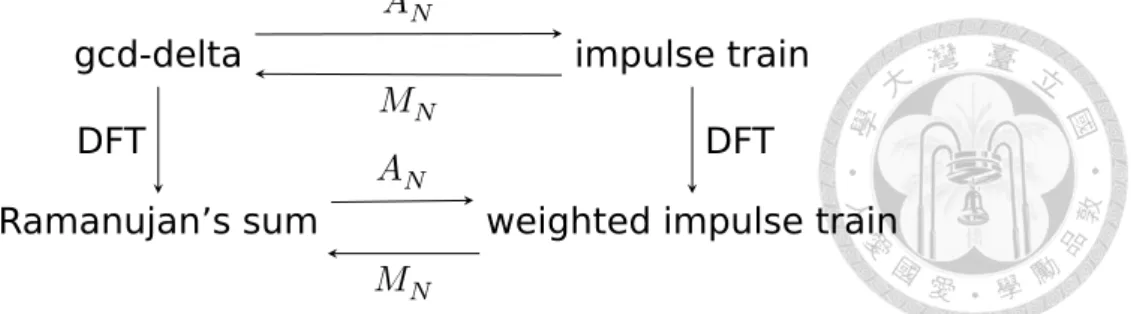
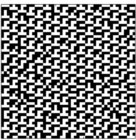
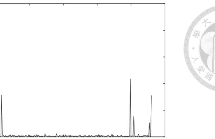
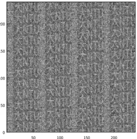
3.1 The spectrum of 𝑥, where 𝑥 is deﬁned in Equation (3.1). . . 28 3.2 Relations of gcd-delta, Ramanujan’s sum and impulse train 36 3.3 The original 2D Pattern . . . 57 3.4 Some random removal from Figure 3.3 . . . 57 3.5 Spectrum obtained from Figure 3.4 . . . 58 3.6 The image is a combination of Chinese characters and En-

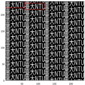
glish letters. The width is 60 pixels and the height is 20 pixels. The meaning of those two Chinese characters is National Taiwan University (NTU) . . . 60 3.7 The 240x240 image repeating the Figure 3.6. The period-

icity matrix is given in the text. The red box indicates the basic pattern and the direction of period . . . 60 3.8 A 240x240 noisy image with the pattern in Figure 3.6. The

added noise is white Gaussian with SNR=3db . . . 61 3.9 The spectrum from Figure 3.8. The ﬁrst peak (DC) is not

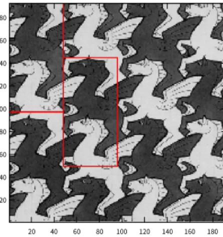
shown because the value is too large. . . 61 3.10Pegasus, by M.C. Escher 1959. The image is cropped and

downsampled to 192 × 192. The red box indicates the ap- proximated basic pattern. . . 63 3.11The spectrum from Figure 3.10. The ﬁrst peak (DC) is not

shown because the value is too large. . . 63

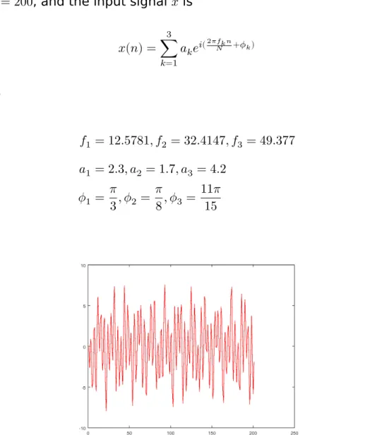
4.1 The real part of 𝑥 in Equation (4.8) . . . 74

(14)

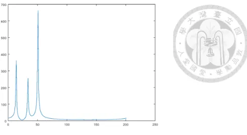
4.2 The power spectrum of 𝑥 in Equation (4.8), where window is not performed. . . 75 4.3 The power spectrum of 𝑥 in Equation (4.8), where window

is performed. . . 75 4.4 The step function with noise . . . 78 4.5 2D signal with two frequencies . . . 80 4.6 Signal with two chirp rate, represented in time-frequency

plane by all phase FFT. Red:𝛼₁ = 0.01,Blue:𝛼₂ = −0.01 Details are referred to the text. . . 82 4.7 Signal with two chirp rate, represented in time-frequency

plane by all phase FFT. Red:𝛼₁ = 0.1,Blue:𝛼₂ = −0.05. The red chirp is aﬀected when blue is near. . . 82 4.8 Absolute value of 𝑥, where 𝑥 is given in Equation (4.10),̂

𝑓 = 855.77. The decay is very fast near 850. . . 86

(15)

List of Tables

3.1 Similarity and diﬀerence between ideal ﬁlter and gcd-delta function . . . 29

(16)

(17)

Chapter 1 Introduction

1.1 Deﬁnition and Properties of Ramanujan’s Sum

A special sum of the roots of unity called Ramanujan’s sum[1]

𝑐_𝑞(𝑛) =

𝑞

∑

𝑎=1,(𝑎,𝑞)=1

𝑒^2𝜋𝑖^𝑎^𝑞^𝑛 (1.1)

where (𝑎, 𝑞) = 1 means that 𝑎 only takes on values coprime to 𝑞. For example,

𝑐₃(𝑛) = [2, −1, −1, 2, −1, −1, 2, −1, ...] (1.2) 𝑐₆(𝑛) = [2, 1, −1, −2, −1, 1, 2, 1, −1, ...] (1.3) 𝑐₇(𝑛) = [6, −1, −1, −1, −1, −1, −1, 6, −1, −1, ...] (1.4)

The sums have many good properties. First of all, they are all integer.

This is amazing because the roots of unity are complex number. The summation over complex is in general also complex, but the Ramanu- jan’s Sum is real and more surprisingly, integer. Secondly, the sums are

(18)

periodic,

𝑐_𝑞(𝑛 + 𝑞) = 𝑐_𝑞(𝑛) (1.5)

Additionally, since 𝑐_𝑞(𝑛) is real, we have

𝑐_𝑞(𝑛) = 𝑐^∗_𝑞(𝑛) =

𝑞

∑

𝑎=1,(𝑎,𝑞)=1

𝑒^−2𝜋𝑖^𝑎^𝑞^𝑛 = 𝑐_𝑞(−𝑛) (1.6)

where 𝑥^∗ is the complex conjugate of 𝑥. In other words, 𝑐_𝑞 is an even function.

Moreover, when signal length 𝑁 is a multiple of 𝑞, Ramanujan’s sum can be viewed as discrete Fourier transform (DFT) of a binary sequence.

For instance, let 𝑁 = 6

⎡⎢

⎢⎢

⎣ 0 1 0 0 0 1

⎤⎥

⎥⎥

⎦

−−→DFT

⎡⎢

⎢⎢

⎣ 2 1

−1

−2

−1 1

⎤⎥

⎥⎥

⎦ ,

⎡⎢

⎢⎢

⎣ 0 0 1 0 1 0

⎤⎥

⎥⎥

⎦

−−→DFT

⎡⎢

⎢⎢

⎣ 2

−1

−1 2

−1

⎤⎥

⎥⎥

⎦

(1.7)

As we can see, 𝑐₆(𝑛) and 𝑐₃(𝑛), 𝑛 = 0, 1, ..., 5 are constructed by 6-point DFT. Furthermore, since the binary sequences are orthogonal, the Ra- manujan’s sum 𝑐₆ and 𝑐₃ are also orthogonal. In general, if 𝑞₁ and 𝑞₂ are two diﬀerent factors of 𝑁 , then 𝑐_𝑞₁(𝑛) and 𝑐_𝑞₂(𝑛), 𝑛 = 0, 1, ..., 𝑁 − 1 are orthogonal.

Based on those good properies, the Ramanujan’s sum can be further used in analyzing long period time sequences such as stock price, DNA and protein coding[2, 3, 4]. In this thesis, we will introduce two applications in signal processing. The ﬁrst is to construct integer zero autocorrelation sequences, and the second is period estimation. We

(19)

deﬁne some useful functions and notations in the next section.

1.2 Preliminary

Unless otherwise speciﬁed, any signal or sequence 𝑥 in this thesis is periodic with length 𝑁 , and the index is 𝑛 with module 𝑁 , 𝑛 = 0, 1, 2, ..., 𝑁 −1.

In other words, 𝑥(−𝑛) = 𝑥(𝑁 −𝑛) and 𝑥(𝑁 +𝑛) = 𝑥(𝑛). The discrete Fourier transform (DFT) of 𝑥 is deﬁned as

̂

𝑥(𝑘) = 𝐹 {𝑥} =

𝑁−1

∑

𝑛=0

𝑥(𝑛)𝑊_𝑁^𝑛𝑘 (1.8)

where 𝑊_𝑁 = 𝑒^{−2𝜋𝑖/𝑁}, 𝑖 =√

−1. If there is no ambiguity, 𝑊 is used instead of 𝑊_𝑁 for convenience.

The delta function is

𝛿(𝑛) =

⎧{

⎨{

⎩

1 𝑛 = 0 0 otherwise

(1.9)

The autocorrelation of signal is deﬁned as

𝑅_𝑥𝑥(𝑘) =

𝑁−1

∑

𝑛=0

𝑥^∗(𝑛 − 𝑘)𝑥(𝑛) (1.10)

where 𝑥^∗ is the complex conjugate of 𝑥. And a signal 𝑥 is called zero- autocorrelation (ZAC) if 𝑅_𝑥𝑥(𝑘) = 𝐶𝛿(𝑘) for some nonzero constant 𝐶.

Some number theoretic deﬁnitions are given as follows. Let 𝑎 and 𝑏 be two integers, 𝑎|𝑏 means 𝑎 is a factor of 𝑏. The greatest common divisor (gcd) 𝑑 them is denoted as 𝑑 = gcd(𝑎, 𝑏) or simply 𝑑 = (𝑎, 𝑏). They are called coprime if (𝑎, 𝑏) = 1. The least common multiple of them is denoted as lcm(𝑎, 𝑏). The number in the form of 𝑎 + 𝑏𝑖 is called Gaussian integer. For a positive integer 𝑛, two integers 𝑎 and 𝑏 are said to be

(20)

congruent modulo 𝑛, written:

𝑎 ≡ 𝑏 (mod 𝑛) (1.11)

if their diﬀerence 𝑎 − 𝑏 is a multiple of 𝑛.

We deﬁne the set I_𝑘 = {𝑖|1 ≤ 𝑖 ≤ 𝑘, gcd(𝑖, 𝑘) = 1} to indicate all number between 1 and 𝑘 which is relatively prime to 𝑘.

2D signal is represented in capital letter like 𝑋, the default size is 𝑁 × 𝑁 and the index is given by 𝑋(𝑛₁, 𝑛₂). Two dimensional discrete Fourier transform (2DDFT) is deﬁned as

̂𝑋(𝑘₁, 𝑘₂) = ∑

𝑛₁

∑

𝑛₂

𝑋(𝑛₁, 𝑛₂)𝑊^𝑛¹^𝑘¹^+𝑛²^𝑘² (1.12)

(21)

Chapter 2 First Application: Integer and Gaussian Integer Zero

Autocorrelation Sequences

2.1 Motivation

Zero autocorrelation(ZAC) sequences have been extensively used in communication engineering, such as synchronization, CDMA [5, 6] and OFDM[7] system. They have also been applied to cryptography for constructing pseudo random sequences. In this work a special kind of ZAC sequences is considered, that is, integer ZAC (IZAC), because integer has the following advantages comparing to complex ﬂoating point number.

1) Integer requires less memory, for both saving and sending.

2) Arithmetic operations can be done faster and error-free.

3) The system can be implemented on hardware easily.

(22)

There are some trivial IZAC . The most obvious one is

⎛⎜

⎜⎜

⎝ 1 0 0

⋮ 0 0

⎞⎟

⎟⎟

⎠

The second one, although less known, is still in simple form

⎛⎜

⎜⎜

⎝

𝑁 − 2

−2

⋮

−2

⎞⎟

⎟⎟

⎠

where 𝑁 is the signal length. For example, 𝑁 = 5 and 𝑁 = 6

⎛⎜

⎜⎜

⎜

⎝ 3

−2

⎞⎟

⎟⎟

⎟

⎠ and

⎛⎜

⎜⎜

⎝ 4

−2

⎞⎟

⎟⎟

⎠

When 𝑁 is a composite number, constructing integer-valued ZAC from its factor by zero-padding is not diﬃcult to think of. Let say 𝑁 = 15 = 3×5, by the examples given above, we can organize signals like

(3, 0, 0, −2, 0, 0, −2, 0, 0, −2, 0, 0, −2, 0, 0)

(23)

or

(1, 0, 0, 0, 0, −2, 0, 0, 0, 0, −2, 0, 0, 0, 0)

One natural question is, are there any non-trivial integer-valued ZAC?

The answer is yes, such as

⎛⎜

⎜⎜

⎝ 2

−1

−1 2

−1 5

⎞⎟

⎟⎟

⎠

Similarly, non-trivial Gaussian integer ZAC can also be found. In the following, we will introduce how to construct those sequences.

2.2 Related Works

There are two types of construction method for IZAC. The ﬁrst type is solving equation directly. The other is by generating a constant amplitude (CA) sequence in frequency domain such that its discrete Fourier transform is integer. A constant amplitude sequence 𝑥(𝑛) is deﬁned as

|𝑥(𝑛)| = 𝐶 (2.1)

for some constant 𝐶. The reason behind the second method is by the following theorem.

Theorem 2.2.1. A sequence 𝑥 is CA if and only if its DFT 𝑥 is ZAC.̂ Similarly, a sequence 𝑥 is ZAC if and only if its DFT ̂𝑥 is CA.

Proof. See [8]

(24)

For convenience, we call the ﬁrst method time domain method and the other frequency domain method. As we will see, time domain meth- ods usually have to deal with non-linear equations, while frequency domain methods have to guarantee its DFT is integer. Both of them have some issues to conquer, but frequency domain methods are more sys- tematic and easier to solve.

2.2.1 Time domain method I: Making extra constraints

Consider 𝑁 = 5, the construction of IZAC is solving a ﬁve-variable equation.

𝑥(0)𝑥(1) + 𝑥(1)𝑥(2) + 𝑥(2)𝑥(3) + 𝑥(3)𝑥(4) + 𝑥(4)𝑥(0) = 0 (2.2) 𝑥(0)𝑥(2) + 𝑥(1)𝑥(3) + 𝑥(2)𝑥(4) + 𝑥(3)𝑥(0) + 𝑥(4)𝑥(1) = 0 (2.3) 𝑥(0)𝑥(3) + 𝑥(1)𝑥(4) + 𝑥(2)𝑥(0) + 𝑥(3)𝑥(1) + 𝑥(4)𝑥(2) = 0 (2.4) 𝑥(0)𝑥(4) + 𝑥(1)𝑥(0) + 𝑥(2)𝑥(1) + 𝑥(3)𝑥(2) + 𝑥(4)𝑥(3) = 0 (2.5)

where 𝑥(𝑛) ∈ ℤ. We can notice that eq. (2.4) is equivalent to eq. (2.3) and eq. (2.5) is equivalent to eq. (2.2). Thus, there are actually only two non-linear equations here. To solve this directly seems impossible, an alternative way is making more constraints. In particular, let 𝑥(0) = 𝑥(1) = 1, eq. (2.2) and eq. (2.3) become

1 + 𝑥(2) + 𝑥(2)𝑥(3) + 𝑥(3)𝑥(4) + 𝑥(4) = 0 (2.6) 𝑥(2) + 𝑥(3) + 𝑥(2)𝑥(4) + 𝑥(3) + 𝑥(4) = 0 (2.7)

Let 𝑥(3) = 𝑎 we can ﬁnd

𝑥(2) + 𝑥(4) = −1

𝑎 + 1 (2.8)

𝑥(2)𝑥(4) = −2𝑎 + 1

𝑎 + 1 (2.9)

(25)

⇒ (𝑥(2) − 𝑥(4))² = 1

(𝑎 + 1)² + 8𝑎 − 4 𝑎 + 1

= 8𝑎³+ 16𝑎²+ 4𝑎 − 3

(𝑎 + 1)² (2.10)

Since 𝑥(2), 𝑥(3) = 𝑎, and 𝑥(4) are all rational (which can be modiﬁed into integer easily by multiplying the denominators), eq. (2.10) means there are two rational numbers 𝑦 and 𝑎, where 𝑦 = (𝑥(2) − 𝑥(4))(𝑎 + 1), such that

𝑦² = 8𝑎³+ 16𝑎²+ 4𝑎 − 3

This is exactly a well-known rational Elliptic Curves problem[9, 10]. El- lipitic Curves problem has been studied a lot for the past few decades, and its main application is cryptography[11]. In short, if there are two non-trivial rational points (𝑦, 𝑎) on the Elliptic curve, then there are in- ﬁnite rational points on it [9]. In this case, since we already know the answer [−3, 2, 2, 2, 2] is integer ZAC, so when 𝑥(0) = 𝑥(1) = 1, 𝑥(3) = 𝑎 has two choices 1, −3/2. By ﬁnding the next point we can get 𝑎 = −7/8 and the new integer ZAC is

[8, 8, −12, −7, −52]

and the next is

[22, 22, 142, 462, −143]

and so on.

In general, making extra constraints can reduce the problem, and we have found a interesting connection to elliptic curve. However, the method is ad hoc and diﬃcult to ﬁnd a solution for arbitrary 𝑁 .

2.2.2 Time domain method II:Linear equation method

Another way to generate ZAC is given in [12]. This method only works for Gaussian integer and signal length 𝑁 = 𝑝^𝑘where 𝑝 is a prime number.

(26)

It also reduces the problem by making more constraints. In the following we summarize this method by setting 𝑁 = 9.

The ﬁrst constraint is called grouping. The index 𝑛 = 0, 1, 2, ..., 𝑁 − 1 is divided into several groups, and 𝑥(𝑛) is the same if 𝑛 is in the same group. For 𝑁 = 9, we have 3 groups

𝑥(0) (2.11)

𝑥(3) = 𝑥(6) (2.12)

𝑥(1) = 𝑥(2) = 𝑥(4) = 𝑥(5) = 𝑥(7) = 𝑥(8) (2.13)

One can notice that the index 𝑛 is divided by gcd(𝑛, 𝑁 ). In other words, if gcd(𝑛₁, 𝑁 ) = gcd(𝑛₂, 𝑁 ), then 𝑛₁ and 𝑛₂ are in the same group. The varibles in this problem is reduced from 9 to 3. Moreover, the number of equations for ZAC is reduced into 2.

𝑥^∗[0]𝑥(1) + 𝑥^∗(1)𝑥(0) + 3|𝑥(1)|²+ 2(𝑥^∗(3)𝑥(1) + 𝑥^∗(1)𝑥(3)) = 0 (2.14) 𝑥^∗[0]𝑥(3) + |𝑥(3)|²+ 𝑥^∗(3)𝑥(0) + 6|𝑥(1)|² = 0 (2.15)

Since 𝑥 is Gaussian integer, let 𝑥(𝑛) = 𝑥_𝑛+ 𝑖𝑦_𝑛 and rewrite the above

2(𝑥₀𝑥₁+ 𝑦₀𝑦₁) + 3(𝑥²₁+ 𝑦²₁) + 4(𝑥₁𝑥₃+ 𝑦₁𝑦₃) = 0 (2.16) 2(𝑥₀𝑥₃+ 𝑦₀𝑦₃) + (𝑥²₃+ 𝑦²₃) + 6(𝑥²₁+ 𝑦²₁) = 0 (2.17)

Next, Equation (2.17) subtracts Equation (2.16).

(𝑥₃− 𝑥₁)(2𝑥₀− 3𝑥₁+ 𝑥₃) + (𝑦₃− 𝑦₁)(2𝑦₀− 3𝑦₁+ 𝑦₃) = 0 (2.18)

Here comes the second constraint. Although Equation (2.18) is still a non-linear equation like Equation (2.2), we can use two linear equations

(27)

to approximate it.

𝑥₃− 𝑥₁ = −𝑦₃− 𝑦₁ (2.19)

2𝑥₀− 3𝑥₁+ 𝑥₃ = 2𝑦₀− 3𝑦₁+ 𝑦₃ (2.20)

Note that the equations above can only represent part of the solutions in Equation (2.18). For instance,

𝑥₃− 𝑥₁ = 6 (2.21)

2𝑥₀− 3𝑥₁+ 𝑥₃ = 2 (2.22)

𝑦₃− 𝑦₁ = −4 (2.23)

2𝑦₀− 3𝑦₁+ 𝑦₃ = 3 (2.24)

may be a solution of Equation (2.18), but it is not a solution of Equa- tions (2.19) and (2.20). To summarize, time domain methods face the non-linear equations directly. It is a hard problem without making extra constraints. In the following, we will introduce some frequency domain methods. By the Theorem 2.2.1, this number theoretic problem can be solved easily by Fourier transform.

2.2.3 Frequency domain method I:The Geometric se- quence method

The method in this section has been submitted to Eusipco 2018.

For any length 𝑁 , there are two trivial ZAC integer sequences[13]

𝑥(𝑛) = [1, 0, 0, 0, ..., 0] (2.25) 𝑥(𝑛) = [𝑁 − 2, −2, −2, −2, ..., −2] (2.26)

Moreover, if 𝑁 is even, the following sequence is also a ZAC integer

(28)

sequence.

𝑥(𝑛) =

⎧{

⎨{

⎩

𝑁−22 𝑛 = 0 (−1)^𝑛−1 𝑛 ≠ 0

(2.27)

Observe Equations (2.25) to (2.27), we can find two interest things. The first is that only the element 𝑥(0) is different from the others. The second is that each 𝑥(𝑛), 𝑛 ≠ 0 forms a geometric series. In Equation (2.25), [0, 0, ..., 0] can be viewed as geometric series with any ratio 𝑟. In Equa- tion (2.26), the ratio 𝑟 = 1 while in Equation (2.27), the ratio 𝑟 = −1.

Another example can be found in 𝑁 = 4. The closed form solution for perfect integer sequence is

[−𝑏, 𝑎, 𝑏,𝑏²

𝑎 ] (2.28)

where 𝑎, 𝑏,^𝑏_𝑎² are integers. This is solved by brute force. The last three terms [𝑎, 𝑏,^𝑏_𝑎²] can also be viewed as geometric series, with ratio 𝑟 = _𝑎^𝑏.

From the observation above, a natural assumption is that any geometric series can be used to generate perfect integer sequence. With some calculation the assumption can be proved. The result is given as follows. Let 𝑟 be an integer. A closed form perfect integer sequences is given as

𝑥(𝑛) =

⎧{

⎨{

⎩

−^𝑁−1∑

𝑘=2

𝑟^𝑘 𝑛 = 0 (1 + 𝑟)𝑟^𝑛 𝑛 ≠ 0

(2.29)

Note that 𝑥(𝑛) is a geometric series from 𝑛 = 1 to 𝑁 − 1. Since 𝑟 = 0 or 𝑟 = ±1 gives only trivial result, from now on only the cases 𝑟 ≠ 0, ±1 are discussed. For a concrete example, let 𝑁 = 5 and 𝑟 = 2

𝑥(𝑛) = [−(2²+ 2³+ 2⁴), 3 ⋅ 2¹, 3 ⋅ 2², 3 ⋅ 2³, 3 ⋅ 2⁴] (2.30)

= [−28, 6, 12, 24, 48] (2.31)

(29)

For another example, let 𝑁 = 6 and 𝑟 = −3

𝑥(𝑛) =

⎡⎢

⎢⎢

⎢

⎣

− ∑⁵_𝑘=2(−3)^𝑘 (−2) ⋅ (−3)¹ (−2) ⋅ (−3)² (−2) ⋅ (−3)³ (−2) ⋅ (−3)⁴ (−2) ⋅ (−3)⁵

⎤⎥

⎥⎥

⎥

⎦

(2.32)

= [180, 6, −18, 54, −162, 486] (2.33)

The two examples above illustrate that both prime length 𝑁 = 5 and composite length 𝑁 = 6 can be used. In fact, there is no limitation on signal length. To prove Equation (2.29), by Theorem 2.2.1 we should check that ̂𝑥 is CA. By deﬁnition,

̂

𝑥(𝑚) =

𝑁−1

∑

𝑛=0

𝑥(𝑛)𝑊_𝑁^𝑛𝑚 (2.34)

= −

𝑁−1

∑

𝑘=2

𝑟^𝑘+

𝑁−1

∑

𝑛=1

(1 + 𝑟)𝑟^𝑛𝑊_𝑁^𝑛𝑚 (2.35)

= (−

𝑁−1

∑

𝑘=2

𝑟^𝑘) − (1 + 𝑟) + (1 + 𝑟)

+ (1 + 𝑟)

𝑁−1

∑

𝑛=1

𝑟^𝑛𝑊_𝑁^𝑛𝑚 (2.36)

= −

𝑁−1

∑

𝑘=0

𝑟^𝑘+ (1 + 𝑟)

𝑁−1

∑

𝑛=0

𝑟^𝑛𝑊_𝑁^𝑛𝑚 (2.37)

= −1 − 𝑟^𝑁

1 − 𝑟 + (1 + 𝑟)1 − (𝑟𝑊_𝑁^𝑚)^𝑁

1 − 𝑟𝑊_𝑁^𝑚 (2.38)

= −1 − 𝑟^𝑁

1 − 𝑟 + (1 + 𝑟) 1 − 𝑟^𝑁

1 − 𝑟𝑊_𝑁^𝑚 (2.39)

= (1 + 𝑟)(1 − 𝑟^𝑁) ( 1

1 − 𝑟𝑊_𝑁^𝑚 − 1

1 − 𝑟²) (2.40)

To prove ̂𝑥 is CA, the following lemma is needed.

(30)

Lemma 2.2.2. For any complex number 𝑧 = 𝑟𝑒^𝑖𝜃, where 𝑟 = |𝑧| ≠ 1,

∣ 1

1 − 𝑧 − 1

1 − 𝑟²∣ = ∣ 𝑟

1 − 𝑟²∣ (2.41)

In other words, the magnitude of _1−𝑧¹ − _1−𝑟¹₂ only depends on 𝑟 and is independent from 𝜃.

Proof.

1

1 − 𝑟𝑒^𝑖𝜃 − 1

1 − 𝑟² = 1

1 − 𝑟 cos(𝜃) + 𝑖𝑟 sin(𝜃) − 1

1 − 𝑟² (2.42)

= 1 − 𝑟 cos(𝜃) − 𝑖𝑟 sin(𝜃)

(1 − 𝑟 cos(𝜃))²+ 𝑟²sin²(𝜃)− 1

1 − 𝑟² (2.43)

= ( 1 − 𝑟 cos(𝜃)

1 − 2𝑟 cos(𝜃) + 𝑟² − 1

1 − 𝑟²) − 𝑖 𝑟 sin(𝜃)

1 − 2𝑟 cos(𝜃) + 𝑟² (2.44)

Thus, let 𝑄 = 1 − 2𝑟 cos(𝜃) + 𝑟²

∣ 1

1 − 𝑟𝑒^𝑖𝜃 − 1 1 − 𝑟²∣

2

(2.45)

= (1 − 𝑟 cos(𝜃)

𝑄 − 1

1 − 𝑟²)

2

+ (𝑟 sin(𝜃)

𝑄 )

2

(2.46)

=(1 − 𝑟 cos(𝜃))²

𝑄² − 21 − 𝑟 cos(𝜃)

𝑄(1 − 𝑟²) + 1

(1 − 𝑟²)² +𝑟²sin²(𝜃)

𝑄² (2.47)

Note that (1 − 𝑟 cos(𝜃))²+ 𝑟²sin²(𝜃) = 𝑄

∣ 1

1 − 𝑟𝑒^𝑖𝜃 − 1 1 − 𝑟²∣

2

(2.48)

=𝑄

𝑄² − 21 − 𝑟 cos(𝜃)

𝑄(1 − 𝑟²) + 1

(1 − 𝑟²)² (2.49)

= 1 − 𝑟²

𝑄(1 − 𝑟²)− 21 − 𝑟 cos(𝜃)

𝑄(1 − 𝑟²) + 1

(1 − 𝑟²)² (2.50)

=−1 + 2𝑟 cos(𝜃) − 𝑟²

𝑄(1 − 𝑟²) + 1

(1 − 𝑟²)² (2.51)

= −𝑄

𝑄(1 − 𝑟²)+ 1

(1 − 𝑟²)² = 1 − (1 − 𝑟²)

(1 − 𝑟²)² = ( 𝑟 (1 − 𝑟²))

2

(2.52)

which completes the proof.

(31)

We can now prove 𝑥(𝑛) in Equation (2.29) is ZAC. By (2.40) and Lemma 2.2.2,

| ̂𝑥(𝑚)| = ∣(1 + 𝑟)(1 − 𝑟^𝑁) ( 1

1 − 𝑟𝑊_𝑁^𝑚 − 1

1 − 𝑟²)∣ (2.53)

= |(1 + 𝑟)(1 − 𝑟^𝑁)| ⋅ ∣ 1

1 − 𝑟𝑊_𝑁^𝑚 − 1

1 − 𝑟²∣ (2.54)

= ∣𝑟(1 + 𝑟)(1 − 𝑟^𝑁)

1 − 𝑟² ∣ = ∣𝑟(1 − 𝑟^𝑁)

1 − 𝑟 ∣ (2.55)

in other words, | ̂𝑥| is constant when 𝑟 is ﬁxed. Thus, 𝑥 is CA and bŷ Theorem 2.2.1, 𝑥 is ZAC.

This method looks like a time domain method, because the power series is used in time domain. However, the ZAC property is proved by Theorem 2.2.1, so it is actually a frequency domain method. This construction of ZAC works for Gaussian integer as well, by set 𝑟 = 𝑎 + 𝑏𝑖.

The main drawback of this method is that the dynamic range is too large. If 𝑟 = 2 and 𝑁 = 100, the max value of the ZAC sequence will be about 2¹⁰⁰ ≈ 10³⁰, although it is still integer.

2.2.4 Frequency domain method I:Legendre sequence method

The methods in this section have been published in [14].

Using Legendre sequence and Gauss sum when 𝑁 is prime

Recall that when 𝑁 is prime, Legendre symbol is deﬁned as

(𝑛 𝑁) =

⎧{ {

⎨{ {⎩

1, if 𝑛 ≡ 𝑥²(mod 𝑁 ), for some 𝑥 0, 𝑛 ≡ 0(mod 𝑁 )

−1, 𝑜𝑡ℎ𝑒𝑟𝑤𝑖𝑠𝑒.

(32)

And the Gauss sum is deﬁned as

𝐺(𝑘) =

𝑁−1

∑

𝑛=0

(𝑛

𝑁) 𝑒^{−2𝜋𝑖𝑘𝑛/𝑁}

A well known result[15] is that

𝐺(𝑘) =

⎧{

⎨{

⎩

(_𝑁^𝑘)√

𝑁 , 𝑁 ≡ 1(mod 4)

− (_𝑁^𝑘) 𝑖√

𝑁 , 𝑁 ≡ 3(mod 4)

In other words, the Fourier transform of Legendre Sequences is almost CA, with the only exception on 𝑘 = 0, the ﬁrst point. The amplitude is

√𝑁 thus our goal is to ﬁnd a Gaussian integer 𝑎 and some integers 𝑏, and 𝑐 such that

|𝑎|² = 𝑏²+ 𝑁 𝑐² (2.56)

Then a sequence that

𝑓(𝑛) =

⎧{

⎨{

⎩

𝑎, 𝑛 = 0

(_𝑁^𝑛)√

𝑁 𝑐 + 𝑏𝑖, 𝑛 ≠ 0

(2.57)

is CA, and the DFT of 𝑓(𝑛) is ZAC in Gaussian integer. Before we prove this let’s see some tiny examples of 𝑁 = 3 and 𝑁 = 5

Example 2.2.1. For 𝑁 = 3, the most trivial value we can choose is 𝑎 = 2, 𝑏 = 1,and 𝑐 = 1. Thus

𝑓(𝑛) = [2, 1𝑖 +√

3, 1𝑖 −√ 3}

̂𝑓(𝑘) = 𝐹 {𝑓(𝑛)} = {2 + 2𝑖, 2 − 4𝑖, 2 + 2𝑖]

As we can see, 𝑓(𝑛) is CA and 𝑓(𝑘) is with Gaussian integer value.̂ This example shows us 𝑎 does not necessary to be complex.

(33)

Example 2.2.2. N=3. Let’s try a non-trivial value c=2,b=5,a=6+1i

𝑓(𝑛) = [6 + 1𝑖, 5𝑖 + 2√

3, 5𝑖 − 2√ 3}

̂𝑓(𝑘) = {6 + 11𝑖, 6 − 10𝑖, 6 + 2𝑖]

From this example we can get a very diﬀerent result from the previous one. Note that 𝑎 has three alternatives 6 − 1𝑖, 1 + 6𝑖, and 1 − 6𝑖. They all give us diﬀerent ZAC sequences.

Example 2.2.3. 𝑁 = 5, 𝑐 = 1, 𝑏 = 0, 𝑎 = 2 + 1𝑖

𝑓(𝑛) = [2 + 1𝑖,√ 5, −√

5, −√ 5,√

5}

̂𝑓(𝑘) = {2 + 1𝑖, 7 + 1𝑖, −3 + 1𝑖, −3 + 1𝑖, 7 + 1𝑖]

There are various ways to construct infinite triples (𝑎, 𝑏, 𝑐) satisfied (2.56). Let 𝑎 = 𝑎_𝑟 + 𝑖𝑎_𝑖, where 𝑎_𝑟, 𝑎_𝑖 are integers. If we choose 𝑐 = 0, clearly the (2.56) will reduce to 𝑎²_𝑟+ 𝑎²_𝑖 = 𝑏², and it has infinite solutions.

If 𝑁 is odd, we can choose any odd 𝑐 and any even 𝑎_𝑟. Now (2.56) becomes

𝑎²_𝑟+ 𝑎²_𝑖 = 𝑏²+ 𝑁 𝑐²

⇒𝑎²_𝑖 − 𝑏² = 𝑁 𝑐²− 𝑎²_𝑟

Since 𝑁 and 𝑐 are odd and 𝑎_𝑟is even, 𝑁 𝑐²−𝑎²_𝑟 must be odd. Let 𝑁 𝑐²−𝑎²_𝑟= 2𝑘 + 1, then we can use 𝑎_𝑖 = 𝑘 + 1 and 𝑏 = 𝑘. Similarly, for any even 𝑐 and odd 𝑎_𝑟, we can ﬁnd proper 𝑎_𝑖 and 𝑏 by the same trick.

We complete this subsection by proving the claim that 𝑓(𝑘) is ZAĈ with Gaussian integer value.

Proof. Since 𝑓(𝑛) is CA by deﬁnition, thus𝑓(𝑘) is ZAC by Theorem 2.2.1.̂ To prove they are all Gaussian integer, we actually give 𝑓(𝑘) a closed̂

(34)

form. If 𝑁 ≡ 1(mod 4)

̂𝑓(𝑘) =

⎧{ {

⎨{ {⎩

𝑎 + (𝑁 − 1)𝑏𝑖, 𝑘 = 0

𝑎 + (_𝑁^𝑘) 𝑁 𝑐 − 𝑏𝑖, 𝑘 ≠ 0

If 𝑁 ≡ 3(mod 4)

̂𝑓(𝑘) =

⎧{ {

⎨{ {⎩

𝑎 + (𝑁 − 1)𝑏𝑖, 𝑘 = 0

𝑎 − (_𝑁^𝑘) 𝑁 𝑐𝑖 − 𝑏𝑖, 𝑘 ≠ 0

Either case the 𝑓(𝑘) is in Gaussian integer value since 𝑎 is Gaussian̂ integer and 𝑏, 𝑐 are integers.

Using GLS when 𝑁 is 4𝑘 + 1 prime

When 𝑁 is 4𝑘 + 1 prime, there is another way to increase the degree of freedom by using Generalized Legendre Sequences (GLS)[16, 17, 18]. GLS are originally applied to construct the eigenvectors of discrete Fourier transform (DFT) and generate a complete 𝑁 -dimensional orthogonal basis[18], because they have the property that their Fourier transform is their conjugate multiply a constant whose absolute value is √

𝑁 . All the values except the ﬁrst one of GLS lies on unit circle, and when 𝑁 = 4𝑘 + 1 we can choose the ones which only contains [1, 𝑖, −1, −𝑖], in order to bound the sequences in gaussian integer. The detail steps is described as follows:

1)Choose a GLS 𝑥 where the ﬁrst value is 0 and the rest only contain [1, 𝑖, −1, −𝑖].

2)Take DFT of 𝑥. Now we have a sequence 𝑦 that the ﬁrst value is still 0, but the absolute value of rest all equal to√

𝑁 .

3)The ﬁrst value of 𝑦 can then be chosen by a Gaussian integer 𝑎 + 𝑏𝑖 satisfying 𝑎² + 𝑏² = 𝑁 , which always exists by Fermat’s theorem. Now

(35)

the sequence is constant amplitude.

4) The DFT of y is a ZAC with Gaussian integer.

It is easy to prove this sequence is really in Gaussian integer. In fact, the sequence is actually

𝐹 {𝐹 {𝑥(𝑛)} + (𝑎 + 𝑏𝑖)𝛿(𝑛)} = 𝑁 𝑥(𝑁 − 𝑛) + 𝑎 + 𝑏𝑖

where 𝑁 , 𝑎, 𝑏, and all value in 𝑥 are with Gaussian integer, so will be the sequence.

As a concrete example, assume 𝑁 = 13 and we choose a GLS 𝑥

𝑥 = [0, 1, −𝑖, 1, −1, −𝑖, −𝑖, 𝑖, 𝑖, 1, −1, 𝑖, −1]

And we choose 𝑎 + 𝑏𝑖 = 3 + 2𝑖 since 3²+ 2² = 13. Thus the ZAC sequence is

𝑁 𝑥(𝑁 − 𝑛) + 𝑎 + 𝑏𝑖 =

13 [0, −1, 𝑖, −1, 1, 𝑖, 𝑖, −𝑖, −𝑖, −1, 1, −𝑖, 1] + 3 + 2𝑖

= [3 + 2𝑖, −10 + 2𝑖, 3 + 15𝑖, −10 + 2𝑖,

16 + 2𝑖, 3 + 15𝑖, 3 + 15𝑖, 3 − 11𝑖, 3 − 11𝑖, −10 + 2𝑖, 16 + 2𝑖, 3 − 11𝑖, 16 + 2𝑖]

This idea of this method can be extended by multiplying an integer or a Gaussian integer in step 2, and then we can have more choices in step 3. Let the length 𝑁 = 𝑎² + 𝑏², then we can ﬁnd an integer or a Gaussian integer 𝑠, satisfying |𝑠| = √

𝑐²+ 𝑑² with some integer 𝑐 and 𝑑, and multiply this number to the GLS. The choices in step 3 can be doubled because

(𝑎²+ 𝑏²)(𝑐²+ 𝑑²) = (𝑎𝑑 + 𝑏𝑐)²+ (𝑎𝑐 − 𝑏𝑑)² = (𝑎𝑑 − 𝑏𝑐)²+ (𝑎𝑐 + 𝑏𝑑)²

(36)

Thus by multiply diﬀerent 𝑐 + 𝑑𝑖 we can get diﬀerent ZAC sequences.

This gives us inﬁnite choices.

For instance, if 𝑁 = 13, originally we can only choose

𝑎 + 𝑏𝑖 = {3 + 2𝑖, 3 − 2𝑖, 2 + 3𝑖, 2 − 3𝑖}

When we multiply the GLS by 𝑠 = 5 =√

3²+ 4², then in step 3 we have to ﬁnd 𝑎 + 𝑏𝑖 such that 𝑎²+ 𝑏² = 25 × 13 = 325, so the choices we have now are:

[15 + 10𝑖, 15 − 10𝑖, 10 + 15𝑖, 10 − 15𝑖]

which are the original ones multiplyed by 5, and

[17 + 6𝑖, 17 − 6𝑖, 6 + 17𝑖, 6 − 17𝑖]

since 17²+ 6²is also 325. Similarly, when we multiply the GLS by 𝑠 = 2 + 𝑖, we have to ﬁnd 𝑎 + 𝑏𝑖 such that 𝑎²+ 𝑏² = 5 × 13 = 65, so the choices we have now are:

[4 + 7𝑖, 4 − 7𝑖, 7 − 4𝑖, 7 + 4𝑖, 8 − 𝑖, 8 + 𝑖, 1 + 8𝑖, 1 − 8𝑖]

where four of them are the original ones multiplied by 2 + 𝑖.

[4 + 7𝑖, 8 − 𝑖, 1 + 8𝑖, 7 − 4𝑖] = (2 + 𝑖) [3 + 2𝑖, 3 − 2𝑖, 2 + 3𝑖, 2 − 3𝑖]

In summary, when 𝑁 is a prime, LS can help us construct many interesting ZAC sequences in Gaussian integer. If 𝑁 is a 4𝑘 + 1 prime, then we can further use GLS to construct more. The drawback of this method is that it only for prime number.

(37)

2.3 Generate IZAC using Ramanujan’s Sum

The method in this section has been published in [13].

Recall in Section 2.2.2, a signal is devided into several groups. We will use the concept in frequency domain. A signal is called gcd-delta if 𝑠(𝑛) = 𝛿(𝑑 − 𝑔𝑐𝑑(𝑁 , 𝑛)) for some constant 𝑑|𝑁 . We express it as 𝑠_𝑁,𝑑(𝑛).

For example,

𝑠_6,2(𝑛) =

⎛⎜

⎜⎜

⎝ 0 0 1 0 1 0

⎞⎟

⎟⎟

⎠

, 𝑠_6,6(𝑛) =

⎛⎜

⎜⎜

⎝ 1 0 0 0 0 0

⎞⎟

⎟⎟

⎠

As we can see, gcd-delta function is actually grouping index 𝑛 by gcd(𝑛, 𝑁 ).

However, the main diﬀerence between Section 2.2.2 and our method is that we use grouping in frequency domain, and ensure ZAC property by Theorem 2.2.1. The time domain will be integer by Ramanujan’s Sum.

More precisely,

𝐹 {𝑠_𝑁,𝑑} = ̂𝑠_𝑁,𝑑(𝑘) = 𝑐𝑁

𝑑(𝑘) (2.58)

Proof.

̂

𝑠_𝑁,𝑑(𝑘) =

𝑁−1

∑

𝑛=0

𝑠_𝑁,𝑑(𝑛)𝑊_𝑁^𝑛𝑘 (2.59)

=

𝑁−1

∑

𝑛=0

𝛿(𝑑 − gcd(𝑁 , 𝑛))𝑊_𝑁^𝑛𝑘 (2.60)

= ∑

gcd(𝑁,𝑛)=𝑑

𝑊_𝑁^𝑛𝑘 (2.61)

(38)

Since gcd(𝑁 , 𝑛) = 𝑑, we can let 𝑛 = 𝑛^′𝑑 where gcd(𝑁 , 𝑛^′) = 1.

̂

𝑠_𝑁,𝑑(𝑘) = ∑

gcd(𝑁,𝑛)=𝑑

𝑊_𝑁^𝑛𝑘 (2.62)

= ∑

gcd(𝑁,𝑛^′)=1

𝑊_𝑁^𝑛^′^𝑑𝑘 (2.63)

= ∑

gcd(𝑁,𝑛^′)=1

𝑊𝑁^𝑛^′^𝑘 𝑑 = 𝑐𝑁

𝑑(𝑘) (2.64)

To construct ZAC sequence, the steps are described as follows

• Step 1. Given a signal length 𝑁 , calculate all its factors 𝑑.

• Step 2. For every 𝑑 choose a binary number 𝑏_𝑑 = 0 or 1 and a phase shift 𝑊_𝑁^𝑝^𝑑, where 𝑝_𝑑 is any integer between 0 and 𝑁 − 1.

• Step 3. Let

𝑔(𝑛) = ∑

𝑑|𝑁

(−1)^𝑏^𝑑𝑊_𝑁^𝑝^𝑑^𝑛𝑠_𝑁,𝑑(𝑛)

• Step 4. Then ̂𝑔(𝑘) = 𝐹 {𝑔(𝑛)} is an integer-valued ZAC squence.

Before we prove this, we provide another example to explain the ideas.

Let 𝑁 = 6, so 𝑑 = 1, 2, 3, 6. We can arbitrarily choose 𝑏₁ = 0, 𝑏₂ = 1, 𝑏₃ =

(39)

1, 𝑏₆ = 0 and 𝑝₁ = 2, 𝑝₂ = 1, 𝑝₃ = 2, 𝑝₆ = 0. Since

𝑠_6,1(𝑛) =

⎛⎜

⎜⎜

⎝ 0 1 0 0 0 1

⎞⎟

⎟⎟

⎠

, 𝑠_6,2(𝑛) =

⎛⎜

⎜⎜

⎝ 0 0 1 0 1 0

⎞⎟

⎟⎟

⎠

, 𝑠_6,3(𝑛) =

⎛⎜

⎜⎜

⎝ 0 0 0 1 0 0

⎞⎟

⎟⎟

⎠

, 𝑠_6,6(𝑛) =

⎛⎜

⎜⎜

⎝ 1 0 0 0 0 0

⎞⎟

⎟⎟

⎠ therefore in step 3,

𝑔(𝑛) =

⎛⎜

⎜⎜

⎝ 1

−𝑊₆²

−1

−𝑊₆⁴

⎞⎟

⎟⎟

⎠ And the Fourier transform of 𝑔(𝑛) is

̂

𝑔(𝑘) =

⎛⎜

⎜⎜

⎝ 2

−1

−1 2

−1 5

⎞⎟

⎟⎟

⎠

The 𝑔(𝑘) is an integer-valued ZAC as seen in the introduction. From̂ the example above we can notice that 𝑔(𝑛) is CA, so by theorem Theo- rem 2.2.1 𝐺(𝑘) is ZAC. We now formally prove this.

Theorem 2.3.1. 𝑔(𝑛) in step 3 is CA.

(40)

Proof. Let 𝑔𝑐𝑑(𝑁 , 𝑛) = 𝑔_𝑛,

𝑔(𝑛) = ∑

𝑑|𝑁

(−1)^𝑏^𝑑𝑊_𝑁^𝑝^𝑑^𝑛𝑠_𝑁,𝑑(𝑛)

= ∑

𝑑|𝑁

(−1)^𝑏^𝑑𝑊_𝑁^𝑝^𝑑^𝑛𝛿(𝑑 − 𝑔𝑐𝑑(𝑁 , 𝑛))

= ∑

𝑑|𝑁

(−1)^𝑏^𝑑𝑊_𝑁^𝑝^𝑑^𝑛𝛿(𝑑 − 𝑔_𝑛)

= (−1)^𝑏^𝑔𝑛𝑊_𝑁^𝑝^𝑔𝑛^𝑛

so 𝑔(𝑛) is on unit circle for all 𝑛. In other words,

𝑔^∗(𝑛)𝑔(𝑛) = 1 ∀ 𝑛

which complete the proof.

The last part is to verify ̂𝑔(𝑘) is integer-valued.

Theorem 2.3.2. ̂𝑔(𝑘) in the step 4 is integer-valued.

Proof. Since Fourier transform is a linear transformation,

̂

𝑔(𝑘) = 𝐹 {𝑔(𝑛)}

= ∑

𝑑|𝑁

(−1)^𝑏^𝑑𝐹 {𝑊_𝑁^𝑝^𝑑^𝑛𝑠_𝑁,𝑑(𝑛)}

= ∑

𝑑|𝑁

(−1)^𝑏^𝑑𝑠_𝑁,𝑑̂ (𝑘 − 𝑝_𝑑)

= ∑

𝑑|𝑁

(−1)^𝑏^𝑑𝑐𝑁

𝑑(𝑘 − 𝑝_𝑑)

Since 𝑐𝑁

𝑑 is Ramanujan’s sum which is integer, and the circular shift of an integer sequence is still integer sequence, thus ̂𝑔(𝑘) is in fact a linear combination of integer sequence with coeﬃcients ±1. This proves that

̂𝑔(𝑘) is integer.

This method can be easily extended to Gaussian integer. In fact,

(41)

Gaussian integer gives more degree of freedom. The concept is similar to the method in the previous section. Suppose we can ﬁnd some integers 𝑎, 𝑏, 𝑐, 𝑒 such that 𝑎²+ 𝑏²= 𝑐²+ 𝑒², or more simply using Pythagorean triple 𝑎² + 𝑏² = 𝑐², then the (−1)^𝑏^𝑑 can be substituted by 𝑎 + 𝑏𝑖 or 𝑐 + 𝑒𝑖.

For example, let

𝑔 = (3 + 4𝑖)𝑠_6,6+ 5𝑠_6,1+ (4 − 3𝑖)𝑠_6,2+ (3 − 4𝑖)𝑠_6,3 (2.65)

=

⎛⎜

⎜⎜

⎝

3 + 4𝑖 5 4 − 3𝑖 3 − 4𝑖 4 − 3𝑖

5

⎞⎟

⎟⎟

⎠

(2.66)

It is obvious that 𝑔 is CA. The DFT of 𝑔 is

̂

𝑔 =

⎛⎜

⎜⎜

⎝

24 − 6𝑖 1 + 11𝑖

−3 + 3𝑖

−2 + 2𝑖

−3 + 3𝑖 1 + 11𝑖

⎞⎟

⎟⎟

⎠

(2.67)

As we can see, ̂𝑔 is an Gaussian integer sequence with ZAC property.

2.4 Discussion

In summary, integer or Gaussian integer ZAC sequences can be gen- erated by two kinds of method. The ﬁrst kind is called time domain method. The non-linear equations are solved directly by adding more

(42)

constraints. The second kind is called frequency domain method. By DFT and Theorem 2.2.1, the ZAC problem is transformed into a constant amplitude (CA) problem, which is easier to handle. In particular, using famous number theoretic sum like Gauss Sum and Ramanujan’s Sum guarantees the integer property, so that abundant solutions can be found.

IZAC sequence construction is an important task in modern communication, and we have used Ramanujan’s sum to solve it. Next, we will use another property of Ramanujan’s sum, periodicity, in a diﬀerent topic.

(43)

Chapter 3 Second Application:Period Estimation

3.1 Motivation

The 1D period detection and estimation have become very popular re- cently, including diﬀerent algorithms[19, 20, 21, 22, 23, 24, 25, 26] and theoretical study[27]. One might think period detection can be easily solved by frequency analysis, but in fact it is a hard problem. Especially when the period is integer. Consider a periodic signal whose period is 23,

𝑥 = [1, 2, 3, ..., 22, 23, 1, 2, 3, ..., 22, 23, 1, 2, 3, ...] (3.1)

Since we do not know the period (otherwise we do not need period estimation), the signal length 𝑁 might not be a multiple of 23. Let assume we take the ﬁrst 100 points, and analyze 𝑥(𝑛), 𝑛 = 0, 1, 2, ..., 99, with 100 point DFT. The amplitude of spectrum is given in Figure 3.1. As we can see, the spectrum has many peaks, and the ﬁrst few is at 𝑘 = 0, 4, 9, 13,

(44)

Figure 3.1: The spectrum of 𝑥, where 𝑥 is deﬁned in Equation (3.1).

because

100/23 ≈ 4.3478 ≈ 4 (3.2)

100 × 2/23 ≈ 8.6957 ≈ 9 (3.3) 100 × 3/23 ≈ 13.043 ≈ 13 (3.4)

It is hard to inference the true period 23 from the numbers 4, 9, 13, ....

We called this critical length problem. If the signal length 𝑁 is selected perfectly like 92, i.e., 𝑁 is a multiple of 23, then the spectrum peaks will be at 𝑘 = 0, 4, 8, 12, .... We will solve this in Chapter 4.

Another problem is called mixed period problem. Consider two pe- riodic signal 𝑥₁ and 𝑥₂ with period 7 and 5 respectively. In particular, let

𝑥₁ = [1, 2, 3, 4, 5, 6, 7, 1, 2, 3, 4, 5, 6, 7, ...] (3.5) 𝑥₂ = [1, 2, 3, 4, 5, 1, 2, 3, 4, 5, 1, 2...] (3.6)

Theoretically, 𝑥 = 𝑥₁+ 𝑥₂ is also a periodic signal with period 7 × 5 = 35.

(45)

But in practice, it is more desirable to determine and separate each period. It can not be easily done by traditional method like autocorrelation.

In [23], the author used Ramanujan’s sum to solve this problem. In the following we will brieﬂy review his method, and extend to 2D case.

3.2 1D Period Estimation

3.2.1 1D period ﬁlterbank

Recall that in Section 2.3 we defined gcd-delta function 𝑠𝑁,𝑑(𝑛). It is a binary function with only 0 and 1. From another point of view, the binary function can be considered as ideal filter. For example, ideal low pass filter can be performed by multiplying

𝐻(𝑘) = [1, 1, 1, ..., 1, 0, 0, ..., 0, 0, 1, 1, ..., 1] (3.7)

in frequency domain. But unlike low pass ﬁlter, the 𝑁 -point DFT of gcd- delta 𝑠𝑁,𝑑 function is 𝑐^𝑁

𝑑 which is integer and periodic. The similarity and diﬀerence between ideal ﬁlter and gcd-delta function can be summa- rized as Table 3.1.

Property Ideal ﬁlter gcd-delta

Freq Domain Binary function Yes Yes

Consecutive 1 Yes No

Time Domain Value Sinc function(real) Integer

Periodic No Yes

Table 3.1: Similarity and diﬀerence between ideal ﬁlter and gcd-delta function

Traditional filterbanks divide input signal into several sub-band signals. Each sub-band signal contains certain frequencies. In practice, lowpass filter and highpass filter are often used for denoising or com- pression. Similarly, we can use gcd-delta function 𝑠𝑁,𝑑 as period filter- banks, i.e., the input signal is divided into several sub-band signals and

(46)

each sub-band contains certain period. For a toy example, let

𝑥 =

⎡⎢

⎢⎢

⎢

⎣ 1

−4 4

−1 4 2

⎤⎥

⎥⎥

⎥

⎦ , ̂𝑥 =

⎡⎢

⎢⎢

⎢

⎣

6

−3 + 3√ 3𝑖

−3 + 3√ 3𝑖 12

−3 − 3√ 3𝑖

⎤⎥

⎥⎥

⎥

⎦

(3.8)

We now divide ̂𝑥 into 4 channels by multiplying 𝑠_6,6, 𝑠_6,3, 𝑠_6,2, 𝑠_6,1.

̂

𝑥₁ =

⎡⎢

⎢⎢

⎢

⎣ 6 0 0 0 0 0

⎤⎥

⎥⎥

⎥

⎦

, ̂𝑥₂ =

⎡⎢

⎢⎢

⎢

⎣ 0 0 0 12

0 0

⎤⎥

⎥⎥

⎥

⎦

, ̂𝑥₃ =

⎡⎢

⎢⎢

⎢

⎣

0 0

−3 + 3√ 3𝑖 0

−3 − 3√ 3𝑖 0

⎤⎥

⎥⎥

⎥

⎦

, ̂𝑥₆=

⎡⎢

⎢⎢

⎢

⎣

0

−3 + 3√ 3𝑖 0 0 0

−3 − 3√ 3𝑖

⎤⎥

⎥⎥

⎥

⎦ Then by Inverse Fourier transform, the 4 sub-band signals are

𝑥₁=

⎡⎢

⎢

⎢⎢

⎢

⎣ 1 1 1 1 1 1

⎤⎥

⎥

⎥⎥

⎥

⎦

, 𝑥₂ =

⎡⎢

⎢

⎢⎢

⎢

⎣ 2

−2 2

−2

⎤⎥

⎥

⎥⎥

⎥

⎦

, 𝑥₃ =

⎡⎢

⎢

⎢⎢

⎢

⎣

−1

−1 2

−1

−1 2

⎤⎥

⎥

⎥⎥

⎥

⎦

, 𝑥₆ =

⎡⎢

⎢

⎢⎢

⎢

⎣

−1

−2

−1 1 2 1

⎤⎥

⎥

⎥⎥

⎥

⎦ It is clear that

• 𝑥₁+ 𝑥₂+ 𝑥₃+ 𝑥₆ = 𝑥

• 𝑥_𝑖 and 𝑥_𝑗 are orthogonal to each other for all 𝑖 ≠ 𝑗.

• 𝑥_𝑖 is periodic with period 𝑖

(47)

Once we have separated the signal, further process can be implemented easily. For period estimation, the signal power is calculated for each period. By choosing peaks or ignoring the noise under certain threshold, the period candidates can be found. The estimated period is the least common multiplier (lcm) of these candidates. If multiple periods are desired (the mix period problem), then those candidates can be output directly.

In the next section, [28] provided a diﬀerent view and a more eﬃcient algorithm to achieve the same goal.

3.2.2 1D Impulse Train and Möbius Inversion

Some useful notation and theorem are given as follows. An impulse train Π_𝑁,𝑑 is

Π_𝑁,𝑑 =

𝑁 𝑑−1

∑

𝑚=0

𝛿(𝑛 − 𝑚𝑑) (3.9)

with 𝑑|𝑁 . Alternatively, we can write

Π_𝑁,𝑑(𝑛) =

⎧{

⎨{

⎩

1 𝑛 = 𝑚𝑑 0 otherwise

(3.10)

An important property is that the DFT of an impulse train is another impulse train with some gain.

̂Π_𝑁,𝑑(𝑘) =

𝑁−1

∑

𝑛=0

𝑁 𝑑−1

∑

𝑚=0

𝛿(𝑛 − 𝑚𝑑)𝑊_𝑁^𝑘𝑛 (3.11)

=

𝑁 𝑑−1

∑

𝑚=0 𝑁−1

∑

𝑛=0

𝛿(𝑛 − 𝑚𝑑)𝑊_𝑁^𝑘𝑛 (3.12)

=

𝑁 𝑑−1

∑

𝑚=0

𝑊_𝑁^𝑘𝑚𝑑 (3.13)

(48)

=

𝑁𝑑−1

∑

𝑚=0

𝑊𝑁^𝑘𝑚

𝑑 (3.14)

=

⎧{

⎨{

⎩

𝑁𝑑 𝑘 =^𝑚𝑁_𝑑 0 otherwise

(3.15)

= 𝑁 𝑑 Π_𝑁,𝑁

𝑑 (3.16)

For example,

Π_6,2=

⎡

⎢⎢

⎢

⎣ 1 0 1 0 1 0

⎤

⎥⎥

⎥

⎦

, Π̂_6,2=

⎡

⎢⎢

⎢

⎣ 3 0 0 3 0 0

⎤

⎥⎥

⎥

⎦

= 3Π_6,3 (3.17)

Recall that gcd-delta function 𝑠𝑁,𝑑 = 𝛿(𝑑−gcd(𝑁 , 𝑛)). The relation between gcd-delta and impulse train is

Π_𝑁,𝑑 = ∑

𝑑|𝑑^′|𝑁

𝑠_𝑁,𝑑′ (3.18)

Proof. Let gcd(𝑛, 𝑁 ) = ̄𝑑. If 𝑛 = 𝑚𝑑 then obviously 𝑑| ̄𝑑. Thus,

∑

𝑑|𝑑^′|𝑁

𝑠_𝑁,𝑑′= ∑

𝑑|𝑑^′|𝑁

𝛿(𝑑^′− ̄𝑑) = 1 (3.19)

On the other hand, if 𝑛 ≠ 𝑚𝑑, we can see 𝑑 ∤ ̄𝑑. Thus,

∑

𝑑|𝑑^′|𝑁

𝑠_𝑁,𝑑′= ∑

𝑑|𝑑^′|𝑁

𝛿(𝑑^′− ̄𝑑) = 0 (3.20)

(49)

For example,

Π_6,2 =

⎡⎢

⎢⎢

⎢

⎣ 1 0 1 0 1 0

⎤⎥

⎥⎥

⎥

⎦

=

⎡⎢

⎢⎢

⎢

⎣ 0 0 1 0 1 0

⎤⎥

⎥⎥

⎥

⎦ +

⎡⎢

⎢⎢

⎢

⎣ 1 0 0 0 0 0

⎤⎥

⎥⎥

⎥

⎦

= 𝑠_6,2+ 𝑠_6,6 (3.21)

Finally, we introduce Möbius function in number theory

𝜇(𝑛) =

⎧{ {

⎨{ {⎩

1 if 𝑛 is a square-free with an even number of prime factors.

−1 if 𝑛 is a square-free with an odd number of prime factors.

0 if 𝑛 has a squared prime factor.

(3.22)

For example, 𝜇(1) = 1, 𝜇(3) = −1, 𝜇(15) = 1, 𝜇(4) = 𝜇(12) = 0. The most important property of Möbius function is

∑

𝑑|𝑁

𝜇(𝑑) =

⎧{

⎨{

⎩

1 𝑁 = 1 0 𝑁 > 1

(3.23)

Now the main contribution in [28] is to rewrite Equation (3.18).

𝑠_𝑁,𝑑 = ∑

𝑑|𝑑^′|𝑁

𝜇(𝑑^′

𝑑 )Π_𝑁,𝑑′ (3.24)

Take DFT for both sides.

̂

𝑠_𝑁,𝑑= ∑

𝑑|𝑑^′|𝑁

𝜇(𝑑^′

𝑑) ̂Π_𝑁,𝑑′ (3.25)

⇒ 𝑐𝑁

𝑑 = ∑

𝑑|𝑑^′|𝑁

𝜇(𝑑^′ 𝑑)𝑁

𝑑 Π_𝑁,𝑁

𝑑 (3.26)

拉瑪努江和於信號處理及週期偵測之應用

Graduate Institute of Communication Engineering College of Electrical Engineering and Computer Science

National Taiwan University Doctoral Dissertation

誌謝

Acknowledgements

摘要

Abstract

Contents

List of Figures

List of Tables

Chapter 1

Introduction

1.1 Deﬁnition and Properties of Ramanujan’s Sum

1.2 Preliminary

Chapter 2

First Application: Integer and Gaussian Integer Zero

Autocorrelation Sequences

2.1 Motivation

2.2 Related Works

2.2.1 Time domain method I: Making extra constraints

2.2.2 Time domain method II:Linear equation method

2.2.3 Frequency domain method I:The Geometric se- quence method

2.2.4 Frequency domain method I:Legendre sequence method

2.3 Generate IZAC using Ramanujan’s Sum

2.4 Discussion

Chapter 3

Second Application:Period Estimation

3.1 Motivation

3.2 1D Period Estimation

3.2.1 1D period ﬁlterbank

3.2.2 1D Impulse Train and Möbius Inversion