衛星遙測應用於環境評估之研究

國立臺灣大學生物資源暨農學院生物環境系統工程學系 博士論文

Department of Bioenvironmental Systems Engineering College of Bio-Resources and Agriculture

National Taiwan University Doctoral Dissertation

衛星遙測應用於環境評估之研究

Application of Remote Sensing Techniques to Environmental Assessment

蘇元風 Yuan-Fong Su

指導教授：鄭克聲 博士 Advisor: Ke-Sheng Cheng, Ph.D.

A Dissertation Presented to the Graduate School of National Taiwan University in Partial Fulfillment of the Requirements for the Degree of

Doctor of Philosophy

中華民國 98 年 1 月 January, 2009

謝誌

首先由衷感謝鄭克聲教授多年來的悉心指導與照顧。老師治學嚴謹、處事有 方、待人親切的態度，都是值得學習的榜樣。本論文得以完成，除感謝鄭克聲教 授在英文論文寫作上的指導與建議外，並感謝論文口試委員黃文政教授、蘇明道 教授、游保杉教授與陳昶憲教授對於論文的寶貴意見與建議。

回首研究所期間，感謝領我入門的黃文政教授以及聯合指導的鄭克聲教授奠 定獨立研究的基礎。在博士修課期間感謝生工系蘇明道教授、童慶彬教授、張斐 章教授、土木系李天浩教授、財金系葉小蓁教授、顏月珠教授、郭瑞祥教授、生 機系林達德教授、電機系林巍聳教授對於各專門知識的指導。

生工系就像一個大家庭，在攻讀博士期間給了我許多溫暖，感謝系辦陳秀美 小姐、珍珠姐、軍廷大哥、吳明裕大哥與農工學會的佳芬與芳瑜，在生活上總是 時時關懷照顧且不時提供協助。感謝研究室的每一位成員，很開心有你們的陪 伴。感謝介倫學長與淑萍學姊對於後學的照顧，俊志學長對於研究的熱忱與幽默 風趣的談吐值得晚輩學習。如真學姊有如姐姐一般關心、照顧每一位研究室成 員，有妳在總是讓人安心且充滿歡樂。感謝會計總管漢蓓對於本論文文字修改的 貢獻以及日常生活的照顧與提攜。感謝研究室的學弟妹們，維均對於研究室事務 總是細心謹慎，宜珍個性開朗，與如真學姊是共同論戰俊志學長的最佳夥伴。方 慈活潑大方，是球場上令人放心的夥伴。建文體貼直率、勤儉孝順是個值得信賴 的軍人。感謝每位曾一同上山下海的夥伴們，建文、昀靜、世駿、品妤、以婷、

淑媚、琮勛、哲瑜，有你們的幫忙才會有這本論文的產生。

最後感謝支持著我一路走來的父母親，默默為家庭付出的兄弟與大嫂，以及 自大學時期一路陪伴我的女友，孟蓉，感謝有妳一起體驗生活的酸甜苦辣，一起 努力朝屬於我們的幸福前進。

Abstract

With the fast advancement of remote sensing technology, efficient and timely monitoring of environmental changes has become a reality. Among all kinds of environmental monitoring, climate changes and water resources are of most concern due to their extensive and potentially devastating impact. In this dissertation, feasibilities of three types of environmental monitoring – coastal water quality monitoring, effect of landcover changes on ambient air temperature, and forest drought monitoring using remote sensing techniques are investigated.

A multivariate water quality estimation model which can take into consideration the combined effect of various seawater constituents on water surface reflectance was proposed. The multivariate model was found to be superior to traditional univariate models. Changes in coverage ratio of individual landcover types within a NOAA pixel affect the NOAA-pixel average air temperature. Forest drought monitoring involves drought classification using NDVI derived from SPOT images. Seasonal variations of NDVI and ambient air temperature were assessed using multispectral SPOT images and NOAA thermal images.

Keywords: environment monitoring and assessment, remote sensing, water quality, multivariate model, landcover change, air temperature, drought.

摘要

隨著衛星遙測科技的進步，科學家可更有效率的監測與評估自然環境的變 化。在各項環境監測中，全球氣候變遷與水資源議題廣受矚目，其所造成的影響 廣泛而深遠，水資源議題(例如洪水、乾旱、水質)與全球氣溫升高均造成嚴重的 災害與難以估計的損失。本文應用衛星於環境監測與評估分為三個部份，第一部

分是以SPOT 衛星監測員山子分洪隧道出口海域水質變化，評估分洪對於該海域

水質的影響。研究中提出水體表面反射率反算程序，此程序適用於小區域尺度的 遙測應用。傳統海域水質監測多以單變量模式建立推估式，然而水中所含物質例 如懸浮顆粒、有機溶解物質與藻類等同時影響水體的光譜反射特性，吾人提出多 變量模式可更有效推估水質變數，且符合水質變數物理特性，推估結果明顯優於 單變量模式，最後繪製水質變數海域分布圖，供決策單位使用。第二部份，探討 土地利用變遷對於週遭空氣溫度改變的評估。普遍而言，土地利用變遷趨勢反映

區域環境生態特性，然而土地利用變遷影響週遭空氣溫度，本文以AVHRR 影像

推估地表溫度，提出新的方式評估AVHRR 像元內土地利用類別比例對空氣溫度

的影響。第三部份是評估乾旱造成林地植生生理特性改變的監測，使用SPOT 衛

星計算植生指標，提出以植生指標所定義的林地乾旱等級；同時以 NOAA 衛星

探討林地於植生指標與地表溫度特徵空間的季節變動特性。環境評估須大量資料 綜合評估，然而衛星資料提供決策者快速而全面的資訊，為決策與防治程序中有 效率的工具之一。

關鍵詞：環境監測與評估、衛星遙測、水質、多變數模式、土地利用變遷、空氣 溫度、乾旱。

Contents

Abstract ...i

摘要 ...ii

Contents... iii

List of Tables...v

List of Figures ...vi

Chapter 1 Introduction ...1

1.1 Environmental monitoring and remote sensing techniques...1

1.2 Objectives ...3

1.3 Structure...4

References...4

Chapter 2 Water quality monitoring using remotely sensed data...7

2.1 Introduction...7

2.2 Study area and materials ...12

2.3 Retrieval of reflectance...15

2.4 Water quality estimation model assessment...26

2.5 Conclusions...35

References...38

Chapter 3 Assessing the effect of landcover changes on air temperature using remote sensing images ...43

3.1 Introduction...43

3.2 Energy exchange between the land surface and the atmosphere ...46

3.3 Study area and remote sensing data set...49

3.4 Land surface temperature estimation using NOAA images...49

3.5 Estimating the landcover-specific surface temperatures...54

3.6 Pixel-average air temperature estimation...61

3.7 Effect of landcover types on ambient air temperatures ...65

3.8 Conclusions...72

References...73

Chapter 4 Forest Drought Monitoring...77

4.1 Introduction...77

4.2 Study Area and Materials...80

4.3 Drought indices...86

4.4 Results and discussion ...90

4.4.1 Drought classification using SPOT image ...91

4.4.2 Comparison between NDVI values derived from SPOT and AVHRR ...95

4.4.3 Using AVHRR images for drought assessment ...100

4.5 Conclusions...108

References...110

Chapter 5 Summary and future work ...113

簡歷 ...115

List of Tables

Table 2-1 Univariate models...11

Table 2-2 Methods of water quality analysis. ...19

Table 2-3 Dates of water sampling and SPOT image acquisition...19

Table 2-4 Statistical properties of water quality variables...19

Table 2-5 Measurements of surface reflectance in the radiometric control area. ...27

Table 2-6 Scene reflectance calibration ratios of SPOT multispectral images. ...27

Table 2-7 Comparison of water quality estimation models. ...34

Table 3-1 Confusion matrix of landcover classification using training data. ...60

Table 3-2 Estimated landcover-specific surface and air temperatures (°C)...60

Table 4-1 SPOT images used in this study...82

Table 4-2 Selected AVHRR images with less cloud cover...82

Table 4-3 Drought classification by SPI and NDVI. ...99

List of Figures

Figure 2-1 Reflectance factor of water surface with varied Chlorophyll-a

concentration...10

Figure 2-2 Study area in northern Taiwan...16

Figure 2-3 The radiometric control area. ...16

Figure 2-4 Box plots of water quality data of no-diversion and post-diversion periods...17

Figure 2-5 Empirical relationships among different water quality parameters ...18

Figure 2-6 Major paths of solar radiation reaching the satellite sensor. ...22

Figure 2-7 Variable spectral radiometer (VSR) used for reflectance calibration...28

Figure 2-8 Calibrated wavelength-dependent RCA-average reflectances and band-average reflectances...28

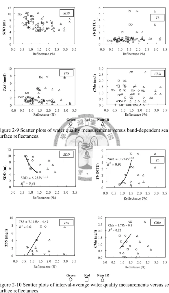
Figure 2-9 Scatter plots of water quality measurements versus band-dependent sea surface reflectances...31

Figure 2-10 Scatter plots of interval-average water quality measurements versus sea surface reflectances...31

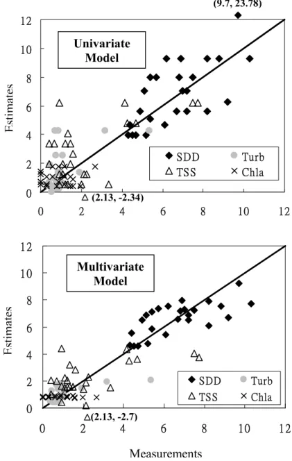
Figure 2-12 Water quality measurements versus estimates. ...33

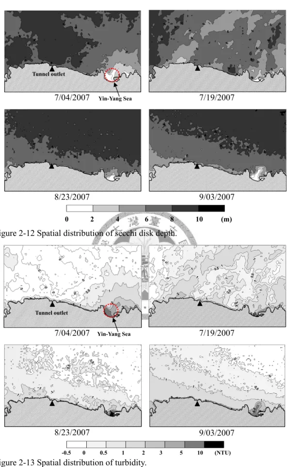
Figure 2-12 Spatial distribution of secchi disk depth. ...36

Figure 2-13 Spatial distribution of turbidity. ...36

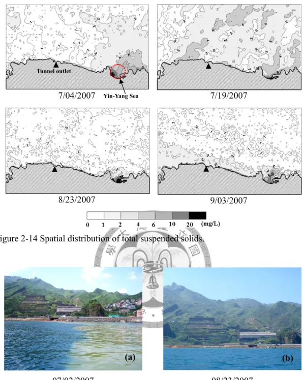
Figure 2-14 Spatial distribution of total suspended solids...37

Figure 2-15 Photos of the Yin-Yang Sea area taken during water sampling campaigns. ...37

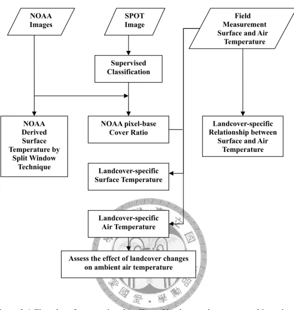
Figure 3-1 Flowchart for assessing the effect of landcover changes on ambient air temperature. ...45

Figure 3-2 Location map and pseudo-color SPOT image of the study area...50

Figure 3-3 Orthorefectified aerial photos of the study area and the field sampling route. ...50

Figure 3-4 (a) and (b): spatial variation of apparent surface temperatures derived from NOAA AVHRR images. Brighter pixels have higher apparent temperatures. (c) Area A with paddy and other vegetation. (d) Area B with residential and factory buildings...55

Figure 3-5 Results of landcover classification using multispectral SPOT images. ...59 Figure 3-6 Comparison of pixel-average surface temperatures derived by the

split window technique (TSWT) and estimated using landcover-specific

surface temperatures (T ). ...59

Figure 3-7 Vertical temperature profiles of different landcover types...63

Figure 3-8 Landcover-specific empirical relationship between the air temperature at 2m height (Ta) and surface temperature (Ts). ...63

Figure 3-9 Schematic illustration of procedures of calculation of pixel-average air temperature over a NOAA pixel. ...64

Figure 3-10 Empirical relationships between within-pixel coverage ratios of different landcover types and pixel-average air temperature. ...69

Figure 3-11 Illustrative example of the prevalent, blind and forced conversion. ...71

Figure 4-1 Northern Taiwan and the upstream basin of the Shihmen reservoir. ...81

Figure 4-2 False-color representations of SPOT images from 1999 to 2004. ...83

Figure 4-3 The proposed cloud screening procedure...87

Figure 4-4 A schematic three-by-three window for texture calculation. ...88

Figure 4-5 Example of cloud screening using the image acquired on 2004/02/10...88

Figure 4-6 Schematic plot of VI-Ts space. ...92

Figure 4-7 The SPI series for GaoYi station with a 10-day period time scale from 1999 to 2004 ...93

Figure 4-8 Classified SPOT image of the study area from 1999 to 2004...96

Figure 4-9 NDVI histograms of the six years...97

Figure 4-10 Trends of mean NDVI and cumulative SPI values. ...97

Figure 4-11 Mean NDVI and cumulative SPI values ...98

Figure 4-12 Comparison of SPOT and AVHRR images (a) SPOT false-color image, (b) classified SPOT image, (c) NDVI map derived from AHVRR, (d) NDVI map derived from SPOT, (e) filtered NDVI map derived from SPOT. ...101

Figure 4-13 The regression result of NDVI values derived from AHVRR images and filtered SPOT images...102

Figure 4-14 Relationships between the NDVI value and the coverage ratios of vegetation and built-up areas. ...102

Figure 4-15 Comparison of drought year and non-drought year for 12 months...105

Figure 4-16 Vegetation dynamics of 2002 in VI-Ts space...107

Figure 4-17 Vegetation dynamics of 2004 in VI-Ts space...107

Figure 4-18 An upgraded version of the schematic plot of VI-Ts space...109

Chapter 1 Introduction

1.1 Environmental monitoring and remote sensing techniques

Rapid development of remote sensing techniques helps scientists monitor environment resources in an efficient way. In natural resources, water resource and global warming are two major issues that are highly concerned. In the dissertation, three kinds of environment resources monitoring and assessment – water quality estimation, the effect of landcover change on air temperature, and drought effect on forest – are specifically discussed.

Water resource studies can be divided into two groups which mainly concern water quantity and quality. The former group measures and monitors the spatial distribution and the movement of water as it progresses through the hydrologic cycle; the latter group adopts remotely sensed data to estimate water quality and yields a distribution map of water quality. The later kind of application is usually difficult to obtain regional spatial information using in situ observations because the poor availability of in situ data limits the ability to assess the regional water quality. However, the

advantages of remotely sensed satellite data, a repetitive coverage and synoptic view over the area of interest, are able to resolve this problem.

Besides water issues, air temperature is another important environmental factor directly affecting human life. In recent years, global warming and urbanization are considered as major cause of air temperature rising. Urbanization, in general, converts water bodies and vegetated surface into paved road or built-up area, coming in the wake of ambient air temperature rising. Cheng et al. (2008) and Yokohari et al. (2001) reported that change of land-cover/ land-use from paddy fields into buildup results in rise of ambient air temperature about 2-3°C. Land surface temperature can be

remotely sensed by detecting the thermal infrared electromagnetic radiation in the 3 – 14 μm portion of the spectrum. The AVHRR (Advanced Very High Resolution Radiometer) operated by the NOAA (National Oceanic and Atmospheric Administration) is capable of calculating surface temperature by channel 4 and channel 5. Air temperature can further be calculated by an empirical relationship between land and air temperature. Concerning the details of how to assess the effect of landcover change on air temperature by multi-resolution remote sensing images, please refer to chapter three.

Drought is an insidious natural hazard that originates from a long-lasting deficiency of precipitation (Wilhite, 2005; Wilhite and Glants, 1985). During drought progress, in the view of agriculture, insufficient water supply to vegetation results in reduction of yield. In the end part of drought progress, water shortage depletes the supply for domestic and industrial purposes and consequently results in vast cost of society and economy.

Insufficient water supply to vegetation will reduce the rate of photosynthesis process and keep stomata close from water loss. Consequently, air exchange between ambiance and plant reduces and it will lead to higher canopy temperature. If air temperature remains high without sufficient water supply, chlorophyll contents will decrease. Drought could change surface bio-physical factors such as, land surface temperature and surface reflectance feature. Combination of these factors may provide useful information for quantitative monitoring of spatial and temporal distribution of drought (Ghulam et al., 2007).

From the temporal viewpoint, drought development is a creeping process which makes detecting the onset time a tough task. From a spatial perspective, the influence

of drought is cumulative and wide-extended without a clear boundary. In the light of the advantages of synoptic spatial coverage and routine availability of satellite images, satellite remote sensing technique is the most appropriate tool to monitor drought effect on forest.

1.2 Objectives

The first objective is to estimate water quality by remote sensing data and assess the performance of the estimation models. An integration of remote sensing techniques and water sampling is worth pursuing, since water sampling in vast water bodies is time and labor consuming. We reviewed water quality estimation models using remote sensing images for inland, estuary and coastal water bodies. Most of the estimation models are applied for estimating single water quality variable. However, natural water bodies are mixture of water and other constituents including suspended solids, dissolved organic matters, zooplankton, etc. These constituents affect the reflectance in different wavelength of spectrum. Such wavelength-dependent combined effects should be reflected in water quality estimation model. Therefore, we proposed the multivariate model for water quality estimation by atmospheric-corrected multispectral reflectances. A scheme of retrieval of water surface reflectance with remote sensing images, can be used in a local scale area, is proposed. The concept of a multivariate model for water quality estimation can be applied to inland waters (pounds, lakes, reservoirs), estuary and coastal waters.

The second objective of this study is to quantitatively evaluate the effect of landcover types on ambient air temperature by remote sensing images and to understand the inter-relationships of different landcover types in a region. We showed the theoretical details of the land surface temperature estimation by remotely sensed

thermal infrared energy. We established the landcover-specific empirical relationship between the air temperature at 2m height and surface temperature for the study area.

We proposed a new assessment method to evaluate the influence of landcover/

landuse changes on ambient air temperatures.

The final objective is to assess drought effect on forest. Six SPOT (Satellite Pour l'Observation de la Terre) satellite images with a spatial resolution of 20 m, taken in each May from 1999 to 2004, are used to classify drought severity. The relationship between NDVI and SPI is established and the drought classification by NDVI is proposed. In addition, series of AVHRR (Advanced Very High Resolution Radiometer) images, taken in year 2002 and 2004, are used to assess seasonal dynamic of forest in the feature space of vegetation index and surface temperature.

1.3 Structure

This dissertation is composed of five parts. Chapter 1, introduction, gives readers the rough concept of environmental monitoring and assessment by remote sensing techniques. In this chapter, we clarify the selected issues of environmental monitoring discussed in the dissertation. Chapter 2 elaborates on the application of remote sensing images to water quality estimation. Chapter 3 describes how to assess the influence on ambient air temperature due to landcover change. Chapter 4 shows the application of multi-sensor to drought classification and assessment. The final part is summary and suggestions.

References

Cheng, K. S., Su, Y.F., Kuo, F.T., Hung, W.C., Chiang, J.L. (2008). Assessing the effect of landcover changes on air temperature using remote sensing images - A pilot study in northern Taiwan. Landscape and Urban Planning, 85, 85-96.

Ghulam, A., Qin, Q., and Zhan, Z. (2007). Designing of the perpendicular drought

index. Environmental Geology, 52, 1045-1052.

Wilhite, D. A., and Glantz, M.H. (1985). Understanding the drought phenomenon: The role of definitions. Water International, 10(3), 111-120.

Wilhite, D. A., Ed. (2005). Drought and water crisis: science, technology, and management issues, Florida: CRC Press.

Yokohari, M., Brown, R.D., Kato, Y., Yamamoto, S. (2001). The cooling effect of paddy fields on summertime air temperature in residential Tokyo, Japan.

Landscape and Urban Planning, 53, 17-27.

Chapter 2 Water quality monitoring using remotely sensed data

2.1 Introduction

Conventional water quality monitoring depends on taking water sample in situ and analyzing it in laboratory. This procedure is not only time and labor consuming but to get distributed point data in a study area. Remotely-sensed data acquired from satellite can provide a cost-effective procedure for mapping water quality. The advantages of satellite data over conventional sampling procedures include repetitive coverage of an interesting area in a short period, and a synoptic view which provides almost instantaneous spatial data over the area of interest and is unobtainable by conventional procedure.

The sensor on satellite measures the radiative signal from a water surface to the sensor. Water quality can be estimated by the radiative signal. The studies of applying remote-sensed data to water quality monitoring have been proposed before 30 years ago. Coastal Zone Color Scanner (CZCS) is the first satellite launched by United States of America in 1978 specifically designed to sense ocean color. In the past three decades, many countries launched their own satellites for ocean color monitoring including SeaWiFS, MODIS etc. However, most of the ocean color observation satellites have spatial resolution of 1 km. The image data of this spatial scale limits the capability of monitoring inland water or near shore coastal water monitoring.

Under this situation, a satellite with meter-scale spatial resolution, such as SPOT or Landsat, is more adapted for the application.

In general, water quality study can be divided into two categories, inland waters and ocean waters. Reservoirs and lakes are kind of inland waters which are easily affected by land-source substance. Suspended solid material carried in by upstream

inflow trapped in impounded water bodies may have long-lasting effect on impounded water quality. The constituents of inland waters are more complex than ocean waters. Besides suspended solid material, nutrients such as phosphate and nitrogen are other major constituents in impounded water bodies. Inland water quality will be affected by settling of sand particles and eutrophication. Therefore, in inland waters, the data ranges of water quality variables, such as total suspended solids, turbidity and chlorophyll-a concentration, are larger than those in ocean waters. There are many successful applications for inland water quality monitoring (Cheng and Lei, 2001; Giardino et al., 2001; Huang, 2006; Kloiber et al., 2002; Lin, 2005; Östlund et al., 2001; Tan, 2006; Verdin, 1985; Wang et al., 2004; Wu, 2001).

Morel and Prieur (1977) suggested that ocean waters can be divided into two cases according to constituents of ocean waters. The optical property of Case I ocean water is mainly affected by phytoplankton, also named as original open ocean water body.

Non-algal particle (NAP) is the dominating factor in Case II ocean water. Near shore water and coastal water quality are constantly affected by upstream flow discharge which may contain high concentration sediments, especially during high-flow periods.

Flushed by seawater, suspended solid material in coastal water may be mixed. Thus the characteristics of creeping impact and low immediate effect make it difficult to sense the emerging consequences which may be severely deleterious and irreversible on coastal ecosystem. For example, Tomascik and Sander (1985) and Hoegh-Guldberg et al. (2004) reported that change to coastal discharge is one of the most serious threats to coral reef ecosystem. Thus, understanding the long term effect of sediments carried in the upstream discharge on coastal water quality necessitates a routine monitoring scheme.

The optical properties of Case II water shows that when concentration of NAP is

higher the reflectances of visible band and near infrared band will arise; meanwhile, the influence of chlorophyll-a concentration on reflectance will decrease (Doxaran et al., 2002; Lodhi et al., 1997; Oyama et al., 2007). Runquist et al. (1996) measured the

reflectances of water surface with different chlorophyll-a concentration (156~277μg/L, 340~2190μg/L). The spectral pattern shows that when chlorophyll-a concentration increases, the reflectances of green and near infrared bands increase with it;

meanwhile, the reflectance of blue and red bands decrease (Figure 2-1). The spectral pattern is more regular under high chlorophyll-a concentration (340~2190μg/L). The minor irregularities in the spectral pattern of lower chlorophyll-a concentration water surface probably occur because overall chlorophyll levels are very low (156~277μg/L). In general, chlorophyll-a concentration in Case II water is extreme low (0~3μg/L). The spectral pattern in Case II water may be more insignificant. It causes difficulties for monitor water quality by satellite data. Therefore, an appropriate monitoring model is necessary for a synoptic water quality monitoring.

Over the past three decades, the univariate models using only one water quality variable as dependent variable are proposed in many applications (summarized in Table 2-1). However, the water body is a mixture of seawater, suspended solids, color dissolved organic matters, and phytoplankton etc. The sea surface reflectance of a specific wavelength is interworked by those constituents. Some authors mentioned that the complexity of constituents in nature water interferes the spectral identification of water quality and affects the accuracy of estimation model. However, there is no solution suggested in the literature (Giardino et al., 2001;Wang et al., 2004).

Considering the wavelength-dependent combined effect must be reflected in the water quality estimation model, a multivariate model is proposed in this study. The

Figure 2-1 Reflectance factor of water surface with varied Chlorophyll-a concentration (Runquist, 1996).

Green Red

NIR

Green Red

NIR

Table 2-1 Univariate models.

Impounded waters

Study Area Sensor Variable Type Reference

Flaming Gorge Reservoir MS SSD, Chla Exp, Poly Verdin, 1985

Moon Lake MS TSS Poly Ritchie and Cooper, 1988

Iseo Lake, Italy TM SDD, Chla Poly Giardino et al., 2001 Yung-He-Shan Reservoir SPOT SDD, Chla, Tb, TP Power, Poly Wu, 2001

Erken Lake, Sweden TM, CASI TSS, Chla Power, Poly Östlund et al., 2001 Four lakes in Finland AISA*, MERIS SDD, Tb, Chla Poly Koponen et al., 2002

Lakes in Twin City TM, MS SDD Exp Kloiber et al., 2002

Frisian Lakes TM, SPOT TSS Exp Dekker et al., 2002

Shenzhen Reservoirs TM TOC, BOD, COD Poly Wang et al., 2004 Tseng-Wen Reservoirs FS II TSS, Turb, Chla Poly Huang, 2006

Coastal water or Estuary water

Study Area Sensor Variable Type Reference

San Francisco Bay MS TSS, Tb Poly Khorram, 1981

San Francisco Bay Daedalus* Chla Poly Catts et al., 1985

Neuse River Estuary MS SAL, Chla, Tb, TSS Poly Khorram and Cheshire, 1985

Adriatic Sea TM, CZCS TSS, Chla Power Tassan, 1987

Swasea Bay NERC* TSS, SAL Exp Rimmer et al., 1987

North Sea AVHRR TSS Power Prangsma and Roozekrans, 1989

New Jersey’ coast TM Chla Poly Bagheri and Dios, 1990

Augusta Bay TM SDD, Tb, Chla, Temp Power Khorram et al., 1991 Western Australia Coast TM SDD, Chla, Pha Exp, Poly Lavery et al., 1993 Western Australia Coast TM SDD, Chla Exp Pattiaratchi et al., 1994 Indonesian seas TM, SPOT TSS, PIG Exp Populus et al., 1995 Lakes and Coastal water

in Finland

TM, MODIS, MERIS

SDD, TSS, Chla, Turb Poly Härmä, et al. 2001

Gironde Estuary SPOT TSS Exp Doxaran et al., 2002

New York Harbor TM, MODIS SDD, Chla Power Hellweger et al., 2004 Florida near-shore area SeaWiFS Chla Power, Poly Cannizzaro and Carder, 2006

*: Airborne Sensor; MS: Landsat Multispectral Scanner; TM: Landsat Thematic Mapper; FS II: Formosat II Exp: Exponential ; Poly: Polynomial;

TSS: Total Suspended Solid; Tb: Turbidity; SDD: Secchi Disk Depth; Chla: Chlorophyll-a concentration

Pha: Phaeophytin; TOC: Total Organic Carbon; BOD: Biochemical Oxygen Demand; COD: Chemical Oxygen Demand;

Temp: Temperature; TP: Total Phosphorus; SAL: Salinity;

atmospheric corrected water surface reflectances of SPOT images are the independent variables in proposed model. The water quality variables selected in this study are secchi disk depth (SDD), turbidity (Tb), total suspended solids (TSS) and chlorophyll-a concentration (Chla). SDD is a measure of water transparency in seawaters and is related to water turbidity and the radiance onto water surface.

Turbidity and total suspended solids are the indicators to show organic and inorganic particle amount in a water body. The chlorophyll-a concentration is well-correlated to the amount of phytoplankton. These four variables are commonly used to assess the water quality in Case II waters.

2.2 Study area and materials

Yuan-Shan-Tzu (YST) Diversion Tunnel is designed to divert flood flow from the upper Keelung River Basin to a discharge outlet at the northern tip of Taiwan. The YST tunnel, completed in 2003 with a diameter of 12 m and 2.48 km in total length, is capable of diverting approximately 81% (1,310 m³/s) of the 200-year flood flow (1,620 m³/s) at a cross section near the inlet of YST tunnel. The coastal area near the outlet of the Yuan-Shan-Tzu Diversion Tunnel in northern Taiwan is the typical Case II water and is selected as study area in this article (Figure 2-2). A radiometric control area (RCA) of approximately 30m×60m is selected in Figure 2-2 for spectral reflectance calibration. The RCA is a horizontal paved open area with homogeneous and stationary surface reflectance and no adjacent obstruction (see Figure 2-3).

During July to November of 2007, a few water sampling campaigns were conducted in a coastal area of tunnel outlet. The sampling dates and relevant storm information are shown in Table 2-2. Water samples were taken within 0 – 20 cm range below the sea surface at eight locations (see Figure 2-2) during each sampling

campaign. Global positioning systems were used to guide the sampling vessel to the desired sampling locations. Considering the west-to-east surface current direction of the season, the sampling area extends from a little northwest of the outlet to about 2 km to the east of the outlet. Sampling point 4 is located within an area known as the Yin-Yang Sea. Geology of the near Yin-Yang Sea area has a large amount of pyrite that does no dissolve easily in water. The Yin-Yang Sea area, just offshore from an old metal mining township, frequently receives runoff containing high iron ion concentration, making the sea surface visually distinct. Secchi disk depth and turbidity were measured in situ and water samples were taken to the Environmental Chemistry Lab at the National Taiwan University for analyses of total suspended solids and chlorophyll-a concentration.

The water quality analysis methods used in this study are proposed by the Environmental Analysis Laboratory, EPA, Executive Yuan, R.O.C. Secchi disk depth records the depth that naked eye cannot see the secchi disk in water. Turbidity is measured by a portable turbidity meter (2100P, HACH, USA) with unit of Nephelometric Turbidity Unit (NTU). Secchi disk depth and turbidity are measured in situ during each sampling campaign. Total suspended solids is determined by pouring

a carefully measured volume of water through a pre-weighted glass-fiber filter (GF/F, 47mm diameter, 0.7μm pore size), then weighting the filter again after drying to remove all water. The gain in weight divided the volume of sample water is the measure of total suspended solids with unit of mg/l. Chlorophyll-a can be extract by ethanol from a pre-weighted glass-fiber filter which volume of water already poured through, then measure the absorptions at 665 and 750nm. Chlorophyll-a concentration can be calculated by the absorptions at 665 and 750nm. The methods used for water quality variables are listed in Table 2-2.

A few multispectral images from SPOT satellites with acquisition dates close to the dates of sampling campaign were also collected (see Table 2-3). During and immediately after the Wipha and Krosa typhoon events, the study area were almost completely under cloud cover, and thus no SPOT images were collected. The multispectral SPOT images include images of three spectral bands – green (0.5–0.59 μm), red (0.61–0.68 μm), and near infrared (0.78–0.89 μm), with pixel resolution of 20 m for SPOT-4 or 10 m for SPOT-5.

Table 2-4 summarizes statistical properties of the three water quality variables. Two sampling campaigns (09/20/2007 and 10/08/2007) took place one day after activation of flood diversion. Comparison of the water quality data of the no-diversion and post-diversion periods is shown in Figure 2-4. Differences in medians and ranges of TSS, Tb and SDD are apparent. For example, median of SDD drops from 6.8 m of the

no-diversion period to 3.8 m of the post-diversion period, whereas median of TSS increases from 1.6 mg/L of the no-diversion period to 5.2 mg/L of the post-diversion period. Also, excluding the outliers, the ranges of the water quality variables of the no-diversion and post-diversion periods are almost non-overlapping.

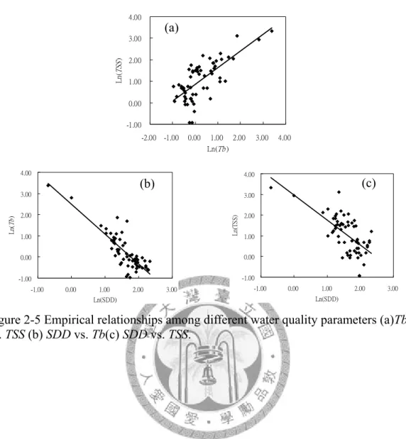
Before pursuing establishment of water quality estimation models using the water quality data and remote sensing images, we conducted a careful check on measurements of water quality variables. The purpose of such data check is to screen out data which might have been contaminated by inappropriate sampling of water samples or erroneous measurement in the lab. In general, the Secchi disk depth, total suspended solids, and turbidity are inter-related, as showed in following equations and demonstrated in Figure 2-5. The points marked by dashed-circles are significantly inconsistent with such correlation, and thus are excluded in subsequent analyses.

Similar relationships between the Secchi disk depth and the turbidity are showed in few researches (Gao et al., 2008; Gryson et al., 1996; Koponen et al., 2002; Lewis, 1996; Pavanelli and Bigi, 2005).

(

^SDD

)

^{1.71 0.5ln}

( )

^Tb

ln = − (R² =0.71) (2-1a)

( )

^{TSS 0.86 0.77ln}

( )

^Tb

ln = + (R² =0.52) (2-1b)

( )

^{TSS 2.97 1.21ln}

(

^SDD

)

ln = − (R² =0.45) (2-1c)

2.3 Retrieval of reflectance

Mobley (1994) described the optical properties of natural water are conveniently divided into two mutually exclusive classes: inherent and apparent. Inherent optical properties (IOP’s) are those properties that are independent of the ambient light field.

The two fundamental IOP’s are the absorption coefficient and the volume scattering function which can quantitatively describe the solar radiance transfer process.

Apparent optical properties (AOP’s) are those properties that depend both on the medium and on the geometric structure of the ambient light field, and that display enough regular features and stability to be useful descriptors of the water body. The spectral remote-sensing reflectance is one of the most important AOP. The spectral remote-sensing reflectance, hereafter which is short as reflectance, is used to construct the experience model in this study.

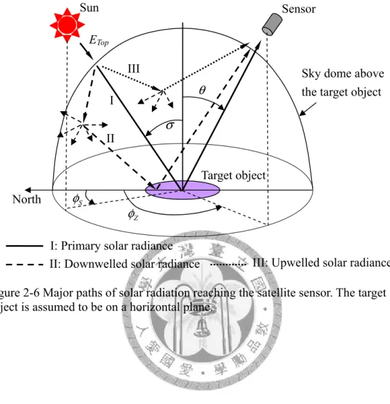
In satellite remote sensing application, the major paths of solar radiation reaching the sensor are depicted in Figure 2-6. The primary solar radiance (path I) accounts for the solar irradiance onto the target object, and then reflected back to the atmosphere, and finally arrives at the sensor. The downwelled solar radiance (path II) is the atmospheric scattered solar radiance incident on and reflected away from the target object before reaching the sensor. The upwelled solar radiance (path III) is the radiance scattered by the atmosphere and directly reaching the sensor without getting

Figure 2-2 Study area in northern Taiwan (The numbers represent the sample sites).

Figure 2-3 The radiometric control area (RCA).

Taiwan

Study Area

2 3

4 5 8 7

Yin-Yang Sea 1 6

Tunnel Outlet RCA

Approximate sampling locations

0 4 8 12

SDD (m)

Normal Diversion

0 1 2 3 4 5 6

Tb (NTU)

Normal Diversion

Secchi disk depth Turbidity

0 2 4 6 8 10

TSS (mg/L)

Normal Diversion

0 1 2 3

Chla (ug/L)

Normal Diversion

Total suspended solids Chlorophyll-a concentration Figure 2-4 Box plots of water quality data of no-diversion and post-diversion periods.

No-diversion Post-diversion No-diversion Post-diversion

No-diversion Post-diversion No-diversion Post-diversion

SDD (m) Tb (NTU)

TSS (mg/L) Chla (μg/L)

-1.00 0.00 1.00 2.00 3.00 4.00

-2.00 -1.00 0.00 1.00 2.00 3.00 4.00 Ln(Tb)

Ln(TSS)

-1.00 0.00 1.00 2.00 3.00 4.00

-1.00 0.00 1.00 2.00 3.00

Ln(SDD)

Ln(Tb)

-1.00 0.00 1.00 2.00 3.00 4.00

-1.00 0.00 1.00 2.00 3.00

Ln(SDD)

Ln(TSS)

Figure 2-5 Empirical relationships among different water quality parameters (a)Tb vs. TSS (b) SDD vs. Tb(c) SDD vs. TSS.

(c) (a)

(b)

Table 2-2 Methods of water quality analysis.

Water quality variable Methods Unit

Chlorophyll-a conc. NIEA E508.00B μg/L

Turbidity NIEA W219.52C NTU

Secchi disk depth NIEA W221.50A m

Total suspended solid NIEA W210.57A 103⁰C-105⁰C mg/L Table 2-3 Dates of water sampling and SPOT image acquisition.

Sampling date

SPOT image acquisition date

Relevant storm events

Volume of diverted flow (m³) 7/02/2007 7/04/2007

(SPOT-4) No storm 0

7/18/2007 7/19/2007

(SPOT-4) No storm 0

8/15/2007 NA^a No storm 0

8/23/2007 8/23/2007 (SPOT-5)

Typhoon Sepat

(8/16~8/19) 0

9/07/2007 9/03/2007

(SPOT-5) No storm 0

9/20/2007 NA^a

Typhoon Wipha^b (9/17~9/19)

1,051,200

10/08/2007 NA^a Typhoon Krosa^b

(10/4~10/7) 16,133,400

11/14/2007 NA^a No storm 0

aSatellite images were not collected due to high percentage of cloud cover.

bFlow diversion activated.

Table 2-4 Statistical properties of water quality variables.

Mean Standard

deviation Maximum Minimum

Secchi disk depth (m) 5.40 2.13 10.30 0.50

Turbidity (NTU) 2.20 4.22 29.50 0.38

Total suspended solid (mg/L) 4.36 4.97 28.00 0.40

Chlorophyll-a conc. (μg/L) 0.79 0.69 2.67 0.00

Total number of samples: 61

in contact with the target object.

Mobley (1994) defined the spectral remote-sensing reflectance, in this study is called reflectance, as the water-leaving radiance divided by irradiance onto water surface. Spectral remote-sensing reflectance, which is abbreviated as reflectance in this study, is presented as:

( ) ( )

( )

φλ σ λ φ

λ θ σ φ φ

θ E

R_{rs S Z} L , ^S, ^Z, , ,

, ,

, = (2-2)

where

R = the water-leaving radiance rs

L = the water-leaving radiance

θ = view angle in sensor-target direction φ = sensor azimuth angle Z

φS =sun azimuth angle σ = the sun angle

E = the solar irradiance reaching water surface λ = wavelength in μm.

The amount of solar radiance reaching the satellite sensor can be expressed as:

(

θ^,φZ^,λ

) (

θ^,φS^,φZ^,σ^,λ

) ( )

τ2 λ u

(

θ^,φZ^,λ

)

S L L

L = ⋅ + (2-3)

where τ₂ is the atmospheric transmittance along the target-sensor path and L is _u upwelled solar radiance ( also known as path radiance). The water-leaving radiance can further expressed as:

(

θ^,φS^,φZ^,σ^,λ

)

⁼

L

( ) ( )

πφ σ λ φ

σ θ λ

τ1 ^cos rs ^, S^, Z^{, ,} Top

E ⋅ ⋅ ⋅R +

( ) ( )

πλ λ ^rs

D

E R

F⋅ ⋅

(2-4)

where

ETop= the exoatmospheric solar irradiance

τ1 = the atmospheric transmittance along the sun-target path ED = the downwelled irradiance from the sky dome onto the target

F = the obstruction factor.

The obstruction factor in equation (2-4) accounts for the proportion of irradiance that may be obstructed by adjacent objects or surface slope of the target. If the target object is on a horizontal surface and free of adjacent object obstruction, the factor F equals 1. It is also worthy to note that the sun and view angles are defined with reference to the normal of the target surface. If the target is located on a slope, the sun and view angles will need to be adjusted accordingly. Readers are referred to Schott (1997) for detailed calculation of solar radiances arriving at the sensor.

The reflectance Rrs

(

^θ,φS^,φZ^,σ,λ

)

varies with spectral wavelength and orientation angles. If the target object is assumed to be a diffuse reflector with a constant reflectance Rrs

( )

^λ in all directions, we then have

(

^θ,φZ^,λ

)

⁼

LS

(

^{ETop ⋅τ1}

( )

^{λ ⋅cosσ +F⋅ED}

( )

^λ

)

^{⋅ Rrs}_π

^{( ) ( )}

^{λ ⋅λ2 λ}

(

θ^,φZ^,λ

)

Lu

+

(2-5)

On the right hand side of the above equation, only the reflectance Rrs

( )

λ represents the physical property of the target surface. The upwelled radiance L_u does not even get into contact with the target.

Environmental monitoring using remote sensing images often requires derivation of physical properties (reflectance, for example) of the target objects from satellite images. Unfortunately, the upwelled radianceL_u, the atmospheric transmittance τ₁ andτ₂, the downwelled irradianceE_D, and the exoatmospheric solar irradiance ETop

are generally not available for most applications, and we have to resort to other means for estimation of the reflectance.

For most local-scale environmental monitoring applications,L_u,τ₁^,τ2^,ED, and

Figure 2-6 Major paths of solar radiation reaching the satellite sensor. The target object is assumed to be on a horizontal plane.

Sun Sensor

Sky dome above the target object

Target object North φ_S

φZ

θ σ

I: Primary solar radiance III I II

II: Downwelled solar radiance III: Upwelled solar radiance ETop

ETop can be assumed constant (or spatially invariant) within the study area. While on the contrary, the sun angle σ and the obstruction factor F are dependent on the surface slope of the target, and the reflectance ^Rrs

( )

^λ is dependent on surface cover of the earth. Their values may vary from pixel to pixel within a scene. If only pixels on horizontal surface and free of adjacent obstruction are considered (F = 1), Equation (2-5) may be expressed as:

(

^θ,φZ^,λ

)

⁼

LS

( ( ) ( ) ) ( ) ( )

λ λ

π λ λ σ

λ

τ1 ⋅cos + ⋅ ⋅ 2

⋅ D ^rs

Top

E R E

(

θ^,φZ^,λ

)

Lu

+

=k1⋅R_rs

( )

λ +k2

(2-6)

where

( ) ( )

(

^{τ1 λ σ λ}

)

^τ2_π

^{( )}

^λ

1 = ETop ⋅ ⋅cos +ED ⋅

k

(

θ^,φ ^,λ

)

2 Lu Z

k =

A common practice dealing with the upwelled radiance Lu

(

θ^,φZ^,λ

)

in satellite remote sensing is the dark object subtraction (DOS) method (Chavez, 1988; Cheng and Lei, 2001; Teng et al., 2008). The basic concept of the DOS method is to identify very dark features within the scene. The minimum scene radiance is set to be the upwelled radiance based on the assumption that it represents the radiance from a pixel with near zero reflectance. If the minimum scene radiance is subtracted from the radiance of each individual pixel, the processed image is then assumed free of atmospheric scattering effect.

After removing the upwelled radiance Lu

(

θ^,φZ^,λ

)

using the DOS method, the DOS-adjusted radiance ^L'S

(

^θ,φZ,λ

)

is linearly related to the surface reflectance, i.e.:

(

^{θ,φ ,λ}

)

⁼

' Z

LS LS

(

^θ,φZ^,λ

)

⁻ Lu

(

θ^,φZ^,λ

)

=k1⋅Rrs

( )

λ (2-7) Based on the linear relationship between L^'_S andRrs

( )

λ , we derive a surface

reflectance estimation scheme through reflectance calibration in a radiometric control area (RCA).

In this study a radiometric control area of approximately 30 m × 60 m was chosen for spectral reflectance calibration. The RCA is a horizontal paved open area with homogeneous and stationary surface reflectance and no adjacent obstruction (see Figure 2-3). It is located in a restricted and free of public access harbor area. The wavelength-depended surface reflectance of RCA is then calibrated using a variable spectral radiometer (VSR) which is equipped with two spectral-variable filters capable of detecting spectral radiances in various 7 nm-wide windows within the 0.40 – 0.72 μm and 0.65 – 1.1 μm ranges respectively (Figure 2-7). The VSR was moved around within the radiometric control area taking multispectral images. When taking images within the RCA, a standard reflectance disk which has been pre-calibrated to have Rrs^Disk

( )

λ ^≈1 over the 0.25 – 1.1 μm wavelength range was also placed within the viewing area. Reflectance of the radiometric control area is then calculated as the ratio of average radiance from RCA to average radiance from the standard reflectance disk, i.e.:

( )

^λ Disk ^rsDisk

( )

^λ

S RCA RCA S

rs R

L

R = L ⋅ (2-8)

where Rrs^RCA

( )

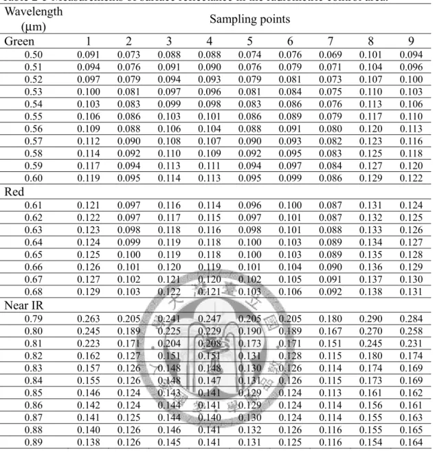
^λ is the reflectance of RCA, andL^RCAS andL^DiskS are respectively average radiances received at VSR sensor from the RCA surface and from the standard reflectance disk. For RCA reflectance calibration, the effect of upwelled radiance can be neglected since the VSR is placed near the ground surface. Table 2-5 lists measurements of surface reflectance in the radiometric control area and area average reflectance with respect to various spectral wavelengths are also shown in

Figure 2-8. The RCA-average reflectance corresponding to green, red and near infrared SPOT spectral bands (hereafter referred to as the RCA band reflectances) are calculated to be 0.097, 0.113, and 0.161%, respectively. The RCA band reflectances are considered constant since the land surface condition within the RCA is relatively homogeneous and stationary.

Assuming the sea surface is horizontal, the DOS-adjusted radiances of a pixel A in the RCA and a pixel B on the sea surface are respectively expressed by:

(

θ φZ λ

)

rs^A

( )

λ

A

S k R

L' , , = 1⋅ (2-9)

(

θ φZ λ

)

rs^B

( )

λ

B

S k R

L' , , = 1⋅ (2-10)

where R and _rs^A R are the reflectance of RCA pixel A and sea surface pixel B, _rs^B respectively. Combining Equation (2-9) and Equation (2-10) and rewriting the reflectance of sea surface pixel B as:

( ) ( )

( ) (

θ φ λ

)

λ φ θ

λ λ ^{, ,}

, ,

'

' Z

B S Z

A S

A B rs

rs L

L

R R ⎥⋅

⎦

⎢ ⎤

⎣

=⎡ (2-11)

Practically, ^'

(

θ^,φZ^,λ

)

A

LS and Rrs^A

( )

λ are respectively replaced by the average radiance and reflectance of RCA, and

( ) ( )

( ) (

θ φ λ

)

λ φ θ

λ λ ^{, ,}

, ,

'

' Z

B S Z

RCA S

RCA B rs

rs L

L

R R ⋅

⎥⎥

⎦

⎤

⎢⎢

⎣

=⎡ (2-12)

where ^'

(

θ^,φZ^,λ

)

RCA

LS represents the average value of DOS-adjusted radiances within RCA and Rrs^RCA

( )

^λ is the RCA band reflectance. The reflectance calibration ratio

( ) (

^{θ φ λ}

)

λ ,

' ,

Z RCA S

RCA rs

L

R in above equation may vary with SPOT scenes since ^'

(

θ^,φZ^,λ

)

RCA

LS

varies due to scene variations in orientation angles and atmospheric transmittance.

Table 2-6 summarizes reflectance calibration ratios of individual SPOT multispectral images.

2.4 Water quality estimation model assessment

In order to map the spatial distribution of water quality variables using remote sensing images, it is necessary to establish water quality estimation models based on reflectance of sea surface. A few simple or multiple regression models have been proposed in the literature (Bagheri and Dios, 1990; Cannizzaro and Carder, 2006;

Catts et al., 1985; Giardino et al., 2001; Härmä et al., 2001; Hellweger et al., 2004;

Huang, 2006; Khorram, 1981; Khorram and Cheshire, 1985; Khorram et al., 1991;

Kloiber et al., 2002; Lavery et al., 1993; Oyama et al., 2007; Pattaratchi et al., 1994;

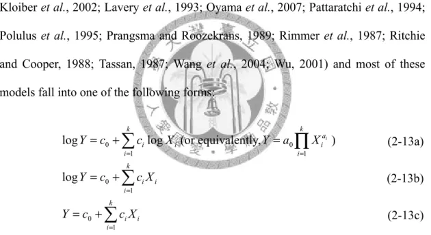
Polulus et al., 1995; Prangsma and Roozekrans, 1989; Rimmer et al., 1987; Ritchie and Cooper, 1988; Tassan, 1987; Wang et al., 2004; Wu, 2001) and most of these models fall into one of the following forms:

∑=

+

= ^k

i ci Xi

c Y

1

0 log

log (or equivalently, ∏

=

= ^k

i a iⁱ

X a Y

1

0 ) (2-13a)

∑=

+

= ^k

i ciXi

c Y

1

log 0 (2-13b)

∑=

+

= ^k

i ciXi

c Y

1

0 (2-13c)

where Y represents a water quality variable and Xi can be reflectance of a specific spectral band, ratio of reflectances of different spectral bands, or other arithmetic calculation of band reflectances.

In order to choose appropriate models for water quality mapping, we first examined scatter plots of water quality measurements versus band-dependent sea surface reflectances, as shown in Figures 2-9(a)-(d). Although the data points are widely dispersed, particularly in lower measurement ranges, measurements of turbidity and

Table 2-5 Measurements of surface reflectance in the radiometric control area.

Wavelength

(μm) Sampling points

Green 1 2 3 4 5 6 7 8 9

0.50 0.091 0.073 0.088 0.088 0.074 0.076 0.069 0.101 0.094 0.51 0.094 0.076 0.091 0.090 0.076 0.079 0.071 0.104 0.096 0.52 0.097 0.079 0.094 0.093 0.079 0.081 0.073 0.107 0.100 0.53 0.100 0.081 0.097 0.096 0.081 0.084 0.075 0.110 0.103 0.54 0.103 0.083 0.099 0.098 0.083 0.086 0.076 0.113 0.106 0.55 0.106 0.086 0.103 0.101 0.086 0.089 0.079 0.117 0.110 0.56 0.109 0.088 0.106 0.104 0.088 0.091 0.080 0.120 0.113 0.57 0.112 0.090 0.108 0.107 0.090 0.093 0.082 0.123 0.116 0.58 0.114 0.092 0.110 0.109 0.092 0.095 0.083 0.125 0.118 0.59 0.117 0.094 0.113 0.111 0.094 0.097 0.084 0.127 0.120 0.60 0.119 0.095 0.114 0.113 0.095 0.099 0.086 0.129 0.122

Red

0.61 0.121 0.097 0.116 0.114 0.096 0.100 0.087 0.131 0.124 0.62 0.122 0.097 0.117 0.115 0.097 0.101 0.087 0.132 0.125 0.63 0.123 0.098 0.118 0.116 0.098 0.101 0.088 0.133 0.126 0.64 0.124 0.099 0.119 0.118 0.100 0.103 0.089 0.134 0.127 0.65 0.125 0.100 0.119 0.118 0.100 0.103 0.089 0.135 0.128 0.66 0.126 0.101 0.120 0.119 0.101 0.104 0.090 0.136 0.129 0.67 0.127 0.102 0.121 0.120 0.102 0.105 0.091 0.137 0.130 0.68 0.129 0.103 0.122 0.121 0.103 0.106 0.092 0.138 0.131

Near IR

0.79 0.263 0.205 0.241 0.247 0.205 0.205 0.180 0.290 0.284 0.80 0.245 0.189 0.225 0.229 0.190 0.189 0.167 0.270 0.258 0.81 0.223 0.171 0.204 0.208 0.173 0.171 0.151 0.245 0.231 0.82 0.162 0.127 0.151 0.151 0.131 0.128 0.115 0.180 0.174 0.83 0.157 0.126 0.148 0.148 0.130 0.126 0.114 0.174 0.169 0.84 0.155 0.126 0.148 0.147 0.131 0.126 0.115 0.173 0.169 0.85 0.146 0.124 0.143 0.141 0.129 0.124 0.113 0.161 0.162 0.86 0.142 0.124 0.144 0.141 0.129 0.124 0.114 0.156 0.161 0.87 0.141 0.125 0.144 0.140 0.130 0.124 0.114 0.155 0.163 0.88 0.140 0.126 0.146 0.141 0.132 0.126 0.116 0.155 0.165 0.89 0.138 0.126 0.145 0.141 0.131 0.125 0.116 0.154 0.164

Table 2-6 Scene reflectance calibration ratios of SPOT multispectral images used in this study.

Reflectance calibration ratio

( ) (

^{θ φ λ}

)

λ ,

' ,

Z RCA S

RCA rs

L R Image acquisition date

Green Red Near infrared

7/04/2007 0.00282 0.00313 0.00420

7/19/2007 0.00232 0.00249 0.00410

8/23/2007 0.00331 0.00336 0.00532

9/03/2007 0.00345 0.00342 0.00500

Figure 2-7 Variable spectral radiometer (VSR) used for reflectance calibration.

0.00 0.05 0.10 0.15 0.20 0.25

0.5 0.6 0.7 0.8 0.9

Figure 2-8 Calibrated wavelength-dependent RCA-average reflectances and band-average reflectances.

Wavelength, μm

Reflectance, %

Green Red Near IR

Band-average reflectance Standard

reflectance disk

VSR

Lens

Spectral Variable filter

CCD Lens