以光鑷與協同冷卻實現可擴展的離子阱量子電腦

(1)

國立臺灣大學理學院物理學系碩士論文

Department of Physics College of Science

National Taiwan University Master Thesis

以光鑷與協同冷卻實現可擴展的離子阱量子電腦 Scalable Quantum Computing with an Ion Crystal

Stabilized by Tweezers and Sympathetic Cooling

沈于晴 Yu-Ching Shen

指導教授：林俊達博士 Advisor: Guin-Dar Lin, Ph.D.

中華民國 106 年 12 月 December, 2017

(2)

(3)

誌謝

經過漫長的時間，終於完成畢業論文了。首先要感謝我的指導教授林俊達老師。在老師自由且不失嚴謹的指導下，我對量子光學、量子計算與如何做研究有了更深的感覺。感謝張銘顯老師與管希聖老師的建議，使這份論文更加完善。感謝實驗室的各位夥伴：冠廷、婷姐、

鎮宇、澤霈、爾祥、可維、資莘、智圓、享莨，除了平常的討論和閒聊外，在我需要幫忙時也一定可以得到你們的幫助。感謝「屁哥讀書會」的隊友們：博亞、善長、銘峰、力弘。在各自為研究奮鬥的同時，

我很享受跟你們一起讀統物、讀量物、讀場論，當然還有天南地北瞎扯的時光。你們是我最大的精神支柱。感謝同在 502 裡打拼的安良學長、泰尹、丞翔、仁宇，以及時常來 502 串門子的老錢、重陽、蕎東、

小高、沂璇。此外，感謝國術社與校隊的彥竹、翊蕾、權元、兆平、

岱蓉、珮恂、謝慈、稚然、韋君、大大大、不缺；以及一起吃拉麵的基隆人們：聖倫、爆哥、浩宸。你們讓我的研究生活從不乏味。最後，

最重要的，感謝我的爸媽無條件支持，讓我沒後顧之憂；感謝我可愛的妹妹無時無刻不幫我加油打氣。我愛你們！

(4)

摘要

如何擴展離子阱量子電腦一直以來是一項挑戰，其困難主要來自穩定離子陣列以及克服背景雜訊造成的加熱。在實現量子邏輯閘的操控上，由於要求雷射光能準確照射在某個特定的離子量子位元而不影響鄰近位元，離子間的距離必須大於雷射光寬度，而這個間距的數量級大約為微米等級。在常用的無線電頻率（radio-frequency, RF）離子阱架構下，當離子的數目越來越多時，軸向的束縛頻率須越來越小，

以保持離子間距。故當大型離子陣列用於量子計算時，首要困難就是軸向模態的頻率趨近於零，使得該方向振動難以冷卻。因此我們提出在大型離子陣列中加入光鑷來固定離子，借此引入了新的軸向振動頻率。我們計算了當離子處於背景加熱時在協同冷卻下達到穩定態時的位置不準量。我們發現光鑷增加了軸向的穩定度。此外，光鑷阻擋了徑向模態的熱傳導。這個特性保護了在不同區域的量子邏輯閘不受彼此的影響，由此可以實行平行運算。等效來說，我們可以將兩個光鑷間的離子視為一段「局部離子阱」。我們計算了局部離子阱的冷卻效率以及探討其弛豫動力學。

關鍵字：離子阱、可擴展量子計算、光鑷、協同冷卻

(5)

Abstract

Scalability of quantum computing based on trapped ions in a linear radio- frequency trap has been a challenge due to instability of crystallization and heating. To construct a large-scale ion array with single qubit addressability, the ions’ spacing must be kept a few times larger than or at least comparable to the beam size, which is of the order of microns. This implies that the longitudinal confinement vanishes as the number of ions gets very large.

Meanwhile, the collective motional modes of very low frequencies are easily thermally populated and hard to be cooled. We thus propose a scalable scheme combining the applications of optical tweezers and sympathetic cooling. We demonstrate that for a large-scale ion chain, the application of optical tweezers raises the lowest longitudinal frequency by effectively pinning the ions in space. We calculate the steady-state profile of ions’ position fluctuations given that the system exposes to heat and is also sympathetically cooled at the same time. We find that the optical tweezers can enhance the stabi- lity of the longitudinal arrangement. Also, it blocks heat propagation of the transverse motion, suggesting that the qubit gate operation based on transverse modes can be done in parallel and thus protected by optical tweezers.

This allows us to deal with only a portion defined by two edge ions that are illuminated by tweezer beams. This segment of the ion array is confined by a “local trap” provided by two effectively pinned ions. We demonstrate the relevant cooling efficiency and discuss the relaxation dynamics.

Keywords: ion trap, scalable quantum computation, optical tweezers, sym-

(6)

pathetic cooling

(7)

List of Figures

1.1 The analogous figure of Paul trap. A particle is confined in a rotating saddle-shaped potential surface. . . 4 1.2 The schematic figure of an ion trap device. (a) The standard Paul trap

formed by four parallel wires. (b) The surface-electrode ion trap [19]. . . 4 1.3 The energy level of a trapped ion. The green, blue, and red arrows corre-

spond to the carrier, blue sideband and red sideband transitions respectively. . . 5 1.4 The concept of the Cirac-Zoller gate. . . 8 1.5 The concept of the Mølmer-Sørensen gate. Bichromatic laser beams are

applied on the ions. The intermediate states are not populated because of the off resonance. The overall transitions are|ggn⟩ ↔ |een⟩ (left panel) and|egn⟩ ↔ |gen⟩. These paths interfere destructively and eliminate the dependence of phonon number n [10]. . . . 9 1.6 The concept of the geometrical phase gate. If the ions’ internal state is

|eg⟩ or |ge⟩, the motional state displaces in the phase space. At the end of the gate operation, the motional state goes back to the origin and gains a phase corresponding to the area of the closed loop. . . 12 2.1 Optical tweezers are applied on the ions (nodes), who are arranged perio-

dically on the chain. . . 16 2.2 The equilibrium position of ions. The length unit is z_s. The dotted line

shows the separation between central ions decreases as number of ions increases [31]. . . 20

(10)

2.3 The normal mode frequencies of ions. The frequency unit is trapping fre- quency ω_z. ω_x(y) = 10ω_z. . . 20 2.4 The (a)(c)(e)(g) longitudinal and (b)(d)(f)(h) transverse mode frequencies

of 13 ions applied by optical tweezers periodically with the tweezers period (a)(b) 12, (c)(d) 6, (e)(f)4, and (g)(h)3. . . 21 2.5 The mode frequency of the lowest mode. ¹⁷¹Yb⁺ ions are trapped with

the minimal spacing d₀ = 10 µm. We apply optical tweezers periodically on the first of every 10 ions. . . 22 3.1 The architecture of sympathetic cooling. The cooling ions play a role of

the heat drain. The computational ions will be cooled through the heat exchange due to the Coulomb interaction. . . 25 3.2 (a)(b)The position fluctuation and (c)(d) its corresponding infidelity of

21 ¹⁷¹Yb⁺ ions with minimum separation d₀ = 10 µm under Doppler temperature T_D = 0.5 mK. (k_BT_D/¯h = 2π × 10 Mhz = 70ω0.) Other parameters: ωz = 2π × 34 kHz = 0.24ω0, ωx = 5.1 MHz = 35.7ω0,

|∆k|d0 = 157, and w = 0.25d₀[17]. . . 28 3.3 The steady state profile of 21 ions under sympathetic cooling with diffe-

rent background temperature. 5 ions on the both ends are cooled continuously. The ideal case corresponds to the thermal equilibrium profile under T_D. ω_z = 0.24ω₀, ω_x = 36ω₀[17]. . . 30 3.4 The steady profile of 121 ions under periodic sympathetic cooling. The

index of the cooling ions are i = 1, 11, . . . , 121. For i∈ C, γi = 0.1ω0, T_i = T_D. For i ∈ H, γbg = 10⁻¹⁰ω₀, T_bg = 10⁶T_D. ω_z = 2π× 7.2 kHz

= 0.05ω₀, ω_x = 2π× 5.1 MHz = 36ω0[17]. . . 31

(11)

3.5 The position fluctuation of longitudinal mode under sympathetic cooling associated with optical tweezers. Blue curve: applying laser cooling on one of 10 ions. Red dotted curve: all the ions are under T_D. Green curve:

applying laser cooling associated with optical tweezers with ω_ot = 2π× 200 kHz = 1.4ω₀on one of every 10 ions. Magenta dotted curve: applying optical tweezers on one of every 10 ions while all of ions are under T_D. Other parameters are same as Figure 3.4. . . 32 3.6 The average of position fluctuation δzavg versus the ion number N . We

make the minimum separation of ions d₀ = 10 µm for every N . . . . 33 3.7 The position fluctuation of transverse mode under sympathetic cooling

associated with optical tweezers. We can see that the ions have large position fluctuation when we turn the optical tweezers. Blue curve: applying laser cooling on one of 10 ions. Red dotted curve: all the ions are under T_D. Green curve: applying laser cooling associated with optical tweezers with on one of every 10 ions. The parameters are same as Figure 3.5. . . . 34 3.8 The position fluctuation of transverse mode under sympathetic cooling.

The optical tweezers are applied on the heating ions. Cooling ions: i = 1, 11, …, 121. Pinned ions: i = 23, 49, 69, 87. The other parameters are same as Figure 3.5 . . . 36 3.9 The position fluctuation of the transverse mode. (a)Cooling ions: i = 1,

11, …, 121. Pinned ions: i = 42, 50, 92, 100. (b)Cooling ions: i = 42, 50, 92, 100. Pinned ions: i = 41, 51, 91, 101. The other parameters are same as Figure 3.5 . . . 36 3.10 The setup of the local trap. . . 37

(12)

3.11 The position fluctuations of (a) longitudinal and (b) transverse mode. Blue curve: applying laser cooling on the 31st and the 41st ions. Green curve:

applying laser cooling on the 31st and the 41st ions and applying optical tweezers on 30th and 42nd ions. Magenta curve: applying laser cooling on one of every 10 ions. Red dotted line: every ion is under T_D. The other parameters are same as Figure 3.5. . . 38 3.12 The position fluctuation profile of the local trap for N = 121. (a)(b)(c):

Longitudinal mode. (d)(e)(f): Transverse mode. (a)(d): cooling ions:

i = 11, 21, pinned ions: i = 10, 22. (b)(e): cooling ions: i = 31, 41, pinned ions: i = 30, 42. (c)(f): cooling ions: i = 51, 61, pinned ions:

i = 50, 62. Blue curve: Turn off the optical tweezers. Green curve: Turn on the optical tweezers. Red curve: every ion is under T_D without the tweezers. The parameters are same as Figure 3.5. . . 39 3.13 The time evolution of δz_i(a)(b)(c) and δx_i(d)(e)(f) for different segments

of local traps. The cooling and pinned ions of each subfigure are same as Figure 3.12 The ion chain is under T = 10T_D at t = 0. The other parameters are same as Figure 3.5. . . 41 3.14 Quantum gate design for N = 121. Cooling ions: 51, 61. Pinned ions:

50, 62. Gate ions: 55, 57. (a)The fidelity with different gate time and laser frequency. (b) The laser shape with τ = 500τ₀ and µ = 0.982ω_x (denoted by the arrow in (a)). δF = 10⁻¹³. The other parameters are same as Figure 3.5. . . 43

(13)

Chapter 1 Introduction

1.1 Motivation

Quantum computation can efficiently solve some problems which are considered difficult to be solved by means of a classical one. For instance, the integer factorization problem, the discrete logarithm problem, and the ellipse curve discrete logarithm problem can be speed up exponentially by Shor’s algorithm [1, 2]. Taking the integer factorization problem for example, the largest integer that has been factorized up to now is 232 decimal digit long (∼768 digits in binary) [3]. It takes about 2 years with hundreds of parallel machines to factorize such a number. It can be estimated that, with Shor’s algorithm, the computation time can be reduced to shorter than a week [4]. For practical uses, in 2000 D.

P. Divincenzo proposed a checklist of requirements that a promising quantum computer fulfills, known as Divincenzo’s criteria [5]:

1. It is a scalable physical system with well characterized qubits.

2. It has the ability to initialize the state of the qubits to a simple fiducial state.

3. The qubit has long relevant coherence time, which is much longer than the gate operating time.

4. It has a universal set of quantum gate.

5. It has a qubit-specific measurement capability.

(14)

Ion traps are regarded as one of the leading candidates of a quantum computer considering these conditions. Ions are confined in space by time-varying electric field, called a radio- frequency (RF) trap, or a Paul trap [6]. Each ion serves as a quantum bit (qubit) as the quantum information is encoded in two of the atomic hyperfine states. Due to strong Coulomb repulsion, the ions are well separated thus allowing us to address individual ones. The initial state can be prepared by the optical pumping technique. The coherence time of the metastable state is about 0.1 seconds [7], while the gate operation time is about a few hundred microseconds. To implement a quantum logic gate, we shine laser beams on ions to manipulate transitions of internal states. There are several schemes for elementary logic gates, which can further constitute more complicated operations and functions. In addition to the original prototype, known as Cirac-Zoller gate, proposed by J. I. Cirac and P. Zoller in 1995 [8], the most commonly used scheme nowadays is the Mølmer- Sørenson gate, proposed by K. Mølmer and A. Sørenson [9, 10] in 1999. Both schemes will be briefly summarized in the succeeding discussions. The Mølmer-Sørenson gate can reach very high gate fidelity even when the ions are in thermal motion. To read out, one of the qubit states can be pumped to a short-lived auxiliary state, which will soon emit fluorescence, while the other state is left unchanged. Thus, the quantum state can be measured by detecting the photon statistics of the fluorescence [7]. The ion trap system has many advantages. For example, due to the strong and long range Coulomb interaction, the quantum gate can be made arbitrarily fast and involving distant ions. Further, since the quantum circuit is determined by the external laser, we can reconfigure the quantum circuit without altering the structure of the ion array. These features make an ion-trap based quantum computer even suitable for fabrication and easily re-programmable [11]. There are some quantum algorithms that have been already demonstrated in ion trap systems [11, 12].

However, like other physical platforms of implementation, scalability is the most serious challenge. The difficulty of stabilizing the ion array structure and cooling grows up as the number of ions increases. The main proposals of scaling up an ion trap include ion shuttling [13] and quantum networks [14]. These proposals raise other questions such as

(15)

precise control and adiabatic movement of ions, quantum interfacing between ion traps and other platforms that may involve flying qubits like photons. Here, we aim to explore and break the limitation with a simple linear Paul-trap configuration set by current difficul- ties, mostly associated with serious heating issues in a large-scale ion trap. In this thesis, we propose an all-ion based scheme for large-scale quantum computing by combing the ideas of local optical tweezers [15] and sympathetic cooling [16, 17].

1.2 Paul trap

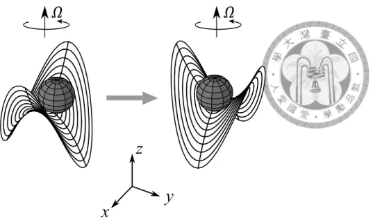
We use a Paul trap to confine the ions [6]. The Paul trap is named after its inventor W. Paul, who won the Nobel Prize in Physics in 1989 for this contribution. From Earnshaw’s theo- rem, we know that a charged particle cannot be captured stably in a static electric field. To circumvent the difficulty, a Paul trap uses a fast-oscillating quadrupole setting of electrodes, usually in radio-frequency, to offer an effective local trapping potential. The concept of a Paul trap is illustrated in Figure 1.1: Intuitively, under the quadrupole saddle-shaped potential surface shown in the left panel, a particle near the saddle point is supposed to move toward the potential minimum along the x axis but fall off along the y axis for the potential is a local maximum. But before the particle gets to leave the trap, the potential surface rotates about the z axis such that the potential along the y axis becomes a local minimum, as shown in the right panel, and pushes the particle back to the saddle point.

As a consequence, the charged particle can be effectively confined as long as the rotating frequency of the quadrupole surface is appropriately chosen.

Figure 1.2 shows the schematic figure of a linear Paul trap, which is typically formed by 4 parallel wires. In Figure 1.2(a), two diagonal electrode wires are applied RF voltages, which yield an instantaneous potential ΦRF = ^V⁰^{cos Ωt}₂ (1 + ^x²_R^−y2²) (R is a geometrical factor). Its time-averaged value is U_eff = ¹₂mω_r²(x² + y²), where ω_r = √ ^eV⁰

2mΩR², m is the mass and e is the charge of a single ion [18]. The other two wires are segmented into different DC voltages along the z direction such that a local DC potential Φ_DC =

κU0

2z₀²(z²− ¹₂(x²+ y²)) (κ, z₀ are geometrical factors) can be built to provide confinement along the wires. Combining the DC and RF parts, the effective potential energy in 3-

(16)

�

x

y z

�

Figure 1.1: The analogous figure of Paul trap. A particle is confined in a rotating saddle- shaped potential surface.

dimension can be approximated by

U = 1

2mω_x²x²+ 1

2mω²_yy²+1

2mω_z²z²,

where ω_z = √

eκU0

mz₀², and ω_x = ω_y =

√

ω_r²− ¹₂ω²_z. Typically, ω_x,y is much larger than ω_z to make the ions aligned along the z axis. For recent development of the ion trap, some groups have started to construct ion traps on surfaces (Figure 1.2(b)) [19] for its advantages on easy fabrication, good accessibility, and simple electronic circuit design.

(a)

DC RF

(b)

y

x z

RF DC

Figure 1.2: The schematic figure of an ion trap device. (a) The standard Paul trap formed by four parallel wires. (b) The surface-electrode ion trap [19].

(17)

1.3 Universal quantum gate

Any quantum circuit can be decomposed into single-qubit rotation gates and two-qubit entangling gates, e.g. control-NOT (CNOT) gates or control-phase-flip (CPF) gates [20].

This is called the universality of the quantum gates. In this section, we will discuss how to implement the universal gates with the trapped ions.

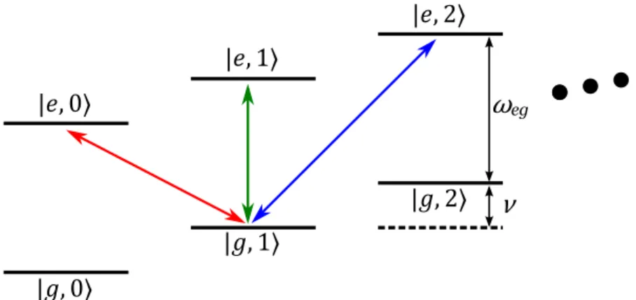
Suppose the information is encoded in an ion’s hyperfine state |g⟩ (ground state) and

|e⟩ (excited state). The energy separation between the two levels is ¯hωeg. Consider a vibrational mode in a harmonic trap with an angular frequency ν, which can be described by the Fock basis|n⟩. The energy configuration of the joint states of an ion is shown in Figure 1.3.

ω_eg

ν

|�, 0⟩

|�, 1⟩

|�, 2⟩

|�, 0⟩

|�, 1⟩

|�, 2⟩

Figure 1.3: The energy level of a trapped ion. The green, blue, and red arrows correspond to the carrier, blue sideband and red sideband transitions respectively.

We now apply laser beams to drive transitions between these states. The Hamiltonian of the laser-ion interaction in the interaction picture reads [21]

H_I = ¯hΩσ⁺e^{−i(δt−ϕ)}exp(

iη(ae^−iνt+ a^†e^iνt))

+ H.c., (1.1)

where Ω is the Rabi frequency of the laser, δ = ω− ωegis the laser-ion detuning, ϕ is the phase offset of the laser. σ⁺ = |e⟩⟨g| and σ⁻ =|g⟩⟨e| are raising and lowering operators of the atomic states; a and a^†are annihilation and creation operators of the phonon states;

η = k

√

¯ h

2mν is the Lamb-Dicke parameter with k the wavevector of the laser. The Lamb- Dicke parameter characterizes the ratio between the oscillation amplitude of the ion to

(18)

the wavelength of the laser. Taking the Lamb-Dicke limit η√

n ≪ 1, which means the displacement of the ion is much smaller than the wavelength so that it does not feel the spatial dependence of the field, the Hamiltonian becomes

H_I = ¯hΩ{σ⁺e^{−i(δt−ϕ)}+σ⁻eî(δt−ϕ)+iη(σ⁺e^{−i(δt−ϕ)}−σ⁻eî(δt−ϕ))(ae^−iνt+a^†eîνt)}. (1.2)

Now we discuss the three cases of interest: δ = 0, and δ = ±ν in the following, where we ignore the fast oscillating terms:

1. For δ = 0 (carrier transition, shown by the green arrow in Figure 1.3), the laser couples|g, n⟩ and |e, n⟩. The Hamiltonian is

H = ¯hΩ(σ⁺e^iϕ+ σ⁻e^−iϕ). (1.3)

2. For δ = ν (blue sideband transition, shown by the blue arrow in Figure 1.3), the laser couples|g, n⟩ and |e, n + 1⟩. The Hamiltonian is

H = i¯hΩη(σ⁺a^†e^iϕ− σ⁻ae^−iϕ), (1.4)

and we get the effective Rabi frequency

Ω_n,n+1 =√

n + 1ηΩ. (1.5)

3. For δ = −ν (red sideband transition, shown by the red arrow in Figure 1.3), the laser couples|g, n⟩ and |e, n − 1⟩. The Hamiltonian is

H =−i¯hΩη(σ⁺ae^iϕ− σ⁻a^†e^−iϕ), (1.6)

and the effective Rabi frequency is

Ω_n,n₋₁ =√

nηΩ. (1.7)

(19)

When we set δ = 0, the evolution of the states is

|en⟩ → cos(_θ

2

)|en⟩ − i sin(_θ

2

)e^iϕ|gn⟩

|gn⟩ → −i sin(_θ

2

)e^−iϕ|en⟩ + cos(_θ

2

)|gn⟩ , (1.8)

where θ = Ωτ , with the laser pulse duration τ . By tuning the duration time and the phase offset of the laser pulse, the single-qubit rotation can be achieved.

For a two-qubit gate, we use vibration as the quantum bus to communicate two qubits.

At the beginning and the end of the operation, the internal states and the motional states are desired to be disentangled. In the following subsections, we will discuss three types of the two-qubit gates.

1.3.1 Cirac-Zoller gate

The first two-qubit gate operation of ion trap was proposed by J. I. Cirac and P. Zoller in 1995 [8]. It requires the motional mode to be cooled to the ground state|n = 0⟩. The scheme has three steps, as illustrated in Figure 1.4.

1. Shine a laser beam with detuning δ =−ν on the mth ion. The laser couples |e⟩_m|0⟩

and|g⟩_m|1⟩. The evolution of the states is given by

|e0⟩ → cos(_θ

2

)|e0⟩ − i sin(_θ

2

)e^iϕ|g1⟩

|g1⟩ → −i sin(_θ

2

)e^−iϕ|e0⟩ + cos(_θ

2

)|g1⟩ , (1.9)

where θ = Ω_1,0τ , with the effective Rabi frequency Ω_1,0 = ηΩ (see Equation (1.7)).

Setting ϕ = 0 and θ = π (π-pulse), if the mth ion is at |g⟩_m initially, the state remains unchanged. If the mth ion is at |e⟩_m initially, the population is driven to

|g⟩_m|1⟩ and gains a phase −i (see Equation (1.9)).

3. Apply again a π-pulse with δ = −ν and ϕ = 0 on the mth ion to take the phonon

(20)

state back to|0⟩.

|�⟩_�|0⟩

|�⟩_�|1⟩

|�⟩_�|0⟩

|�⟩_�|1⟩

|�⟩_�|0⟩

|�⟩_�|1⟩

|�⟩_�|0⟩

Step 1: on mth ion Step 2: on nth ion Step 3: on mth ion

Figure 1.4: The concept of the Cirac-Zoller gate.

The overall evolution of the states then becomes

|g⟩_m|g⟩_n|0⟩ → |g⟩_m|g⟩_n|0⟩ → |g⟩_m|g⟩_n|0⟩ → |g⟩_m|g⟩_n|0⟩

|g⟩_m|e⟩_n|0⟩ → |g⟩_m|e⟩_n|0⟩ → |g⟩_m|e⟩_n|0⟩ → |g⟩_m|e⟩_n|0⟩

|e⟩_m|g⟩_n|0⟩ → −i |g⟩_m|g⟩_n|1⟩ → i|g⟩_m|g⟩_n|1⟩ → |e⟩_m|g⟩_n|0⟩

|e⟩_m|e⟩_n|0⟩ → −i |g⟩_m|e⟩_n|1⟩ → −i |g⟩_m|e⟩_n|1⟩ → − |e⟩_m|e⟩_n|0⟩

.

(1.10) Define|g⟩ = |0⟩ and |e⟩ = |1⟩, then we get the CPF gate. Because the effective Rabi frequency Rabi frequency Ω_n,n₋₁ is different with different phonon state|n⟩, we need to cool the motional state to the ground one|n = 0⟩.

Cirac-Zoller gate was first realized by Schmit-Kaler et al. in 2003 [22].

1.3.2 Mølmer-Sørensen gate

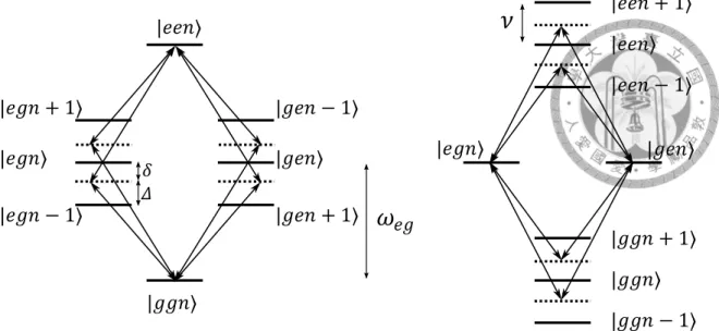
K. Mølmer and A. Sørensen proposed the gate scheme that can be operated in thermal motion [9]. In this scheme, we apply bichromatic laser beams on both ions. The laser frequencies are ω_eg ± δ, which are close to the blue and red sidebands, respectively. The energy levels and the transition paths are shown in Figure 1.5.

In the weak-field regime ηΩ ≪ ν − δ, the phonon number n only changes by ±1.

(21)

� �

|��⟩

|�� − 1⟩

�

_��

|��⟩

|�� + 1⟩ |�� − 1⟩

|��⟩

|�� + 1⟩

�

|��⟩ |��⟩

|��⟩

|�� + 1⟩

|�� − 1⟩

|�� + 1⟩

|�� − 1⟩

Figure 1.5: The concept of the Mølmer-Sørensen gate. Bichromatic laser beams are applied on the ions. The intermediate states are not populated because of the off resonance.

The overall transitions are|ggn⟩ ↔ |een⟩ (left panel) and |egn⟩ ↔ |gen⟩. These paths interfere destructively and eliminate the dependence of phonon number n [10].

In the left panel of Figure 1.5, the path |ggn⟩ ↔ {|egn ± 1⟩ , |gen ± 1⟩} ↔ |een⟩ is the cascade-type Raman transition with multi intermediate levels. Since the intermediate states do not fulfill the resonance condition, these states are not populated in the process.

The evolution is then

|een⟩ → cos(_e

Ωτ 2

)|een⟩ + i sin(_e

Ωτ 2

)|ggn⟩

|ggn⟩ → i sin(

Ωτe 2

)|een⟩ + cos(

Ωτe 2

)|ggn⟩ , (1.11)

with the effective Rabi frequency

eΩ =∑

m

Ω_nmΩ_mn

∆_m , (1.12)

where m denotes the intermediate states|eg ± 1⟩ and |ge ± 1⟩, Ωnm(Ω_mn) is the effective Rabi frequency driving|ggn⟩ ↔ |m⟩ (|m⟩ ↔ |een⟩) (shown in Equation (1.5) and (1.7)), and ∆m = ωm − (Em − Eggn) with ωm the laser frequency driving |ggn⟩ ↔ |m⟩ and (E_m− Eggn) the energy spacing between|m⟩ and |ggn⟩.

We get

eΩ = η²Ω²

ν− δ, (1.13)

(22)

which is independent of the phonon number n. The independence of n is because the transitions|ggn⟩ ↔ {|egn − 1⟩ , |gen − 1⟩} ↔ |een⟩ gives a factor of n, and the transition|ggn⟩ → {|gen + 1⟩ , |egn + 1⟩} ↔ |een⟩ gives a factor of n + 1. These paths have opposite detunings, eliminating the dependence of n. As a result, the Mølmer-Sørensen gate can be operated when the phonon state is under thermal distribution. K. Mølmer and A. Sørensen also showed that this gate scheme has high fidelity even during heating.

Similarly, The evolution in the right panel of Figure 1.5 is

|gen⟩ → cos (_e

Ωτ 2

)|gen⟩ − i sin(_e

Ωτ 2

)|egn⟩

|egn⟩ → −i sin(

Ωτe 2

)|gen⟩ + cos(

Ωτe 2

)|egn⟩ , (1.14)

with the same effective Rabi frequency eΩ shown in Equation (1.13).

Setting eΩτ = π/2, we get the maximal entanglement of the qubits. Combining with single-qubit rotation, we can achieve CNOT gate.

The experiment of the the Mølmer-Sørensen gate was first realize by C. Sackett et al. in 2000 [23]. In 2011, T. Monz et al. created 14-qubit entanglement by using this gate scheme [24].

1.3.3 Geometrical phase gate

K. Mølmer and A. Sørensen also proved that their gate scheme can be achieved without the restriction of being in the weak-field regime [10]. A similar idea was proposed indepen- dently by G. Milburn et al. in 2000 [25]. In Milburn’s scheme, we apply spin-dependent forces on the ions, and drive clockwise or counterclockwise trajectories in the phase space depending on the internal states. At the end of the gate operation, the ions return to the original motional state, obtaining a phase which equals to the area of the close loop.

To study the effect of a spin-dependent force, first we consider a forced oscillator. For an oscillator with an angular frequency ν pushed by a force F sin ωt, the Hamiltonian in the interaction picture is [26]

H = F x₀(ae^iδt+ a^†e^−iδt), (1.15)

(23)

where δ = ω− ν, and x0 =√

¯

h/(2mν). The evolution operator of the forced oscillator is [26]

U (τ ) = e^{iϕ(τ )}D(α(τ )), (1.16) where D(α) = e^αa^†^−α^∗^ais the displacement operator with α(τ ) = −_¯_hⁱ ∫_τ

0 F x₀e^iδtdt, and ϕ(τ ) = Im{∫τ

0 α^∗dα} .

The additional phase ϕ can be understood by the the relation of displacement ope- rator D(α + β)e^{i Im}^{α^∗^β^} = D(α)D(β). Equation (1.16) can be regraded as a series of infinitesimal displacement.

After a period τ = 2π/δ, the displacement operator D(α) = 1 makes the motional state back to the origin, and the state gains a phase ϕ which equals to the area of the closed loop.

For spin-dependent forces acting on the ions, the Hamiltonian is

H =∑

i

F x0(ae^iδt+ a^†e^−iδt)σ^z_i, (1.17)

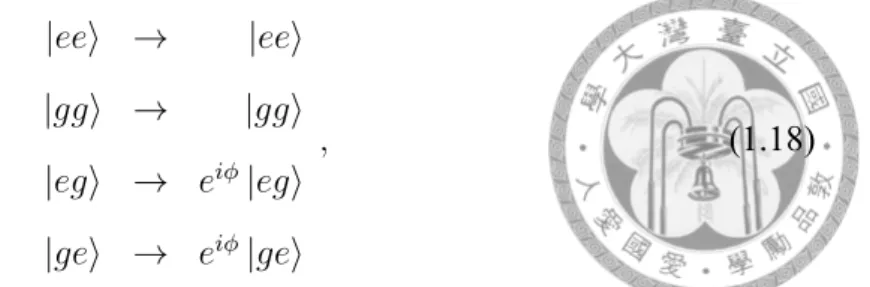
where σ^z_i =|e⟩⟨e| − |g⟩⟨g| is the Pauli matrix, and the subscript i = 1, 2 denotes the ion’s index. Equation (1.17) shows that the ion feels a force F when the internal state is|e⟩, and−F when the internal state is |g⟩. When both ions are at the same internal states (|ee⟩

or|gg⟩), the ions move back and force together (center-of-mass mode). When the two ions have different internal states (|eg⟩ or |ge⟩), the ions move in the opposite directions (breathing mode). Consider that only the breathing mode is excited by applying the laser with frequency close to the mode frequency. If the ions’ internal state is|ee⟩ or |gg⟩, it remains unchanged. If the ions’ internal state is|eg⟩ or |ge⟩, the motional state displaces in the phase space.

When the ions’ motional state goes back to the origin, the evolution of the internal

(24)

states is described by

|ee⟩ → |ee⟩

|gg⟩ → |gg⟩

|eg⟩ → e^iϕ|eg⟩

|ge⟩ → e^iϕ|ge⟩

, (1.18)

which is illustrated in Figure 1.6. By choosing appropriate laser frequency and intensity, we can make ϕ = π/2. Then Equation (1.18) is equivalent to the CFP gate up to single- qubit rotation. The experiment of the geometrical phase gate is realized by Leibried et al. in 2003 [27].

x p

|��⟩ → �^��|��⟩

Figure 1.6: The concept of the geometrical phase gate. If the ions’ internal state is|eg⟩ or

|ge⟩, the motional state displaces in the phase space. At the end of the gate operation, the motional state goes back to the origin and gains a phase corresponding to the area of the closed loop.

1.4 Transverse-mode scheme

S.-L. Zhu and L.-M. Duan proposed to implement gates that employs the transverse motional modes instead of the traditional way with longitudinal modes [28]. The advantage of doing so is that the transverse confinement is usually much stronger than the longitudinal one so that, under the same temperature, the number of transverse phonons can be drastically suppressed, making the high-fidelity quantum gates rather robust against temperature. Further, since the transverse trapping frequency determines the highest motional

(25)

energy scale, other collective motion (longitudinal one, or dipole-dipole-like interaction from neighbors) are considered slow compared to the transverse dynamics. Therefore, every ion’s transverse motion can be viewed as individual independent oscillation. This point of view allows us to consider only the local modes relevant to the participating ions in a quantum gate. A systematic way of pulse shaping was thus proposed for two-qubit gates whose speed can be made comparable to the transverse trapping frequency, which is of the order of microsecond for the gate time.

1.5 Cooling in trapped ions

In current quantum gate experiments with trapped ions, the ions are usually pre-cooled by Doppler laser cooling down to the order of millikelvin, the level so-called the Doppler temperature T_D = ¯hγ/(2k_B), with γ the natural linewidth of the atomic state. To further go below this limit, the method of resolved sideband cooling is utilized. The idea is via the optical pumping technique by driving the red-sideband transition: Consider an trapped ion initially lies in its atomic ground state but a highly excited motional state characterized by the phonon number n. A laser beam resonant with the red-sideband transitions is applied on this ion, taking it to its atomic excited state while the phonon number is lessen by one.

Next, due to spontaneous relaxation, the ion de-excites back to its ground state with the motional state of a smaller phonon number n− 1. By repeating such procedures, one can cool the system nearly to its ground state [29].

However, this method might not be easily generalized to large-scale ion arrays. The main obstacle is the increasing number of motional modes. A specific red-sideband laser is needed for each mode, which becomes impractical when more ions are added. In Refe- rence [28, 30], it has been shown that the transverse-mode proposal does not require the stringent temperature requirement as the longitudinal one does. Instead, Doppler cooling suffices in the transverse scheme due to the strong confinement and hence low phonon numbers.

Such convenience does not guarantee sufficient cooling in the large-scale ion array considering the gate fidelity. The cooling issue remains with the longitudinal motion,

(26)

which still plays a role that potentially degrades the gate fidelity. The major source of er- ror originates from the finite beam size of the control laser, for which its spatial variation of the field profile can be seen by ions moving longitudinally. In order to build a long array compatible with single ion addressability, the ion spacing must be kept nearly constant. This cannot be done by a simple harmonic trap, where the ion spacing near the trap center is squeezed every time an ion is added, unless the global axial trapping frequency is lowered accordingly. However, lower longitudinal frequency means the associated motion is more difficult to be cooled and hence more sensitive to temperature. This indeed sets a serious challenge for the large-scale ion trap quantum computation with the linear Paul trap configuration.

In this work, we propose to use optical tweezers that effectively pin some of the ions, introducing extra local traps to the system. To be more specific, we plan to apply optical tweezers used like partitions so that each “compartment” can be seen as a smaller ion trap.

We will test the idea by looking mainly at the mode frequencies and the cooling efficiency.

1.6 Thesis outline

The thesis is organized as follows. In Chapter 2, we will discuss the collective motion in an ion trap. We further look at the effects of the collective motion when optical tweezers are applied regularly along the ion chain. In Chapter 3, we will discuss sympathetic cooling in the ion trap. We continuously cool some of the ions and find the temperature distribution of the ion chain, and compare the results with and without optical tweezers. We also study the relaxation dynamics of the ions as indication of cooling. Finally, we conclude our work in Chapter 4.

(27)

Chapter 2 Collective motion of trapped ions with optical tweezers

2.1 Overview

An ion trap confines N ions with the trapping frequency ω_x, ω_y, and ω_zalong the x, y, and z directions, respectively. Typically, ω_x = ω_y, and ω_x(y) ≫ ωz so that all the N ions are aligned along the z axis. As more ions are added in the trap, the “inner” ions are pushed closely by the “outer” ones, causing the spacing around the trap center to decrease. To keep a certain distance between ions for individual laser addressing, we need to reduce the trapping frequency ωz as N grows. Meanwhile, it is however more difficult to cool lower frequency phonon modes. This can be seen from the estimated phonon number

¯

n∼ kBT /(¯hω). To overcome this problem, we test the idea by applying optical tweezers on the ions [15], which are arranged regularly along the chain as shown in Figure 2.1.

By raising the tweezer frequency for local ions, the collective mode frequency will be enhanced by a few times. This will not only help phonon removal, but also set a frequency bound in a linear large-scale array, where the potential bottom of a traditional Paul trap is nearly flat.

(28)

x z

y optical tweezer optical tweezer optical tweezer optical tweezer

Figure 2.1: Optical tweezers are applied on the ions (nodes), who are arranged periodically on the chain.

2.2 Normal modes of the harmonic trap

For N ions in the Paul trap, the overall potential including their Coulomb interaction reads

U =

∑N i

1

2mω_x²x²_i + 1

2mω²_yy_i²+1

2mω_z²z_i²+

∑N i

∑

j<N

e² 4πϵ₀

1

|Ri− Rj|, (2.1)

where R_i is the position of the ith ion. The equilibrium position z_i⁰ of the ith ion can be found by solving ∂U /∂z_i = 0. For convenience, we define a length unit z_s = (_4πϵ^e²

0mω²_z)^1/3. Figure 2.2 shows the equilibrium positions of ions in units of z_sby keeping the trapping frequency ω_z fixed for N = 1∼ 10.

We can see that the closest ions are at the center of the chain. The minimum spacing d0between ions become small as the number of ions N grows (shown in the dotted line).

A numerical result of the separation of central ions as function of N is given by d₀ ≈ 2z_sN^−0.57 [31], and for N ≫ 1, d0 ∼ zs(ln(N )/N²)^1/3) [32].

To find the normal modes, we do Taylor expansion around the equilibrium and get U ≈ U0+∑

ξ,ξ^′,i,j 1

2A^ξξ_ij^′∆x^ξ_i∆x^ξ_j^′, where ∆x^ξ_i is the displacement of the ith ion along the ξ = x, y (transverse) and ξ = z (longitudinal) directions with respect to its equilibrium position, and A_ij = ^∂²^U

∂x^ξ_i∂x^ξ′_j

0

(

0denotes ions at equilibrium positions) forms the coupling matrix. Here U0 denotes the potential constant at the equilibrium but is not important.

Because x⁰_i, y_i⁰ = 0, only _∂x^∂²^U

i∂xj

0

, _∂y^∂²^U

i∂yj

0

, and _∂z^∂²^U

i∂zj

0

survives. This suggests that the

(29)

motion along the x, y, and z directions is decoupled. We then have

A^ξ_ij =









mω_ξ²+∑N

j=1, j̸=i e² 4πϵ0

aξ

|^zⁱ⁰^−z⁰^j|³ , i = j

−_4πϵ^e²₀|^z⁰i−z^a^ξ_j⁰|³ , i̸= j (2.2)

where a_x(y) =−1 and az = 2 [28]. The mode frequencies ωξ,kand the mode functions b^ξ,k_i of the kth mode can be found by solving the eigenvalue equation∑

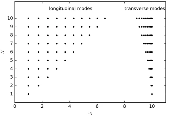
jA^ξ_ijb^ξ,k_j = mω_ξ,k² b^ξ,k_i . The mode frequencies for N = 1 to 10 are shown in Figure 2.3. Here we set ω_x(y) = 10ω_z, and choose ω_z as the frequency unit. For the longitudinal modes (motion along the z direction), the lowest frequency corresponds to the center-of-mass mode, for which every ion moves back and forth all together. Therefore the mode frequency of this mode is exactly equal to the trapping frequency ω_z. On the contrary, for the transverse motion (along the z direction) the center-of-mass mode has the highest frequency. It can be ob- served that typically the transverse modes have higher and narrower spectral distribution than the longitudinal ones.

Though we set ω_x(y)/ω_z the same value when N = 1 to 10 in Figure 2.3. The ratio ω_x(y)/ω_z should be increased to keep the ions perfectly aligned when N gets very large.

The criterion of a linear array configuration is approximated by ω_x(y)/ω_z > 0.73N^0.86 [32], and for N ≫ 1, ωx(y)/ω_z > 0.77N /√

ln N [33].

2.3 Normal modes when applying optical tweezers

Optical tweezers are dipole forces that can be formed by focused Gaussian beams incident on an atom. Suppose a laser beam is incident on a target ion from the y direction, which is perpendicular to the axis of the ion chain. When the field is largely detuned, it introduces a tweezer potential

U = 2U0

w₀² (x² + z²)

(30)

where U0 =−_ck^3γP3w₀²δ with γ the natural linewidth, δ < 0 corresponding to red detuning, k, w₀, P are the wavenumber, beam size, power of the laser, respectively. Here we ignore the y direction term because the transverse confinement of a Paul trap is typically much stron- ger than the axial trapping provided by a Gaussian tweezer beam along the y direction. By applying optical tweezers on some of the ions (called pinned ions), we effectively change the local frequencies experienced by the pinned ions, i.e., ω_z(x),i → ωz(x),i = ω_z(x) + ω_ot. Then we have a new matrix A^z(x) and new eigenfrequencies ω_z(x),k.

Figure 2.4 shows the mode frequencies of 13 ions given different numbers of optical tweezer beams. We set ω_x = 10ω_z, and choose ω_z as the frequency unit. The subfigures (a), (c), (e), and (g) correspond to the longitudinal mode, and (b), (d), (f), and (h) the transverse mode. The optical tweezers are arranged periodically. The period for pinned ions are 12, 6, 4, and 3 for the subfigure (a)(b), (c)(d), (e)(f), and (g)(h), respectively. In other words, the indices of pinned ions in the subfigure (a) and (b) are i = 1 and 13; i = 1, 7 and 13 in (c) and (d); i = 1, 5, 9 and 13 in (e)and (f). i = 1, 4, 7, 10 and 13 in (g) and (h).

For a small optical tweezer frequency, the eigenfrequencies grow as ωot increases. Note that when ω_ot keeps increasing, the eigenfrequencies of N_p modes grows like ω_z(x)+ ω_ot where N_pdenotes the number of pinned ions. The other N−Npeigenfreqencies, however, approach to fixed values in the limit of large ω_ot. The reason why these frequencies are bounded is that, as ω_ot gets large, the ”pinned ions” act more like a fixed one, leaving N− Np degrees of freedom.

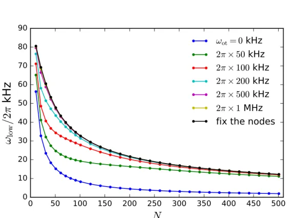
We calculate the lowest mode frequency ω_lowof the ion chain with different N when applying optical tweezers regularly on one of every 10 ions. As an example, we choose

171Yb⁺ions and see how the lowest frequency scales with increasing number of ions while keeping the minimum separation d₀ = 10 µm. The result is shown in Figure 2.5. We find for a typical ion trap that contains a few tens of ions, even though the application of tweezers does raise the lowest mode frequency, its value is mainly determined by the trapping frequency. However, as more and more ions are added and the global trap gets shallower, the effect due to optical tweezers becomes more and more dominant. On the other hand, the enhancement of the lowest frequency has an upper bound as the tweezer

(31)

strength increases. Explicitly, we compare the lowest mode in the two cases of strictly fixing the end ions in space and “optical pinching” the end ions by frequency 2π× 500 kHz. We find that the deviation of the frequency between these two cases is within 1%.

This suggests that the pinned ions set potential “walls” for other ions. Most importantly, it can be seen that, without tweezers, the lowest mode approaches to zero frequency in the limit of a large-scale array. The zero-frequency mode is equivalent to pure translation, and is extremely hard to be cooled for charged particles. By means of optical tweezers, the longitudinal fundamental frequencies are provided by pinned ions. This feature does not depend on the global trap and is thus scalable.

(32)

3 2 1 0 1 2 3

z

1 2 3 4 5 6 7 8 9 10

N

Figure 2.2: The equilibrium position of ions. The length unit is z_s. The dotted line shows the separation between central ions decreases as number of ions increases [31].

0 2 4 6 8 10

ω

k

1 2 3 4 5 6 7 8 9 10

ω

ot 0

2 4 6 8 10

ω

z k

(g) # of pinned ions = 5

0 5 10 15 20

ω

ot 8.0

8.5 9.0 9.5 10.0 10.5 11.0 11.5 12.0

ω

x k

(h) # of pinned ions = 5

Figure 2.4: The (a)(c)(e)(g) longitudinal and (b)(d)(f)(h) transverse mode frequencies of 13 ions applied by optical tweezers periodically with the tweezers period (a)(b) 12, (c)(d) 6, (e)(f)4, and (g)(h)3.

(34)

0 50 100 150 200 250 300 350 400 450 500

N

0 10 20 30 40 50 60 70 80 90

To overcome the challenge of construction, we propose to assemble small ion arrays into a long one. By controlling the DC voltages that provide the longitudinal potential, one can realize many local minima each of which can be considered as a small ion trap.

Similar to the ion shuttling proposal, small arrays can be moved and merged by varying the voltages. But, at this stage, ions have not yet contained quantum information. The Doppler cooling laser can be still on to stabilize the ion array.

When the length of the ion chain becomes large, the majority of ions sits at the flat bottom of the potential. Coulomb interaction from both sides cancels out as long as ions

(36)

are distributed uniformly. Under this condition, we propose to use optical tweezers that pin the ions in space. The optical tweezers provide local trapping frequencies, which can help stabilize the linear structure. By arranging optical tweezers periodically, the length of an ion array can be arbitrarily long in principle.

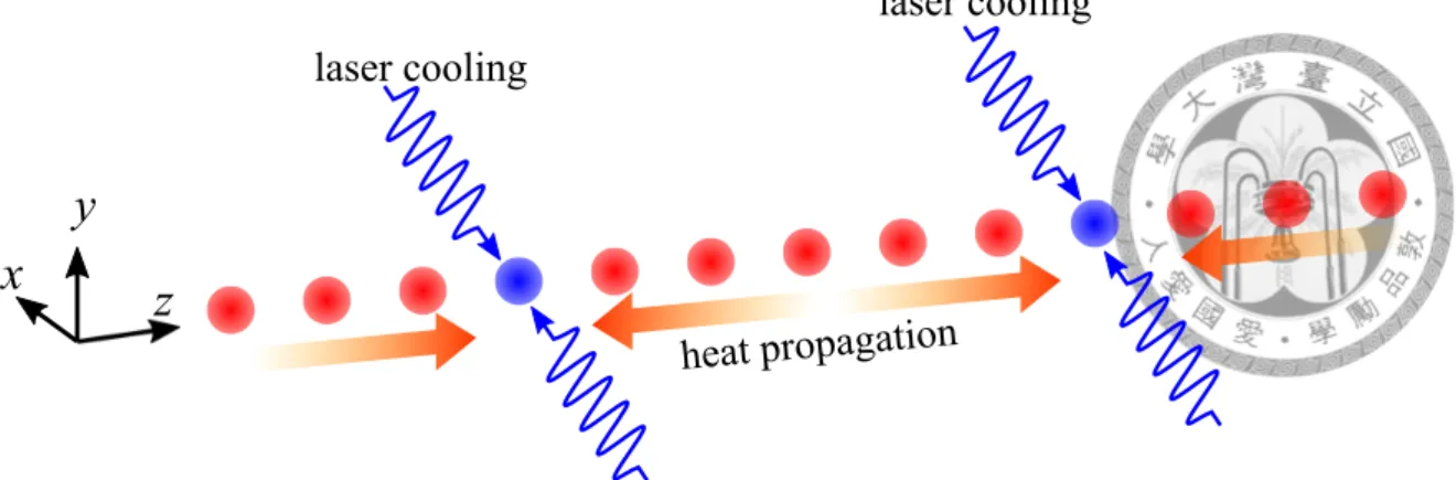
During computing, cooling is still an important issue. Ions will heat due to background noise which is induced by, for example, the fluctuation of voltage of the electrodes and micromotion [34]. G.-D. Lin et al. showed that a high-fidelity gate can be achieved at Doppler temperature by using the transverse-mode gate operation [28, 30]. For long-time gate processing, we should apply laser cooling continuously to maintain the ion chain at such a low temperature. However, an ion which is Doppler cooled can not participate in quantum computation because its qubit state will be destroyed repeatedly during the cooling process. The solution to this problem is via sympathetic cooling [16]. Under sympathetic cooling, a subset of ions (cooling ions) are laser cooled continuously and play the role of “heat drain”. The motional occupation of other ions (qubit ones) will decrease through heat exchange (due to Coulomb interaction) between ions (Figure 3.1).

G.-D. Lin et al. showed that in principle we can cool a large ion crystal efficiently by arranging the cooling ions periodically [17].

In this chapter, we discuss the ions’ motion under sympathetic cooling associated with optical tweezers. First, we show the motional steady state of ions when arranging laser cooling and optical tweezers periodically. Then, we apply optical tweezers on just two chosen ions that contain two computational ions in between. Finally, we study the associated relaxation dynamics and find the timescale of heat equilibration.

3.2 Model

We will discuss the motion of the ions in this section. Assume that each ion couples to an individual heat bath, which depends on laser cooling or background heating. Besides the harmonics potential and the Coulomb force, a random kick due to background noise also acts on the ion. The motion of ions are described by the Heisenberg-Langevin equation

以光鑷與協同冷卻實現可擴展的離子阱量子電腦

Department of Physics College of Science

National Taiwan University Master Thesis

誌謝

摘要

Abstract

Contents

List of Figures

Chapter 1 Introduction

1.1 Motivation

1.2 Paul trap

�

x

y z

�

1.3 Universal quantum gate

1.3.1 Cirac-Zoller gate

1.3.2 Mølmer-Sørensen gate

�

�

1.3.3 Geometrical phase gate

1.4 Transverse-mode scheme

1.5 Cooling in trapped ions

1.6 Thesis outline

Chapter 2

Collective motion of trapped ions with optical tweezers

2.1 Overview

2.2 Normal modes of the harmonic trap

2.3 Normal modes when applying optical tweezers

3 2 1 0 1 2 3

z

1 2 3 4 5 6 7 8 9 10

N

0 2 4 6 8 10

ω

1 2 3 4 5 6 7 8 9 10

N

longitudinal modes transverse modes

ω

ω

ω

ω

ω

ω

ω

ω

ω

ω

0 50 100 150 200 250 300 350 400 450 500

N

0 10 20 30 40 50 60 70 80 90

ω lo w / 2 π kH z

ω

= 0 kHz

2 π

50 kHz

2 π

100 kHz

2 π

200 kHz

2 π

500 kHz

2 π

1 MHz fix the nodes

Chapter 3

Sympathetic cooling for large-scale computing

3.1 Overview

3.2 Model