國立臺灣大學理學院心理學研究所 碩士論文
Graduate Institute of Psychology College of Science
National Taiwan University Master Thesis
以小鼠探討紋狀體不同腦區在增強學習 以及酬賞預測誤差中所扮演的角色
The Role of Striatal Subregions in Reinforcement Learning Process and Reward Prediction Error using
Excitotoxic Lesion in Male Mice
劉雅文 Ya-Wen Liu
指導教授:賴文崧 博士 Advisor: Wen-Sung Lai, Ph.D.
中華民國 104 年 1 月
January, 2015
i
摘要
紋狀體分屬於基底核,是主要接收基底核訊息的腦區,更參與動作控制 和酬賞相關的學習。近來的研究指出紋狀體與行動值以及酬賞預測誤訊號 (個體 預期得到的酬賞和實際得到的酬賞之差異)的更新有關。紋狀體可進一步分成三 個分區,各分區分別與不同種類的學習歷程有關。背內側紋狀體主要接收來自關 聯皮層的訊息、與目標導向的行為學習有關;背外側紋狀體主接收來自感覺動作 皮層的訊息、與習慣學習有關;伏隔核則被認為是表徵對未來酬賞預期的重要腦 區,並可根據此預期進一步影響酬賞導向的行為選擇。然而,紋狀體內各分區在 增強學習以及酬賞相關的學習中所扮演的角色、及其內在機制仍未有一定論。所 以,本研究的目的為檢視不同的紋狀體分區在增強學習、酬賞預測誤訊號更新所 扮演的角色,使用興奮性毀壞藥物注射紋狀體不同分區搭配二選項動態酬賞作業,
觀察毀壞後小鼠的學習行為是否改變。本研究使用的二選項動態酬賞作業包含兩 組不同的酬賞機率學習,小鼠的每次選擇都會被記錄。我們使用增強學習模型來 分析資料,酬賞預測誤的相關參數估計使用貝氏估計法,另使用配對法則分析小 鼠的選擇行為傾向。本研究結果顯示,背內側紋狀體毀壞小鼠在整個學習過程裡,
相較於控制組小鼠,除了達到預設標準需要更多的選擇次數外,也在學習過程中 累積更多錯誤。背外側紋狀體以及伏隔核毀壞小鼠則沒有展現整體學習行為上的 差異。另使用增強學習模型分析,發現背內側紋狀體以及伏隔核毀壞小鼠皆有酬 賞預測誤訊號更新速度下降、行為選擇一致性些微上升的情況。配對法則分析部 分,沒有發現任何毀壞組及控制組的組間差異。整體而言,本研究證實了背內側
ii
紋狀體的功能損傷會影響酬賞相關學習和行為決策的表現。除此之外,亦證實背 內側紋狀體以及伏隔核對於二選項動態酬賞作業的重要性,以及兩腦區皆在決策 行為的價值評估、行為選擇兩部分扮演重要角色。
關鍵詞:增強學習、酬賞預測誤、紋狀體、興奮性毀壞、二選項動態酬賞作業、
小鼠、決策行為
iii
The Role of Striatal Subregions in Reinforcement Learning Process and Reward Prediction Error using Excitotoxic
Lesion in Male Mice Ya-Wen Liu
Abstract
The striatum is the principal input structure of the basal ganglia that influences motor control and reward-based learning. Emerging studies indicate that it also
contributes to update of action value and reward prediction error (RPE), a discrepancy between the predicted and actual rewards. Previous studies imply that three different subregions of the striatum participating in different kinds of learning processes. The dorsomedial striatum (DMS, also known as “associative striatum” in primates) which receives inputs from the association cortices is implicated in goal-directed behavior in rodents. The dorsolateral striatum (DLS, a part of the sensorimotor striatum in
primates) is related to habit learning in rodents. The nucleus accumbens (NA) is implicated in representing predicted future reward, and the representation can be used to guide action selection for reward. However, the precise role or mechanism of each
iv
subregion in reinforcement learning and reward-based decision making is still under debate. The aim of this study is to examine the role of different striatal subregions (including DMS, DLS, and NA) in reinforcement learning process and reward
prediction error using excitotoxic lesions and 2-choice dynamic foraging task in male C57/Bl6 mice. The 2-choice dynamic foraging task is a risky-choices task which consisted of two kinds of reward ratio learning. The behavioral performance of each of the three lesioned groups and their sham controls were recorded. Their trial-by-trial choice behavior were further analyzed and fit with a standard reinforcement learning model using the Bayesian estimation approach and matching law analysis to elaborate parameters for RPE and reward sensitivity. Compared to sham controls, overall behavioral results indicated that the DMS lesioned mice had more trials to reach the preset criteria and made more cumulated errors during the learning process of this dynamic foraging task. In contrast to the DMS group, both NA and DLS lesioned groups did not exhibited more accumulated trials or more cumulated errors.
Reinforcement learning model analysis further revealed that both DMS and NA lesion mice had a lower learning rate in updating the RPE signaling and a slightly higher perseveration compared to their sham controls. But no significant difference was found in the reward sensitivity among the 3 groups. Collectively, the current study
v
confirmed the importance of DMS and NA in the 2-choice dynamic foraging task and their roles in the value component and choice component of decision making.
Excitotoxic lesion of DMS can significantly impair performance of probabilistic reward-based learning and decision making.
Keywords: reinforcement learning, reward prediction error, striatum, excitotoxic
lesion, 2-choice dynamic foraging task, mice, decision making
vi
Table of Contents
Chapter 1: Introduction ... 1
1. An overview of decision making ... 1
2. A general introduction of reinforcement learning and related models ... 8
3. An overview of striatum: anatomy and neural circuits ... 14
4. The objective of this study ... 21
Chapter 2: Materials and Methods ... 23
1. Animals ... 23
2. Experimental apparatus ... 23
3. Experimental procedures ... 24
4. Data analysis ... 30
Chapter 3: Results ... 37
1. Histology ... 37
2. Behavioral data... 37
3. Matching law analysis ... 41
4. Estimation of learning rate and choice perseveration using reinforcement learning model ... 42
Chapter 4: Discussion ... 45
1. Result summary ... 45
2. DMS lesion mice showed impaired learning of action-outcome association .. 45
3. NA lesion mice only learned slower in more difficult task ... 49
4. The constraint on Bayesian hierarchical model ... 53
5. Motivation control of 2-choice dynamic foraging task ... 54
6. Hierarchical reinforcement learning in the cortico-striatal circuits ... 54
7. Future directions... 57
References ... 59
vii
Tables and Figures
Table 2. 1. The grades of evidence corresponding to values of the Bayes factor ... 80
Figure 2. 1. Schematic diagram of drug injection site. ... 81
Figure 2. 2. The procedure of the 2-choice dynamic foraging task. ... 82
Figure 2. 3. Reinforcement learning model fitting using Bayesian Hierachical estimation. ... 84
Figure 3. 1. The pictures of representative infusion placements in the DLS, DMS and NA... 86
Figure 3. 2. Schematics of coronal section showing the range of acceptable location of infusions within the striatal subregions. ... 89
Figure 3. 3. Total moving distance in open field task. ... 90
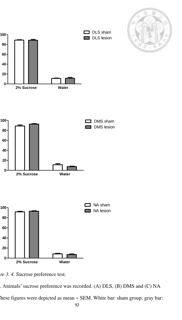
Figure 3. 4. Sucrose preference test. ... 92
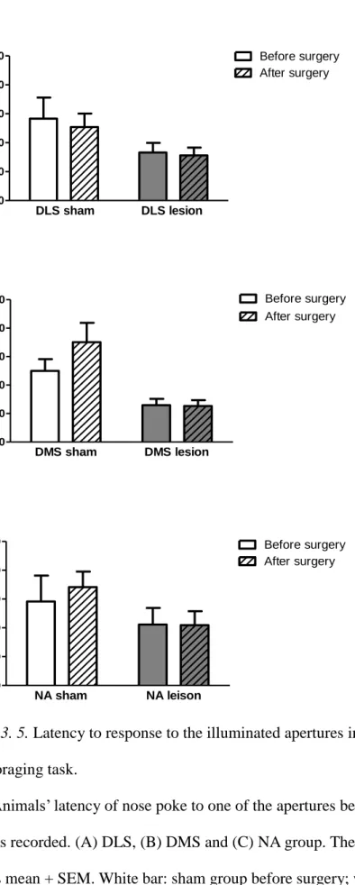
Figure 3. 5. Latency to response to the illuminated apertures in the 2-choice dynamic foraging task. ... 94
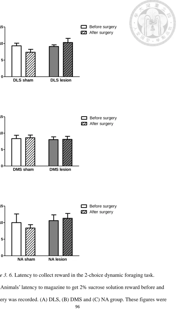
Figure 3. 6. Latency to collect reward in the 2-choice dynamic foraging task. ... 96
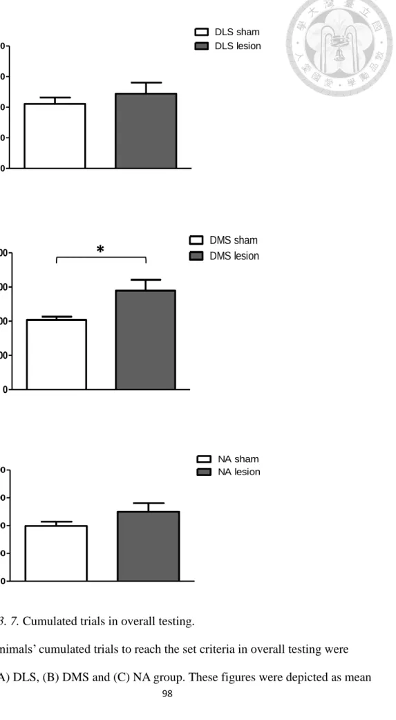
Figure 3. 7. Cumulated trials in overall testing. ... 98
Figure 3. 8. Cumulated trials in 1:3 reward ratio and 1:6 reward ratio learning. ... 100
Figure 3. 9. Cumulated trials in each section of the 2-choice dynamic foraging task. ... 102
Figure 3. 10. Cumulated errors in overall testing. ... 104
Figure 3. 11. Cumulated errors in 1:3 reward ratio and 1:6 reward ratio learning. ... 106
Figure 3. 12. Errors in each section of the 2-choice dynamic foraging task... 108
Figure 3. 13. Steady state choice behavior of all lesion and sham groups. ... 110
Figure 3. 14. The model fitting results of learning rate α. ... 113
Figure 3. 15. The model fitting results of choice perseveration β. ... 115
Figure 3. 16. The Hierarchical reinforcement learning in the cortico-striatal loops. . 116
viii
1
Chapter 1: Introduction
1. An overview of decision making
In everyday life, there are numerous decisions waiting for us, from what food to eat, what clothes to wear, what hair style and what you are going to do in the
future…etc. All of these things need us to make decisions. In short, a decision is a process that weighs priors, evidence, and values of different options to generate a choice intended to achieve particular goals. And this is the main focus of the field of decision making. Recently, a cross disciplinary approach to study decision making process has come out to the mainstream: Neuroeconomics.
Neuroeconomics is a newly established field that integrates the confluence of economics, psychology and neuroscience to the study of decision making to try and create a better model about decisions, interactions, and risks and rewards. Accordingly, neuroeconomics combines the modeling from economics with psychological studies of social and emotional influences on decision making, and utilizes tools from neuroscience that permit the observation of valuation and decision-making
computations that take place in the brain. In the following section, a brief introduction of decision process and its corresponding brain areas are described.
1.1. Elements of a decision. As mentioned, a decision is a process that weighs
2
priors, evidence, and values of different options to generate a choice intended to achieve particular goals. It also can be regarded as a form of statistical inference (Kersten, Mamassian, & Yuille, 2004; Smith, 1961). According to Doya, the process of value-based decision making can be decomposed into four steps (Doya, 2008):
a. Subject identifies the existing situation (or state).
b. Subject evaluates possible options (or actions) according to the reward or punishment every potential choice could bring.
c. Subject makes the final decision after considering own needs.
d. Based on the outcome, subject revaluates the decision.
Although decisions are not always made through these four steps, a standardizing procedure of decision making process is useful in the understanding of how these steps are executed in the brain.
1.2. Brain areas related to value functions. Subject’s internal reward
expectancy represents value functions in decision process. Theoretically, neural signals related to reward expectancy can be divided into two categories: action value and state value (Lee, Seo, & Jung, 2012). Action value functions are useful in
choosing a particular action, especially if such signals are observed before the
execution of a motor response. However, based on the dimension in which choices are
3
made, brain areas related to the corresponding action value functions may vary substantially. In most previous studies, many brain areas are implicated in action value functions, including dorsolateral prefrontal cortex (Barraclough, Conroy, & Lee, 2004; Kim, Hwang, & Lee, 2008), posterior parietal cortex (Dorris & Glimcher, 2004;
Platt & Glimcher, 1999; Sugrue, Corrado, & Newsome, 2004), medial frontal cortex (Seo & Lee, 2009; So & Stuphorn, 2010; Sul, Kim, Huh, Lee, & Jung, 2010),
premotor cortex (Pastor-Bernier & Cisek, 2011), and striatum (Cai, Kim, & Lee, 2011;
Kim, Sul, Huh, Lee, & Jung, 2009; Lau & Glimcher, 2008; Samejima, Ueda, Doya, &
Kimura, 2005; Tai, Lee, Benavidez, Bonci, & Wilbrecht, 2012).
State value functions play a more evaluative role in the brain, and it can be further divided into two categories: pre-decision and post-decision. For the
pre-decision state value functions, researchers found that some of the related brain areas overlapped with the action value functions. Neural activity in the posterior parietal cortex and dorsal striatum showed both characteristics of pre-decision state value functions and action value functions (Cai et al., 2011; Seo, Barraclough, & Lee, 2009; Yang & Shadlen, 2007). Brain areas related to pre-decision state value functions are also found in the ventral striatum (Cai et al., 2011), anterior cingulate cortex (Seo
& Lee, 2007), and amygdala (Belova, Paton, & Salzman, 2008).
4
Post-decision state value functions are also called chosen values, and its related brain areas are also widespread, including orbitofrontal cortex (Padoa-Schioppa &
Assad, 2006; Sul et al., 2010), medial frontal cortex (Sul et al., 2010), ventromedial prefrontal cortex (Hare, Camerer, & Rangel, 2009), dorsolateral prefrontal cortex (Hare et al., 2009), and striatum (Cai et al., 2011; Kim et al., 2009; Lau & Glimcher, 2008). Since the revaluation happens after subjects made their decision, the chosen value may be utilized to revaluate (i.e. compute the difference between the outcome of a choice and the chosen value) and update value functions.
1.3. Brain areas related to action selection. In decision making process, the
action value must be transformed into specific action and corresponding motor structures. Hence, the brain areas involved in action value functions are likely to be related in action selection. Also, brain areas involved in motor control are likely to be related in action selection (Lee, Seo, & Jung, 2012). However, the character of a behavioral task may change the precise anatomical location involved in action selection. For instance, a well-trained motor sequence (fixed stimulus-response association) may rely more on the dorsolateral striatum (Hikosaka et al., 1999; Yin &
Knowlton, 2004, 2006; Yin, 2010), whereas the dorsomedial striatum may be rely
5
more on to perform flexible goal-directed behaviors (Yin, Knowlton, & Balleine, 2005; Yin, Ostlund, Knowlton, & Balleine, 2005). Moreover, recent study using transient optogenetic stimulation of dorsal striatal dopamine D1 and D2
receptor–expressing neurons during decision-making found that the striatal activity is involved in goal-directed action selection (Tai et al., 2012). There are cumulated evidence showing that the lateral intraparietal cortex (LIP) (Roitman & Shadlen, 2002;
Rorie, Gao, McClelland, & Newsome, 2010; Seo et al., 2009), frontal eye field (Ding
& Gold, 2012), and superior colliculus (Horwitz & Newsome, 2001) are involved in selecting a specific physical movement.
In addition, other brain areas may be related to more abstract action selection (Lee, Seo, & Jung, 2012). Action selections like making choices among different objects or goods may rely more on the orbitofrontal cortex (Padoa-Schioppa & Assad, 2006; Padoa-Schioppa, 2011). Compared to the orbitofrontal cortex, the medial frontal cortex may be involved more in action selection guided by endogenous cues (for example, memory) rather than external sensory stimuli. The medial frontal cortex, including the anterior cingulate cortex (Kennerley, Walton, Behrens, Buckley, &
Rushworth, 2006; Lee, Rushworth, Walton, Watanabe, & Sakagami, 2007; Shidara &
Richmond, 2002) and supplementary motor area (Okano & Tanji, 1987; Sohn & Lee,
6
2007; Soon, Brass, Heinze, & Haynes, 2008; Sul, Jo, Lee, & Jung, 2011), may integrate the information about the costs and benefits of particular behaviors and take action. Furthermore, it has been proposed that the anterior cingulate cortex might play a more important role in selecting an action voluntarily and monitoring its outcomes (Kennerley et al., 2006; Quilodran, Rothé, & Procyk, 2008; Rushworth, Walton, Kennerley, & Bannerman, 2004).
1.4. Neural mechanisms for updating value functions. Value updating
functions can be divided into two parts. First, subjects need to relate an action to its corresponding outcome correctly. Deficit of this function could interfere with the process of updating value functions suitably. Previous studies showed that subjects
with lesions in the orbitofrontal cortex are impaired in reversal learning tasks (Fellows
& Farah, 2003; Murray, O’Doherty, & Schoenbaum, 2007; Schoenbaum, Nugent,
Saddoris, & Setlow, 2002), and the deficits produced by the lesions were due to animals' choice behavior no longer reflected the history of precise conjoint
relationships between particular choices and particular rewards (Walton, Behrens, Buckley, Rudebeck, & Rushworth, 2010). Thus, orbitofrontal cortex may be a critical brain area to associate an action and its corresponding outcome correctly.
Second, subjects need to realize the difference between expected reward and
7
actual reward (i.e. the reward prediction error signal) and use this information to
update the value functions. Signals related to reward prediction error were first identified in the midbrain dopamine neurons (Schultz, 1997). Recent studies found
that it also exists in many brain areas, including the lateral habenula (Matsumoto &
Hikosaka, 2007), globus pallidus (Hong & Hikosaka, 2008), dorsolateral prefrontal cortex (Asaad & Eskandar, 2011), anterior cingulate cortex (Seo & Lee, 2007), orbitofrontal cortex (Sul et al., 2010), and striatum (Asaad & Eskandar, 2011; Kim et al., 2009; Oyama, Hernádi, Iijima, & Tsutsui, 2010). Thus, dopamine neurons may play an important role in relaying these error signals to update the value functions represented broadly in different brain areas. Brain areas related to chosen value are also widespread, including orbitofrontal cortex (Padoa-Schioppa & Assad, 2006; Sul et al., 2010), medial frontal cortex (Sul et al., 2010), ventromedial prefrontal cortex (Hare et al., 2009), dorsolateral prefrontal cortex (Hare et al., 2009), and striatum (Cai et al., 2011; Kim et al., 2009; Lau & Glimcher, 2008). Thus, brain areas related to the chosen value and reward prediction error overlapped, such as the orbitofrontal cortex, dorsolateral prefrontal cortex and striatum. These brain areas may therefore play an important role in updating the value functions.
8
2. A general introduction of reinforcement learning and related models
Reinforcement learning (Sutton & Barto, 1998), a field that gets ideas from psychological theory (for example, Pavlovian and instrumental conditioning) and developed within the artificial learning community, has provided a normative framework within which such observed behavior can be understood. Reinforcement learning regards decision making as an adaptive process in which an animal utilizes its previous experience to improve the outcomes of future choices. In order to link the observed behavior and the neural functions together, decision making process is represented through complex algorithms and various mathematical models in the field of reinforcement learning. The field has developed strong mathematical foundations and various applications. The computational study of reinforcement learning is now a large field, with researchers in diverse disciplines such as psychology, control theory, artificial intelligence, and neuroscience. The field also plays a central role in the newly emerging areas of neuroeconomics and decision neuroscience. In the following section, a series of basic concepts in reinforcement learning are briefly introduced.
2.1. The basics of dopamine and reinforcement learning. The majority of
dopamine secreting neurons reside in the midbrain and forms three cell groups (Bentivoglio & Morelli, 2005): the substantia nigra pars compacta (SNc; A9), the
9
ventral tegmental area (VTA; A10), and the retrorubral nucleus which lies caudal and
dorsal to the substantia nigra (RRN; cell group A8 in the rat). Studies suggested three distinct ascending dopamine projection systems from the SN–VTA complex, the mesostriatal, mesolimbic and mesocortical pathways, with widespread projections to forebrain targets (Björklund & Dunnett, 2007; Fallon & Moore, 1978; Lindvall, Bjorklund, & Divac, 1977; Lindvall & Bjorklund, 1974). The mesolimbic pathway projects dopamine axons from the SN–VTA complex to limbic areas, including amygdala, olfactory tubercle and septum. The mesocortical pathway projects to the isocortex (including prefrontal, cingulate, entorhinal, and perirhinal cortex) and allocortex (including olfactory bulb, anterior olfactory nucleus, and piriform cortex).
The mesostriatal pathway projects to the striatum and nucleus accumbens.
The original link between dopamine neurons and reinforcement learning started from a series of recording studies done by Wolfram Schultz. It revealed that dopamine neurons from the SN–VTA complex responded with a phasic burst of spikes to unexpected rewards. However, if food delivery was consistently preceded by a tone or light, the response of dopamine neurons to the reward disappeared after a number of trials. The monkeys began showing conditioned responses of anticipatory licking and arm movements to the reward-predictive stimulus. Furthermore, not only
10
the monkeys’ responses to the tone, but also their dopamine neurons began responding to the tone, exhibiting phasic bursts of activity whenever the tone came on. On the other hand, when cued reward fails to arrive, dopamine neurons exhibit a momentary pause in their background firing, timed to the moment reward was expected
(Hollerman & Schultz, 1998; Schultz, 1997). After years of research, converging evidence links reinforcement learning to dopamine neurons, assigning them precise computational roles. Specifically, electrophysiological recordings in behaving animals and functional imaging of human decision-making have revealed in the brain the existence of a key reinforcement learning signal, the reward prediction error (Bayer &
Glimcher, 2005; Montague, Hyman, & Cohen, 2004; Schultz, 2010). Taking into consideration that many brain areas have been reported to be related to reward
prediction error, dopamine neurons may play an important role in relaying these error signals to update the value functions represented broadly in different brain areas.
2.2. Rescorla-Wagner model. From the perspective of reinforcement learning,
classical conditioning is considered as a typical instance of prediction learning (i.e., learning the predictive relationships between events in the environment). The Rescorla-Wagner model (Wagner & Rescorla, 1972), which was developed from the Bush and Mosteller stochastic model of learning (Bush & Mosteller, 1955), postulated
11
that learning occurs only when events violate expectations. For instance, in a training session of classical conditioning, an unconditional stimulus (US) such as food pellets are paired with two conditional stimuli such as the sound of a tuning fork (CS1) and a light (CS2). In every trial, the sound of a tuning fork appears first, following by the light and finally the food pellets show up. According to the following equation, the associative strength of each of the conditional stimuli V (CSi) with the paired unconditional stimulus (US) will change in a trial by trial basis (Niv, 2009).
Learning is driven by the difference between what was expected (Σ iV (CSi), i indexes all the CSs present in the trial) and what actually happened ( λ(US),
quantification of the maximal associative strength). is a learning rate, and its value which depends on the salience properties of both the unconditional and the
conditional stimuli being associated.
2.3. Temporal difference learning model. Compared to the Rescorla-Wagner
model, temporal difference (TD) learning model is an elaborated model. It started from phenomena which are not explained under the Rescorla-Wagner model, such as second-order conditioning, and made predictions sensitive to the temporal
relationships within a learning trial (Sutton & Barto, 1990). TD learning is a
12
combination of two ideas from reinforcement learning theory, the Monte Carlo idea and the dynamic programming (DP) idea (Sutton & Barto, 1998; Sutton & Barto, 1990).
In TD learning, the goal of the learning system is to maximize the benefit. In order to reach the goal, the learning system needs to evaluate the estimated values of every states or situations, in terms of the possible outcomes (such as future rewards or punishments). According to that, the learning system learns at every time point within a trial, as shown in the following equation (Niv, 2009):
η
On the basis of the above equation, every stimulus (Si, Sk, Sj) makes long-lasting memory traces (representations)with paired value (V(Si,t), V(Sj,t), V(Sk,t)) which is learned for every state of this trace. η is still the learning rate as in the
Rescorla-Wagner model, so as the learning is driven by the difference between actual (r(t), the reward observed at time t) and expected outcome. Nevertheless, unlike the Rescorla-Wagner model, the associative strength of the stimuli at time t is not only taken to predict the immediately forthcoming reward r(t), but also the future
predictions due to those stimuli that will still be used in the next time step
along with γ (0 γ 1) discounting these future delayed
13
predictions.
2.4. Q-learning model. The whole purpose of prediction learning is to help
selecting actions. Since the environment rewards us for our actions instead for our predictions, we need to take “action” into the Markov decision process. Q-learning model, a modified TD learning model, postulated that agent learns explicitly the predictive value (Q(S,a), the expected future reward) of taking a specific action a at a certain state S. Thus, the value learning was updated according to the following rule
(Niv, 2009; Sutton & Barto, 1998; Watkins, 1989).
‧
The maxa operator represents the best available action at the subsequent state St+1.
Since Q-learning takes into account the best future action, it is considered an
“off-policy” method, regardless of the possibility that this may not be the actual action
taken at the subsequent state St+1. According to that, in Q-learning, action selection is simply taking the highest Q(S,a) value. However, in a real world scenario, action selection is also stochastically dependent. For a given state s, the action value Q(S,ai) for the candidate action ai (i = 1,…, m) are compared and the one with a higher action value is selected with a higher probability. This is the so-called softmax rule or
14
Boltzmann exploration (Kaelbling, Littman, & Moore, 1996), a logistic form that
assigned a weight to each of the actions according to their action value estimation:
│
The parameter β, which is called the inverse temperature, represents choice
perseveration (or exploration/exploitation), a term referring to the tendency of making actions guided by reward values. A zero value of β means the agent will choose the action at random. Thus, the hypothesis of Q-learning included not only the predictive value, but also the action to explain behaviors. And it was postulated that learning is to optimize the consequences of actions in terms of some long-term measure of total obtained rewards (and/or avoided punishments). Somehow, this hypothesis seemed to be similar to the one which instrumental conditioning proposed. Thus, the study of instrumental conditioning, using TD learning model (consider both value and action), could be an approach into the fundamental form of rational decision-making.
3. An overview of striatum: anatomy and neural circuits
3.1. Anatomy of striatum. The striatum is the principal input structure of the
basal ganglia that influences motor control and reward-based learning (Chang, Chen, Luo, Shi, & Woodward, 2002; Lauwereyns, Watanabe, & Coe, 2002; Tanaka et al.,
15
2006). The principal neurons in the striatum are medium spiny neurons (MSN), which represent over 95% of total neurons. These GABAergic neurons receive two major glutamatergic inputs from the cortex and the thalamus (Kreitzer & Malenka, 2008;
Lovinger, 2010; Surmeier, Ding, Day, Wang, & Shen, 2007). MSNs also receive dopaminergic inputs from the SN-VTA complex, and regulation of MSN by dopamine is important for reward learning (Lee, Seo, & Jung, 2012; Oyama et al., 2010; Schultz, 2006).
Evidence showed that the MSNs can be further divided into two categories: the striatonigral MSNs and the striatopallidal MSNs. The striatonigral MSNs express D1-like receptors, group I mGluRs (mGluR1/5), M1 and M4 muscarinic receptors, while the striatopallidal MSNs express D2-like receptors, M1 muscarinic receptors, adenosine A2A receptors and group I mGluRs (mGluR1/5) (Kreitzer & Malenka, 2008). Both subgroups of MSNs are morphologically indistinguishable and mosaically distributed (Gerfen & Young, 1988; Gerfen, 1992; Giménez-Amaya &
Graybiel, 1990). However, recent studies using technique of bacterial artificial chromosome (BAC) mediated transgenesis in mice has shown differences of basal electrophysiological properties and synaptic plasticity between the striatonigral and striatopallidal MSNs (Kreitzer & Malenka, 2007; Shen, Flajolet, Greengard, &
16
Surmeier, 2008).
In addition, MSNs receive GABAergic synapse from local interneurons as well as other MSNs (Kawaguchi, Wilson, Augood, & Emson, 1995; Kreitzer, 2009).
Striatal interneurons are grouped into four types based on the cytochemical,
physiological and morphological properties. The giant cholinergic interneurons with large soma are the source of acetylcholine (ACh) in the striatum and their axonal fields are extensive compared with other interneurons. Cholinergic interneurons display tonic irregular firing pattern and are featured by a long duration after hyperpolarization, hence are also called long duration after hyperpolarization cells.
The second type of interneuron is the parvalbumin-containing cell which composes 3-5% of total striatal neurons and is characterized as fast-spiking firing pattern in vitro.
The third type of interneuron is the somatostatin (Neuropeptide Y, NOS)-containing interneuron which represents 1-2% of total striatal neurons, and the dendrites of which are relatively unbranched for longer distances. Somatostatin-containing interneuron is featured by Ca2+-dependent low threshold spikes in vitro. The fourth type of
interneuron is the calretinin-containing interneuron, the phenotype and physiology of which have not been well established (Kawaguchi et al., 1995; Kreitzer, 2009;
Lovinger, 2010).
17
There are two pathways of projections of MSNs. One is called the direct pathway and the other is called the indirect pathway (Albin, Young, & Penney, 1989; Garrett E.
Alexander & Crutcher, 1990; DeLong, 1990). The direct-pathway circuit originates from striatonigral MSNs, which project to GABAergic neurons in the internal globus pallidus (GPi in primates, GPm in rodents) and substantia nigra pars reticulata (SNr), and the GPi and SNr send axons to motor nuclei of the thalamus. The net effect of direct-pathway activity is a disinhibition of excitatory thalamocortical projections, leading to activation of cortical premotor circuits and the facilitation of movement.
The indirect-pathway circuit originates from striatopallidal MSNs, which inhibit neurons in the globus pallidus (GP), which in turn project to glutamatergic neurons in the subthalamic nucleus (STN). Subthalamic neurons send axons to basal ganglia output nuclei (GPi and SNr), where they form excitatory synapses on the inhibitory output neurons. The net effect of indirect-pathway activity is an inhibition of
thalamocortical projection neurons, which would reduce cortical premotor drive and inhibit movement.
3.2. Cortico-striatal circuits involved in decision making. Traditionally, the
striatum has been divided into dorsal and ventral subregions. The dorsal subregion
18
contains the dorsolateral striatum (DLS) and dorsomedial striatum (DMS). The ventral subregion contains the nucleus accumbens (NA), which itself consists of core and shell subregions (Alexander, DeLong, & Strick, 1986; Groenewegen, Berendse, Wolters, & Lohman, 1991; Zahm, 2000). The cortical inputs to striatum are
topographically organized, with limbic and ventral prefrontal regions projecting to the ventral striatum, sensorimotor cortical regions projecting to the DLS and association areas of the prefrontal cortex projecting to the DMS (Alexander et al., 1986;
Groenewegen et al., 1991). The connectivity between cortico-striatal regions has lead to the idea that cortico-basal-ganglia loop are corresponded to functional circuits that mediate distinct components of behavior. And researches focused on the different subregions of striatum somehow confirmed this point of view.
1. DMS: Local blockade of NMDA receptors and lesion studies all showed that DMS is crucial for the acquisition and expression of goal-directed actions
(Gremel & Costa, 2013; Yin et al., 2005; Yin & Knowlton, 2004, 2006; Yin et al., 2005). However, some researchers found that the DMS may not support effort- and reward-related decision making but the flexibility of spatially guided behavior (Braun & Hauber, 2011; Ragozzino, Jih, & Tzavos, 2002; Ragozzino, Ragozzino, Mizumori, & Kesner, 2002; Ragozzino, 2007).
19
2. DLS: For DLS, almost all studies confirmed it crucial to habit formation (Gremel
& Costa, 2013; Yin & Knowlton, 2004, 2006).
3. NA: Previous studies demonstrated that the NA plays an important role on the acquisition and reversal of instrumental contingencies (Annett, McGregor, &
Robbins, 1989; Balleine & Killcross, 1994; Taghzouti, Louilot, Herman, Le Moal, & Simon, 1985), while others found that lesions of NA did not disrupt reversal performance in a go-no go odor discrimination paradigm (Schoenbaum
& Setlow, 2003) and in a delayed matching task (Burk & Mair, 2001). In sum, studies investigating the contribution of the NA in reversal learning are
controversial. On the other hand, there is evidence for the participation of the NA, and in particular its core sub-region, in behavioral flexibility involving changes in strategies or rules (Floresco, Ghods-Sharifi, Vexelman, & Magyar, 2006;
Haluk & Floresco, 2009). Also, NA was described as having a role in the expression of conditioned emotional responses to cues and contexts associated with appetitive (or aversive) events (Belin, Jonkman, Dickinson, Robbins, &
Everitt, 2009; Day & Carelli, 2007).
Despite the inconsistency, Shiflett and Balleine cnocluded the previous findings on rodents and proposed a cortico-striatal circuits involved in decision making process
20
(Shiflett & Balleine, 2011). According to the previous defined subregions, there are three pathways:
1. The dorsomedial striatum, also known as “associative striatum” in primates, which receives inputs from association areas of the prefrontal cortex is implicated in goal-directed behavior (i.e. reward –related actions) in rodents.
2. The dorsolateral striatum, a part of the sensorimotor striatum in primates, is related to habit learning (i.e. stimulus-response bound actions) in rodents.
3. The nucleus accumbens (NA) is implicated in representing predicted future reward, and the representations can be used to guide both goal-directed and habitual actions.
Furthermore, the basal ganglia contain intrinsic feedforward and feedback circuits that may be crucial for striatal function. In particular, bidirectional
connections of striatum and midbrain through the SN-VTA complex have been found to connect neighboring striatal regions. This spiraling architecture links NA to the DMS, and the DMS to the DLS (Haber, Fudge, & McFarland, 2000). Also, as
previously mentioned, the interneurons in the striatum may also contribute to connect neighboring striatal subregions. these connections may enable striatal subregions to
21
work cooperatively to support the transition from goal-directed to habitual behavior, as well as enable information of predictied reward (from NA) to influence action control mediated by dorsal striatum (Ito & Doya, 2011; Yin, Ostlund, & Balleine, 2008).
4. The objective of this study
Through literature review, striatum has shown to participate in every step of decision making process, including value representation, action selection, and value updating functions. Furthermore, striatum is the principal input structure of the basal ganglia and cortical inputs to striatum are topographically organized, implying a functional circuits that mediate distinct components of behavior (Alexander et al., 1986; Groenewegen et al., 1991). It was reported that the DMS is implicated in goal-directed behavior in rodents, the DLS is related to habit learning in rodents, and the NA is implicated in representing predicted future reward, and the representations can be used to guide action selection for reward (Shiflett & Balleine, 2011). However, as previously mentioned, findings concerning functions of striatal subregions are somehow controversy, and the precise mechanism or role of each subregion in reinforcement learning and reward-based decision making is still under debate.
22
Furthermore, many previous studies on the DMS used outcome devaluation and contingency degradation as methods to detect whether action-outcome contingency changes after specific manipulation (for instance, lesion and drug manipulation) (Gremel & Costa, 2013; Yin et al., 2005; Yin et al., 2005), and results of these studies confirmed that the DMS is crucial for goal-directed behavior.
However, these studies did not directly look into the learning process, but used a post-learning assessment, examining the disappearance of an action-outcome
association. These researchers used the idea that how fast a belief can be destroyed to answer the question concerning the functions of DMS. Accordingly, in the current study, we want to directly look into the learning process (i.e., to examine the process of building up an action-outcome association). Thus, the aim of this study is to
examine the role of different striatal subregions (including the DMS, DLS, and NA) in reinforcement learning process and reward prediction error using excitotoxic lesions and a 2-choice dynamic foraging task in male C57/Bl6 mice. The 2-choice dynamic foraging task is a risky-choices task which consisted of 1:3 and 1:6 reward ratio as a whole learning process. Using Q-learning model and matching law analysis, the trial-by-trial choice behaviors of mice were further analyzed to elaborate parameters for RPE and reward sensitivity.
23
Chapter 2: Materials and Methods
1. Animals
Male C57BL/6J purchased from National Taiwan University Hospital were housed with food and water available ad libitum in polysulfone individually ventilated cages (Alternative Design Manufacturing & Supply, Arkansas, AR, USA) within the animal rooms in the Psychology Department, National Taiwan University. All animals were 2.5-5 month-old at the beginning of experiments. Animals were housed
individually and handled at least 1 week before the behavioral experiments, and behavioral experiments were conducted during the dark phase at least half an hour after dark/light cycle began. Animals were brought to the behavioral room 30 min before experiments. All animal procedures were performed according to protocols approved by the appropriate Animal Care and Use Committees established by the National Taiwan University.
2. Experimental apparatus
Behavioral apparatus were two custom-built 5-aperture operant chambers (31.8 L
× 25.8 W × 29.1 H cm3; Coulbourn Instruments, Whitehall, PA, USA) in a behavioral testing room under a red lighting condition (11.4 lux). Each chamber had a
stainless-steel grid floor, aluminum front and back modular walls, aluminum top with
24
a hole (4 cm diameter) in the center, and clear acrylic sides. Five 1.5 cm diameter and 4 cm deep stimulus-response apertures were spaced 3 cm apart, 1 cm above the grid floor, and centered on the front, curved wall of the chamber. Each stimulus-response aperture contained three pair of white light-emitting diode (LED) lights to generate a light stimulus and a photocell sensor to signal nose poke responses. The 3 apertures in the middle were covered by a white opaque acrylic (22 L × 15 W × 0.3 H cm3)
throughout the experiment and only the 2 apertures on the side of the curved wall of the chamber were used in this study. The magazine was located in the low center of the back wall of the chamber with a yellow LED light fitted in the magazine as a cue of nose poke responses, and was spanned horizontally by a photocell sensor to signal nose poke responses. Below the magazine was a reward deliver to dispense 2 % sucrose solution. A 3 W house light was mounted above the magazine. The Graphic State 3.03 (Coulbourn Instruments, Whitehall, PA, USA) was used to perform on-line control of this apparatus and data collection.
3. Experimental procedures
3.1. Water restriction schedule. Animals were water-restricted to 80-85% of
free-drinking body weight throughout the 2-choice dynamic foraging task with daily weighed. Water was given daily in their home cages at least an hour after they
25
finished experiment. Food was available ad libitum in their home cages throughout the behavioral experiments.
3.2. Open field task. To measure the spontaneous locomotor activity before and
after the surgery, each mouse was placed into a polyvinylchloride chamber (48 cm x 24 cm x 25 cm) for 60 minutes. Total travel distance was recorded using EthoVision video tracking system (Noldus Information Technology, Netherlands).
3.3. Surgery. Mice were anesthetised with isoflurane and placed in a stereotaxic
frame fitted with an isoflurane gas anesthesia system. The scalp was incised and the
skin retracted. Bregma and lambda were leveled in the horizontal plane. Bilateral burr holes were drilled through the skull according to the following coordinates, measured from bregma: dorsal medial striatum lesion (AP, + 0.5 mm; ML, ± 1.5 mm; DV, - 3 mm), dorsal lateral striatum lesion (AP, + 0.5 mm; ML, ± 2.5 mm; DV, - 3 mm), nucleus accumbens lesion (AP, + 1.8 mm; ML, ± 1.1 mm; DV, - 4.7 mm), as shown in Figure 2. 1. Injector was lowered to the target coordinates and N-methyl-D-aspartate (NMDA, 20 mg/mL; Sigma), dissolved in sterilized saline, was infused (via Hamilton syringe). Because the striatum are surrounded by fibers of passage and lesion effect may be confounded by the damage of fibers passing by (such as electrolytic lesion), we made lesions using the excitotoxin NMDA, which destroys intrinsic neurons, but
26
not fibers of passage (Mayer & Westbrook, 1987). According to the previous studies, the effect of lesion can maintain three months (Pothuizen, Jongen-Rêlo, Feldon, &
Yee, 2005), this is the other reason we made lesions using the excitotoxin NMDA.
Sham animals received saline alone. The NMDA or vehicle was infused at a volume of 0.2 μL per infusion (manually across 5 min). The syringe remained in place for an additional 5 min to allow for diffusion of the drug. Following the infusion, the
incision was sutured with bone wax. Mice were allowed to recover for 7 days prior to the start of behavioral testing.
3.4. Sucrose preference test. A two-bottle sucrose preference test was used to
evaluate reward sensitivity after lesion surgery. Each mouse was individually tested in their home cages. Drinking water was first filled in the two bottles on day 1 and day 2 to obtain a drinking baseline and to make sure there was no side preference.
Subsequently, bottles were filled with drinking water and 2% sucrose solution,
respectively, on day 3 and day 4. The daily fluid intake was measured by weighing the bottles; the positions of the bottles were alternated every day. The daily sucrose preference was calculated for each mouse as follows: 100 [weight of 2% fluid intake / (weight of water intake + weight of 2% fluid intake)].
3.5. Two-choice dynamic foraging task. Animals were trained and tested in a
27
2-choice dynamic foraging task modified from the dynamic foraging task used in human and mice previously (Chen et al., 2012; Rutledge, Lazzaro, Lau, Myers, Gluck,
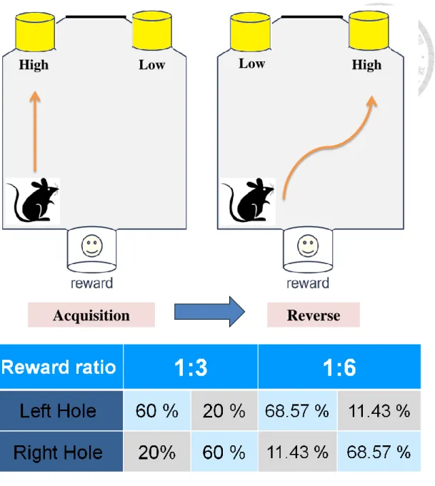
& Glimcher, 2009). It was a two-alternative forced-choice task, and one of the alternative apertures presented a reward at a high rate, while independently, the probability of receiving a reward in the other aperture was low. Animals conducted a 45-min daily session per day. The procedure consisted of a shaping phase and a 2-reward-ratio testing phases: the 1:3 reward ratio and the 1:6 reward ratio, as depicted in Figure 2. 2.
3.5.1. Shaping phase. Before surgery, mice were first trained to operate the
experimental apparatus by a series of 4 shaping stages. In each stage, each mouse was required to reach shaping criteria in 45 minutes, and then they could move to the next stage. During the first 4 shaping stages, a trial started with the illumination of the house light, and ended after animals collected their reward following a new trial started automatically. Besides, the magazine illuminated to signal the delivery of a reward. Stage 1 (MAG10): Animals were required accumulating 10 nose pokes into either the 2 stimulus-response apertures or the magazine, and each nose poke was followed by the delivery of a reward. Stage 2 (M5H5): Animals were still required to perform a nose poke into the magazine followed by the delivery of a reward. But after
28
accumulating 5 nose pokes into the magazine, no reward was delivered from the magazine if the animal kept performing nose pokes into the magazine. Each mouse was required accumulating 5 nose pokes into one of the 2 apertures, and each nose poke into stimulus-response apertures was followed by the delivery of a reward. Stage 3 (M0H10): Each mouse was required accumulating 10 nose pokes into one of the 2 stimulus-response apertures, and nose poking into the magazine was not followed by any delivery of a reward. Additionally, each nose poke into stimulus-response
apertures was followed by the delivery of a reward. Stage 4 (H11): A trial started with the illumination of the house light, and then mice had to wait an intertrial interval (ITI) of 5 sec for the illumination of stimulus-response apertures. The 2 apertures
subsequently illuminated, and animals were required to accumulating 11 nose pokes into one of the illuminated apertures to show their preference for left or right
stimulus-response apertures, and each nose poke into apertures was followed by the delivery of a reward.
3.5.2. Testing phase. After surgery, mice went on shaping phase (only stage 4)
again to show their preference for left or right stimulus-response apertures. After mice completed stage 4, next day started the testing phase. The testing phase consisted of 2 reward ratio testing phases: the 1:3 reward ratio (including acquisition of the 1:3
29
reward ratio and reversal of the 1:3 reward ratio); the 1:6 reward ratio (including acquisition of the 1:6 reward ratio and reversal of the 1:6 reward ratio). The 1:3 reward ratio contained the reward rate of 20 % and 60 % in one of the 2
stimulus-response apertures. The 1:6 reward ratio had the reward rate of 11.43% and 68.57% in one of the 2 stimulus-response apertures. The location of high and low reward aperture was switched back and forth one day after each mouse completed preset criteria in each section, as shown in Figure 2. 2. On each day, each animal underwent a 45 minutes daily session or maximum 6 blocks (a block consisted of 10 trials). Daily session began with the illumination of house and magazine lights. A nose poke into the magazine initiated a trial and extinguished the magazine light. A fixed ITI of 5 sec preceded the illumination of stimulus-response apertures. The 2
stimulus-response apertures subsequently illuminated after the ITI, and animals were required nose poking into one of the illuminated apertures. Each nose poke into the illuminated aperture was followed by either the delivery of a reward or no any reward, and both of them were subsequently followed by the illumination of magazine. Each trial ended after animals collected earned reward or after animals nose poked into the illuminated magazine. Each mouse discovered these rules and chose the high reward rate aperture by trial and error. The criteria of accomplishing each section was
30
accumulating choice of the high reward rate aperture for at least 70% accuracy in 3 consecutive blocks. Once the criterion was achieved, each mouse moved on to the next section on the next testing days and the reward rates of the 2 apertures were switched. If mice couldn’t reach the criterion after accumulating over 900 trials, mice also moved on to the next section on the next testing days. Accumulated trials, choice results, and latency both to response to the illuminated apertures and to reach the magazine were recorded trial by trial by computer software during daily training.
3.6. Histology. Mice were perfused and the brains post-fixed with 4%
paraformaldehyde, with lesion placement identified through Nissl staining of 40-μm brain slices. Only mice with lesions located with DMS, DLS or OFC were included.
4. Data analysis
4.1. Q learning model. A standard reinforcement learning model was applied to
estimate RPE in the 2-choice dynamic foraging task. As typically seen in other modeling work, the reinforcement learning model constitutes one value updating component (i.e. how information is updated) and one choice component (i.e. how choice is made). For the value updating rule, we used a simplified Q-learning model, which belongs to the family of temporal difference models, to characterize the
dynamic process of RPE in the 2-choice dynamic foraging task (Sutton & Barto, 1998;
31
Watkins & Dayan, 1992). Such a rule proposes that an RPE is updated whenever the subject’s expected reward changes on each trial. Thus, the value chosen from the
high-reward aperture for each trial was updated according to the following rule (Rutledge et al., 2009).
α where Qhigh(t) is the expected value associated with choosing the high-reward rate aperture on trial t and (t) is the RPE representing the discrepancy between expectation and the reward just received. Rhigh(t) denotes the actual outcome received from the high-reward rate aperture on trial t. The parameter α represents the learning rate, which determines how rapidly the reward prediction error signal is updated.
Because the onsets of stimuli and outcomes were modeled trial-by-trial as separate (t)
at the time of each feedback display during each trial, the magnitude of RPE was determined by the learning rate (α) from the trial-by-trial data in each testing section
of the 2-choice dynamic foraging task.
Reinforcement learning also requires a balance between exploration and exploitation. For the choice rule in the reinforcement learning model, it is assumed that the probability of choosing the high-reward aperture Phigh(t + 1) was determined
32
by the so-called softmax rule or Boltzmann exploration (Kaelbling et al., 1996), a logistic form that assigned a weight to each of the actions according to their action value estimation:
The parameter β represents choice perseveration (or exploration/exploitation), a
term referring to the tendency of making actions guided by reward values. A zero value of β means the subject will choose the high-reward rate aperture at random. To estimate the learning rate (α) and the choice perseveration (β), we used a hierarchical
modeling approach called Markov Chain Monte Carlo (MCMC)-based Bayesian parameter estimation to fit the reinforcement learning model to the trial-by-trial data from the 2-choice dynamic foraging task (Lee & Wagenmakers, 2014; Wetzels, Lee,
& Wagenmakers, 2010). The advantage of the Bayesian approach is that it can account for inter-subject variability and other random effects in a more rigorous and satisfactory way using latent parameters. In particular, from the Bayesian perspective, parameters are described by informative probability distributions instead of point
33
estimations. A probit transformation was used to make the construction of the
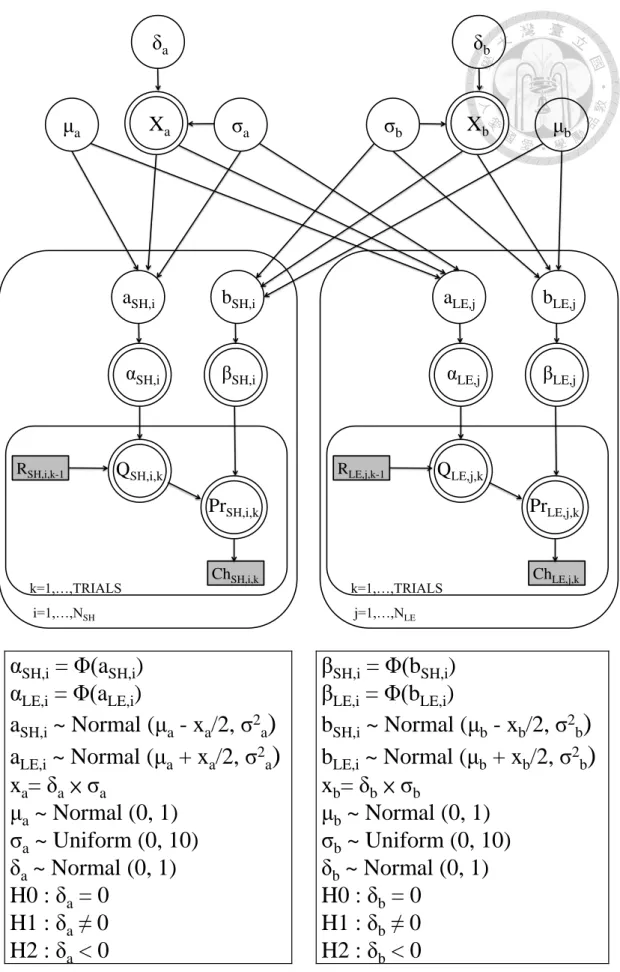
Bayesian hierarchical model easier. Because the Bayesian hierarchical model requires the number of input trials to be the same, we cut the cumulated trials into the same number by use of the smallest cumulated trials as a cutting point in the lesion and sham groups. The structure of this Bayesian hierarchical modeling is depicted in Figure 2. 3. As shown in Figure 2.3, the parameters α and β for subject i (αi and βi ) were each assumed normally distributed with respective means and standard deviations, which were from the group level of distributions (i.e. μa σa and μb σb , respectively). We used WinBUGS [the MS Windows operating system version of BUGS (Bayesian inference Using Gibbs Sampling)] and WinBUGS Development Interface (Lunn, Thomas, Best, & Spiegelhalter, 2000) to approximate the
distributions of parameters by sampling values using the MCMC technique. A chain consisted of 28000 iterations, of which the first 8000 (burn-in) points were discarded to ensure that only samples from the stationary distribution were used and that the data were unaffected by the starting value. Thus, we obtained 60000 points of estimation from the three chains and collected samples at intervals of every five samples, which yielded 12000 points. All interpretations and tests were performed based on these 12000 samples. Parameters between lesion and sham groups were
34
compared by computing the difference between the values of the two posterior
distributions in each run obtained from the hierarchical Bayesian estimation. One way to evaluate the strength of evidence for differences in group-mean parameters is by checking whether the probability of the posterior distribution of differences is greater (or less) than zero (Fridberg et al., 2010). Another way is to use the Bayes factor (BF), an odd ratio of marginal likelihood of the two models (or hypotheses) of interest, to index the evidence strength of the alternative hypothesis against the null hypothesis
(Kass & Raftery, 1995; Raftery, 1995). A large BF value ( > 3) would (at least)
“positively” favor the alternative hypothesis and a BF value between 1 and 3 would
“weakly” favor the alternative hypothesis, as shown in Table 2. 1. To evaluate the
differences of group-mean parameters, a method based on the Savage-Dickey density ratio was used to compute the BF values (Wagenmakers, Lodewyckx, Kuriyal, &
Grasman, 2010).
35
4.2. Matching law analysis. To assess the degree to which animals in the
2-choice dynamic foraging task made their overall average choices in accord with the received rewards, a matching law analysis was also conducted (Baum, 1974; Rutledge et al., 2009), which provides a simple empirical quantification between the rate of
response and the rate of reinforcement:
In the above formula, Cleft and Cright denote the number of choices to the left- and right apertures, respectively. Likewise, Rleft and Rright are the respective number of rewards received from the left and right apertures. The slope s is thought to be a measure of the sensitivity of choice allocation to reward frequency. In this study, we used least-squares regression to fit the above formula to steady-state (last 30 trials of each testing phase) choice behavior in the 2-choice dynamic foraging task. Blocks in which one aperture was never rewarded (i.e. R left or Rright = 0) were excluded from the analysis in order to fit the data to the above formula.
4.3. Statistical analysis and software. The behavioral data were analyzed by
the Student’s t-test or the one-way analysis of variance (ANOVA) where appropriate.
Adjusted t-test was applied if the Levene’s test for equality of variances reached the
36
significant level. Statistic analyses were performed using SPSS 20.0 (SPSS Inc., Chicago, IL, USA).
37
Chapter 3: Results
1. Histology
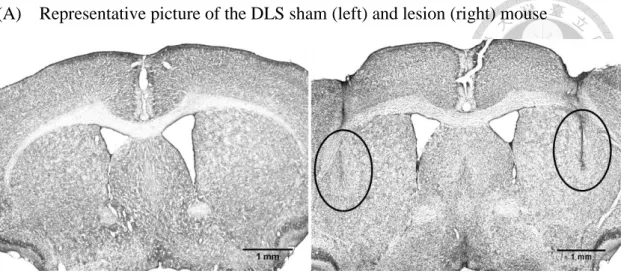
Photographs of representative infusion placements in the DLS, DMS and NA were shown in Figure 3. 1. Using Nissl staining, 3 of 13 mice in the DLS lesioned group were excluded from the study; 5 of 15 mice in the DMS lesioned group were excluded from the study; 5 of 15 mice in the NA lesioned group were excluded from the study, as shown in Figure 3. 2.
2. Behavioral data
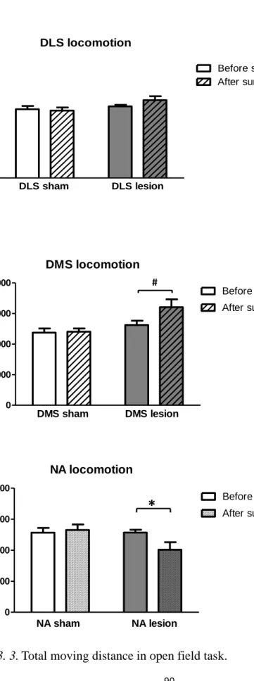
2.1. Open field task. As shown in Figure 3. 3, no significant difference was found
in the three sham groups before surgery (F(2,27) = 0.817, p = .452) and after surgery (F(2,27) = 1.933, p = .164). No significant difference was found in the DLS lesioned mice after surgery (t(9) = -1.324, p = .22). A trend of hyperlocomotion was found in the DMS lesioned mice after surgery (t(9) = -2.184, p = .057). The NA lesioned mice showed hypolocomotion after surgery (t(9) = 2.602, p = .029 ).
2.2. Sucrose preference test. As depicted in Figure 3. 4, no significant difference
was found in the three sham groups in sucrose preference (F(2,27) = 1.115, p = .343) There is no significant difference in sucrose preference between lesioned mice and
38
sham controls within each of the 3 groups (DLS: t(18) = 0.169, p = .87; DMS: t(18) = -1.607, p = .13; NA: t(18) = -0.797, p = .44).
2.3. Assessing motivation on performing the 2-choice task after surgery. In
these 3 brain lesioned groups, there is no difference in latency to response to the illuminated apertures before and after surgery (DLS: t(9) = 0.266, p = .80; DMS: t(9)
= 0.146, p = .89; NA: t(9) = 0.034, p = .97), as shown in Figure 3. 5. There is no difference in latency to collect reward between lesioned mice and sham controls within each of the 3 groups (DLS: t(9) = -0.908, p = .39; DMS: t(9) = -0.148, p = .89;
NA: t(9) = -0.412, p = .69), as shown in Figure 3. 6. No significant difference was found in the three sham groups in latency to response to the illuminated apertures before (F(2,27) = 0.096, p = .909) and after surgery (F(2,27) = 0.881, p = .426). No significant difference was found in the three sham groups in latency to collect reward before (F(2,27) = 0.250, p = .781) and after surgery (F(2,27) = 0.508, p = .607).
2.4. Measurement of cumulated trials and errors in the 2-choice dynamic
foraging task. For overall cumulated trials, no significant difference was found in the
three sham groups (F(2,27) = 0.144, p = .866). For overall cumulated trials, no significant difference was found in the DLS (t(18) = -0.791, p = .44) and NA (t(18) = -1.479, p = .16) groups. Compared to sham mice, the DMS lesioned mice required
39
more overall trials to reach the preset criteria (t(10.547) = -2.576, p = .027), as shown in Figure 3. 7. For cumulated trials in the 1:3 reward ratio and the 1:6 reward ratio, no significant difference was found in the three sham groups (1:3 reward ratio: F(2,27) = 0.472, p = .629; 1:6 reward ratio: F(2,27) = 0.211, p = .811). For cumulated trials in the 1:3 reward ratio and the 1:6 reward ratio, no significant difference was found in the DLS group (the 1:3 reward ratio, t(18) = -0.406, p = .69; the 1:6 reward ratio, t(18)
= -1.274, p = .22). Compared to sham mice, the DMS lesioned mice required more cumulated trials to reach the preset criteria in the 1:6 reward ratio (t(18) = -2.155, p
= .045) and there is a marginal significant difference in the 1:3 reward ratio (t(11.976)
= -2.089, p = .059). Compared to sham controls, a trend in the 1:3 reward ratio was found in the NA lesioned mice (t(13.487) = -2.049, p = .06), as shown in Figure 3. 8.
For cumulated trials in the learning of 1:3 reward ratio, the reversal of 1:3 reward ratio, learning of 1:6 reward ratio, and reversal of 1:6 reward ratio, no significant difference was found in the DLS (1: t(18) = -1.668, p = .11; 2: t(18) = 0.441, p = .67;
3: t(11.536) = -1.168, p = .27; 4: t(18) = -1.119, p = .28) and DMS (1: t(10.316) = -1.278, p = .23; 2: t(12.971) = -1.122, p = .28; 3: t(18) = -1.719, p = .10; 4: t(18) = -1.341, p = .20) groups. For cumulated trials in every section, no significant difference was found in the three sham groups (1: F(2,27) = 0.693, p = .509; 2: F(2,27) = 2.182,
40
p = .132; 3: F(2,27) = 0.641, p = .535; 4: F(2,27) = 0.012, p = .988). But as shown in
Figure 3. 9, compared to sham controls, a trend on cumulated trials was found in the NA lesioned mice (t(9.933) = -2.035, p = .069)in the reversal of the 1:3 reward ratio.
For overall cumulated errors, no significant difference was found in the three sham groups (F(2,27) = 0.031, p = .969). For overall cumulated errors, no significant difference was found in the DLS (t(18) = -0.975, p = .34) and NA (t(18) = -1.396, p
= .18) group. Compared to sham mice, the DMS lesioned mice cumulated more total errors to reach the preset criteria (t(9.885) = -2.583, p = .028), as shown in Figure 3.
10. For cumulated errors in the 1:3 reward ratio and the 1:6 reward ratio, no
significant difference was found in the three sham groups (1:3 reward ratio: F(2,27) = 0.661, p = .525; 1:6 reward ratio: F(2,27) = 0.945, p = .401). For cumulated errors in the 1:3 reward ratio and the 1:6 reward ratio, no significant difference was found in the DLS group (the 1:3 reward ratio, t(18) = -0.594, p = .56; the 1:6 reward ratio, t(18)
= -1.546, p = .14). Compared to sham mice, the DMS lesioned mice cumulated more errors to reach the preset criteria in the 1:6 reward ratio (t(18) = -2.223, p = .039) and there was a marginal difference in the 1:3 reward ratio (t(10.487) = -2.110, p = .06).
There is a trend that the NA lesioned mice cumulated more errors to reach the preset criteria in the 1:3 reward ratio compared to sham mice (t(11.953) = -1.869, p = .086),
41
as shown in Figure 3. 11. For cumulated errors in each of the four sections, no significant difference was found in the DLS (1: t(18) = -1.397, p = .18; 2: t(18) = -0.036, p = .97; 3: t(18) = -1.219, p = .24; 4: t(18) = -1.291, p = .21) and DMS (1: t(18)
= -1.337, p = .20; 2: t(18) = -1.216, p = .24; 3: t(18) = -1.723, p = .10; 4: t(18) = -1.027, p = .32) groups; whereas the NA lesioned mice seemed to cumulate more errors in the reversal of 1:3 reward ratio compared to sham mice (t(9.983) = -1.974, p
= .077), as shown in Figure 3. 12. For cumulated errorss in every section, no significant difference was found in the three sham groups (1: F(2,27) = 1.119, p
= .341; 2: F(2,27) = 2.076, p = .145; 3: F(2,27) = 1.711, p = .200; 4: F(2,27) = 0.110, p = .897).
3. Matching law analysis
Using least-squares regression, trial-by-trial data from the steady state (last 30 trials in each section) of the 2-choice dynamic foraging task were fitted and used to estimate reward sensitivity. The sections in which animals gained no reward from either of the two apertures (i.e., R low or Rhigh = 0) were excluded from analysis. As depicted in Figure 3. 13, the estimated values of reward sensitivity s for the DLS sham and lesion groups were 0.607 and 0.616, respectively. The estimated values of reward
42
sensitivity for the DMS sham and lesion groups were 0.60 and 0.569, respectively.
And the estimated values of reward sensitivity for the DLS sham and lesion groups were 0.676 and 0.611, respectively. There is no significant difference in reward sensitivity between sham controls and lesioned mice within each of the three groups (DLS: t(56) = 0.247, p = .81; DMS: t(47) = -0.546, p = .59; NA: t(51) = 0.536, p
= .60).
4. Estimation of learning rate and choice perseveration using reinforcement
learning model
As depicted in Figure 3. 14, the posterior sample means and their 95% credible intervals (CI) of learning rate (α) for the DLS sham and lesion groups were 0.0072 (CI
= (0.0040, 0.0124)) and 0.0069 (CI = (0.0036, 0.0120)), respectively. The posterior sample means and their 95% credible intervals (CI) of learning rate (α) for the DMS sham and lesion groups were 0.0074 (CI = (0.0038, 0.0137)) and 0.0033 (CI = (0.0014, 0.0068)), respectively. The posterior sample means and their 95% credible intervals (CI) of learning rate (α) for the NA sham and lesion groups were 0.0078 (CI
= (0.0048, 0.0124)) and 0.0039 (CI = (0.0023, 0.0065)), respectively. Besides, the probability of the posterior distribution of group mean differences of the parameter α
43
between sham and lesion groups for the DLS, DMS and NA groups were 0.556, 0.957, and 0.978, respectively. The Results from the DMS and NA groups provided marginal evidence in favor of the claim that the learning rate of sham group was higher than lesion group. The findings in DMS and NA groups are further supported by the Bayesian hypothesis test, in which we obtained BF = 3.15 and 7.10, respectively. The BF values are positively in favor of the evidence that the learning rate in the lesion (DMS and NA) groups are lower than their corresponding sham groups.
As depicted in Figure 3. 15, the posterior sample means and their 95% credible intervals (CI) of choice perseveration (β) for the DLS sham and lesion groups were 2.92 (CI = (1.89, 4.26)) and 2.77 (CI = (1.81, 4.02)), respectively. The posterior sample means and their 95% credible intervals (CI) of choice perseveration (β) for the DMS sham and lesion groups were 3.67 (CI = (1.52, 6.55)) and 5.98 (CI = (2.90, 8.86)), respectively. The posterior sample means and their 95% credible intervals (CI) of choice perseveration (β) for the NA sham and lesion groups were 3.55 (CI = (1.28, 6.51)) and 6.21 (CI = (3.19, 8.92)), respectively. Besides, the probability of the posterior distribution of group mean differences of the parameter β between lesion and sham groups for the DLS, DMS and NA groups were 0.424, 0.876, and 0.902, respectively. The findings in DMS and NA groups are further supported by the