含缺陷與界面之平板邊界元素分析

國 立 成 功 大 學

航 空 太 空 工 程 學 系 博 士 論 文

含缺陷與界面之平板邊界元素分析

Boundary Element Analysis for Plates with Defects and Interfaces

研 究 生：陳昱志 Student : Yu-Chih Chen 指導教授：胡潛濱 Advisor : Chyanbin Hwu

Department of Aeronautics and Astronautics National Cheng Kung University

Tainan, Taiwan, R.O.C.

Dissertation for Doctor of Philosophy

July 2013

國 立 成 功 大 學

航 空 太 空 工 程 學 系 博 士 論 文

含缺陷與界面之平板邊界元素分析

Boundary Element Analysis for Plates with Defects and Interfaces

研 究 生：陳昱志 Student : Yu-Chih Chen 指導教授：胡潛濱 Advisor : Chyanbin Hwu

Department of Aeronautics and Astronautics National Cheng Kung University

Tainan, Taiwan, R.O.C.

Dissertation for Doctor of Philosophy July 2013

中 華 民 國 一 ０ 二 年 七 月

Boundary Element Analysis for Plates with Defects and Interfaces

Yu-Chih Chen

A Dissertation Submitted to

the Faculty of the Department of Aeronautics and Astronautics National Cheng Kung University

in Partial Fulfillment of the Requirements for the Degree of

Doctor of Philosophy

本簽名業格式請參考航太系碩博士學生手冊

A4紙整頁掃瞄後以圖片方式插入，尺寸：100%，配置：文繞圖（矩形、置中），

圖片位置（水平對齊相對於頁/置中對齊，垂直對齊相對於頁/靠上）

簽名頁

摘要

論文題目(中文)：含缺陷與界面之平板邊界元素分析

論文題目(英文)：Boundary Element Analysis for Plates with Defects and

研 究 生：陳昱志 指導教授：胡潛濱

本研究重點在於將異向性彈性材料中已滿足特殊問題邊界條件之格 林函數，透過通用形式之邊界元素分析，將問題由異向性彈性材料延伸 至壓電與黏彈性材料，並拓展至動態分析。在廣大的工程研究領域中，

奇異性問題的求解與如何提高解的精確度，一直都是研究者深感興趣與 極具挑戰的議題。於機械力學，奇異性問題通常發生在幾何不連續或材 料不連續處，如同本論文關注的平板含缺陷(孔洞、裂縫與異質)與界面等 相關問題，雖然這些問題早已存在著解析解，但若遇到較複雜的幾何外 形與外力負載，還是需要藉助數值方法來求解問題。邊界元素法是數值 方法中處理此特殊問題(如板含孔洞、裂縫、異質、界面等)較有效且準確 的，其最大的特色在於可以減少求解問題的維度，且若使用的基本解滿 足問題的邊界條件，在邊界上之分析結果將會完全滿足。針對二維異向 性彈性材料，許多基本解如無限域含孔洞、裂縫、異質與界面等問題，

已透過史磋複變公式導出，相關邊界元素法之應用也已被證實可改善數 值分析的精確度並可節省電腦分析時間。

壓電材料之電彈耦合本構方程式可經由彈性材料方程式之維度擴充

而得，由於兩者具有相同的數學模型，故壓電材料的解可直接由相對應

之彈性材料的解擴充維度而得到。相同地，藉由彈性體與黏彈性體間之 對應法則，彈性材料的解也可應用於黏彈性材料的解，於拉普拉斯域中。

因此，透過上述的對應法則，彈性材料的基本解與邊界積分式，皆可應 用於壓電與黏彈性材料。此外，藉由邊界元素法中的雙互換定理，若將 動態問題的慣性力視為廣義的體力，則靜態問題的基本解也可用於求解 動態問題之邊界元素法中。

基於上述論點，為了展現孔洞/裂縫/異質/界面之格林函數成功地應用 於異向性彈性體、壓電體與黏彈性體或動態問題中，許多數值分析案例，

如異向性彈性/壓電/黏彈性二維平板含孔洞/裂縫/異質/界面之靜態問題 與異向性彈性二維平板含孔洞/裂縫/界面之動態問題等，將於本論文中呈 現。

關鍵字：異向性彈性材料、格林函數、邊界元素分析、壓電材料、黏彈 性材料、奇異性、孔洞、裂縫、異質、界面、史磋複變公式、

雙互換定理。

Boundary Element Analysis for Plates with Defects and Interfaces

Student: Yu-Chih Chen Advisor: Chyanbin Hwu

ABSTRACT

The problems concerning with singularity and how to obtain accurate results from

them are the topics which greatly interest and challenge to the researchers all the while. In

solid mechanics, such singularities are resulted from discontinuities of geometry or

material heterogeneity, such as a plate with defects (holes, cracks, inclusions) and

interfaces. Although a lot of exact solutions for those critical problems have been derived

mathematically, the numerical analyses are still needed for some problems which involve

the complex geometry and loading conditions. That is why we endeavor to solve such

problems engaged with the boundary element method (BEM). The main advantages of

BEM are the reduction of the dimension of the problem by one and the exact satisfaction of

certain boundary conditions in some particular problems if their associated fundamental

solutions are embedded in boundary element formulation. Because the fundamental

solutions satisfy the boundary conditions of the defects and interface, say, no meshes are

needed along the boundaries of holes, cracks, inclusions or interfaces in BEM. For

two-dimensional anisotropic elasticity, many fundamental solutions, the so called Green’s

functions of BEM, have been derived by using the complex variable Stroh formalism, such

as an infinite space with holes, cracks, inclusions and interfaces, etc. Several researches in

this field have proved that by using such fundamental solutions for BEM it makes the task

more efficient and the results more accurate when coping with these problems.

Since the mathematical formulation of piezoelectric elasticity can be organized into the same form as that of anisotropic elasticity by just expanding the dimension of the corresponding matrix to include the piezoelectric effects, the solutions to the problems of piezoelectric materials can be obtained immediately through the extension of the solutions to the associated anisotropic elastic materials. Similarly, with the aid of the correspondence between elastic and viscoelastic materials, solutions for the linear anisotropic elastic solids can be applied directly to the linear anisotropic viscoelastic solids in the Laplace domain.

With this understanding, one can acquire the fundamental solutions and boundary integral equations for piezoelectric and viscoelastic problems. Moreover, by using the dual reciprocal theorem for BEM, the static fundamental solutions can be used for dynamic boundary element method if the inertia term of the latter is treated as a general body force, which is the source term remained in the domain integral.

Based on the discussion above, in addition to the dynamic analysis of two-dimensional plates containing holes, cracks, and interfaces, several examples are also demonstrated in this dissertation to show that the static fundamental solutions of holes, cracks, inclusions and interfaces in anisotropic elasticity, derived in the sense of Stroh formalism, and the associated boundary integral equations have been extended to the applications for the piezoelectric and viscoelastic problems successfully with the prominence of accuracy and efficiency of the present BEM.

Key words: Singularity, Holes, Cracks, Inclusions, Interfaces, Boundary Element Method,

Anisotropic Elasticity, Green’s Function, Stroh Formalism, Piezoelectricity,

Viscoelasticity, Dual Reciprocal Theorem.

第一章 緒論

有限元素法與邊界元素法是目前廣泛應用於應力數值分析的工具之 二，雖然有限元素法較為大眾接受，但針對一些特殊的問題，如板含孔 洞、裂縫、異質及界面等，若邊界元素法之基本解已滿足特定之邊界條 件，則會比有限元素法來的準確及有效率，且分析時無須對孔洞、裂縫、

異質或界面等邊界進行元素切割，如此一來可節省前處理過程與程式求 解時間。針對異向性彈性材料，上述特殊問題之解析解及邊界元素法的 應用已有相關文獻產出，也證實使用滿足邊界條件基本解之邊界元素法，

其準確性與效率性較優於傳統邊界元素法或有限元素法，因此，如何將 此特殊邊界元素法之優越性延伸至壓電材料、黏彈性材料，甚至拓展至 動態問題，為本論文的主要目的。

藉由觀察異向性彈性體與壓電體、黏彈性體間基本方程式的差異，

可從中找出相互間的對應關係，藉由此對應關係可將異向性彈性體的通 解延伸至壓電體與黏彈性體。本論文中，邊界元素分析之基本解採用滿 足特定問題(如孔洞、裂縫、異質、界面)邊界條件之格林函數，是透過 史磋複變形式公式所推導而得，因史磋公式有著優美且簡約的數學模型，

加上上述材料模型之對應關係，使得基本解於異向性彈性、壓電性、黏 彈性材料間具有同樣的張量表示式。同樣的透過對應法則，對於求解異 向性彈性、壓電與黏彈問題之邊界積分式，也具有相同的表示式。此外，

針對動態問題，若是邊界元素分析之基本解是採用靜態問題之格林函數，

會導致與時間相關的慣性力或體力保留在體積分中，在此藉助雙互補定

律將體積分轉換至邊界積分，使邊界元素法依然保有僅處理邊界積分之

特性。最後，結合上述理論架構，本論文提出一通用形式之靜態/動態邊

界元素分析，可處理異向性彈性/壓電性/黏彈性平板含缺陷與界面等問

題，透過數值案例與現存之解析解或其它數值結果比較，呈現本論文使

用特殊格林函數之邊界元素所具有之精確性及效率性。

第二章 史磋公式

處理二維異向性彈性材料的方法中，史磋公式是常用的解法之一，

其特色為使用複變函數進行解題，倚賴位移的協和方程式，搭配應變-位 移關係式、材料組成率與力平衡方程式發展而成。史磋公式理論採用之 通解形式與相關物理量之表示式，會呈現在本章節中。另外，經由基本 方程式的觀察，可發現異向性彈性材料與壓電材料及黏彈性材料間的對 應關係，因此，若欲得到壓電材料與黏彈性材料的通解，不需要再重新 推導，只需透過彼此之間的對應關係於彈性解中求得即可。簡單來說，

壓電材料的通解可經由彈性材料的解將其矩陣維度擴增，而使其具有電

彈耦合之特性；黏彈性材料的通解可透過彈性材料的解建構於拉普拉斯

域中，欲得時間域的解只需要將其做拉普拉斯逆運算即可。

第三章 邊界元素分析

邊界元素分析所使用的基本解，是點荷重作用於無限域下控制微分 方程式的解析解，其精確解也使得邊界元素分析較有限元素分析準確，

特別是針對應力集中或牽涉無限域或半無限域之問題。邊界元素法是將 邊界積分式以離散化方式建構而成的數值方法，如同前章節所述，處理 彈性材料之邊界積分式，可經由一些對應關係拓展至壓電及黏彈性材料。

另外，透過雙互換原理，對於動態邊界元素分析之基本解亦可採用靜態

格林函數。本章將介紹靜態邊界元素分析於彈性體、壓電體與黏彈性體

的理論架構，並說明如何運用雙互換定理處理動態問題。

第四章 基本解與特殊解

針對孔洞/裂縫/異質/界面等問題，利用史磋公式推導滿足特殊邊界

條件之格林函數，將其運用於邊界元素分析之基本解中，如此可省略內

部特殊邊界之元素切割，只需對外部邊界做切割即可，許多異向性彈性

材料之解析解可於文獻中(Ting, 1996與Hwu, 2010)得到，在此只呈現異向

性彈性材料含孔洞/裂縫/異質/界面等問題之基本解，針對壓電材料與黏

彈性材料則是透過第二章所述之對應關係中求得。對於動態問題，運用

雙互換定理所需要的特殊解也在此做一介紹。

第五章 數值範例

為了展示前幾章理論基礎之成果，此章將執行多個數值範例分析，

包含異向性彈性/壓電/黏彈性二維平板含孔洞/裂縫/異質/界面之靜力

問題，與異向性彈性二維平板含洞/裂縫/界面之自由振動與強迫振動分

析，數值結果會與現有之理論解或其他數值方法進行分析比較，以驗證

本論文所提出之邊界元素法之優越性與準確性。

第六章 結論

本論文中透過彈性體/壓電體、彈性體/黏彈性體間的相互關係，與 邊界元素法之雙互換定律，成功的將異向性彈性孔洞/裂縫/異質/界面之 基本解運用於異向性壓電/黏彈性材料，及求解動態邊界元素分析上，因 基本解滿足特殊問題之邊界條件，故執行邊界元素分析時，只需針對外 部邊界做切割，此特性可使分析結果更為準確，並且節省數值分析的時 程，也因內部邊界無須做元素切割，對於求解靠近孔洞/裂縫/異質/界面 之點位應力值時，會有較穩定之數值表現，透過一系列的數值分析顯示，

含孔洞/裂縫/異質等靜態問題，採用8個元素即可得到精確之全域解，即 使用靠近裂縫尖端的應力場計算應力強度因子，也可得到相當收斂之結 果，針對含界面之靜態問題，至多16個元素也可得到令人滿意之精度。

至於動態問題，因為模態分析的需要，若要在高頻部分有精確的分析結

果，則需要較多元素來描述高頻的變形行為，大致24~48個元素即有不錯

的表現。最後，數值結果證明本論文所提及之邊界元素法具有相當之優

越性與準確性。

誌謝

首先誠摯的感謝指導教授胡潛濱博士，在學生修業期間總不厭其煩 的悉心教導並指引正確的方向，使學生得以一窺異向性固體力學的奧秘 並獲益匪淺。另外，也感謝碩士班指導教授黃立政博士，當初若不是黃 老師的鼓勵與建言，學生也不會有萌生博士求學之路的想法。如今求學 生涯即將劃上句點，當初的堅持，終有成果，在感到欣慰之餘，期許自 己未來也能夠持續秉持著這股熱忱的態度，不斷地努力及突破。

本論文的完成，除了感謝胡潛濱教授細心指導外，還要感謝瀚文學 弟在英文方面的指正，漫長的求學生涯中，很開心能夠認識5912師門的 學長姐、學弟妹與同儕們，一同上山下海熬夜拼寫作業、分享歡樂與悲 傷；特別要感謝豪義、育魁、瀚文及仲喬在求學階段給予我行政庶務上 的協助，尤其是在博士班口試階段，還好有大家的鼎力相助，才不致於 讓我分身乏術，在此由衷地感謝大家。

最後，謹以此文獻給我摯愛的雙親與親朋好友。

僅誌於

國立成功大學 航空太空工程學系博士班

中華民國一０二年七月

CONTENTS

摘要 ... i

ABSTRACT ... iii

誌謝 ... xii

CONTENTS ... xiii

LIST OF TABLES ... xv

LIST OF FIGURES ... xvi

NOMENCLATURE ... xix

CHAPTER Ⅰ INTRODUCTION ... 1

CHAPTER Ⅱ STROH FORMALISM ... 6

2.1 Anisotropic Elasticity ... 6

2.2 Piezoelectric Materials ... 9

2.3 Viscoelastic Materials ... 11

CHAPTER Ⅲ BOUNDARY ELEMENT ANALYSIS ... 16

3.1 Static Analysis ... 16

3.1.1 Boundary Integral Equations for Statics ... 16

3.1.2 Boundary Element Formulation for Statics ... 18

3.1.3 Subregion technique ... 20

3.1.4 Anisotropic Elastic Materials ... 21

3.1.5 Piezoelectric Materials ... 21

3.1.6 Viscoelastic Materials ... 21

3.2 Dynamic Analysis ... 23

3.2.1 Boundary Integral Equations for Dynamics ... 23

3.2.2 Boundary Element Formulation for Dynamics ... 25

3.2.3 Free Vibration ... 26

3.2.4 Forced Vibration ... 27

3.2.5 Transient Analysis ... 28

3.2.5.1 Houbolt’s algorithm ... 28

3.2.5.2 Modal superposition method ... 30

4.1 Fundamental Solutions ... 33

4.1.1 Holes or Cracks ... 36

4.1.2 Inclusions ... 36

4.1.3 Interfaces ... 37

4.2 Particular Solutions ... 38

CHAPTER V NUMERICAL EXAMPLES ... 40

5.1 Anisotropic Elastic Plates ... 40

5.2 Piezoelectric Plates ... 44

5.3 Viscoelastic Plates ... 47

5.4 Dynamic Problems ... 57

CHAPTER VI CONCLUSIONS ... 65

REFERENCES ... 67

PUBLICATION LIST ... 126

LIST OF TABLES

Page Table 5.1 : The strains and stresses at interfacial point A obtained from BEM and

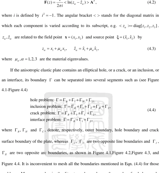
exact solutions. ... 73 Table 5.2 : Material constants of PZT-4, PZT-5H, PZT-7A and p-elastic. ... 74 Table 5.3 : Natural frequencies of an anisotropic elastic plate with an elliptical hole. 75 Table 5.4 : Natural frequencies of an isotropic plate with crack in different crack

lengths (L=6 m, a=0~2 m,  =0

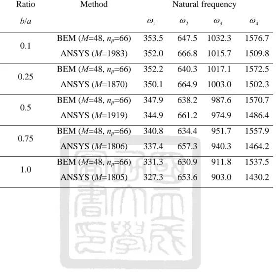
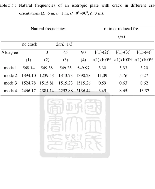
,  =3m). ... 76 Table 5.5 : Natural frequencies of an isotropic plate with crack in different crack

orientations (L=6 m, a=1 m,  =0

~90

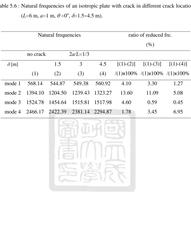
,  =3m). ... 77 Table 5.6 : Natural frequencies of an isotropic plate with crack in different crack

locations (L=6 m, a=1 m,  =0

,  =1.5~4.5m)... 78

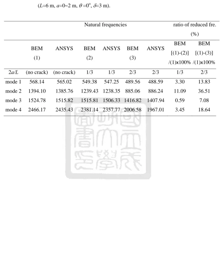
Table 5.7 : Natural frequencies of an anisotropic elastic plate with a crack. ... 79

LIST OF FIGURES

Page

Figure 4.1  : The contour of integration for a plate with a hole. ... 80 

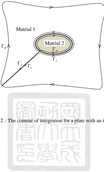
Figure 4.2  : The contour of integration for a plate with an inclusion. ... 81 

Figure 4.3  : The contour of integration for a plate with a crack. ... 82 

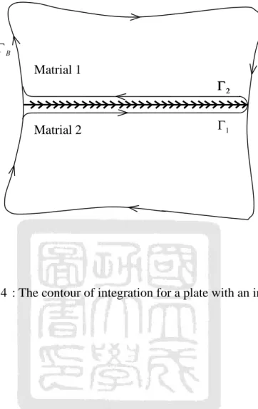
Figure 4.4  : The contour of integration for a plate with an interface. ... 83 

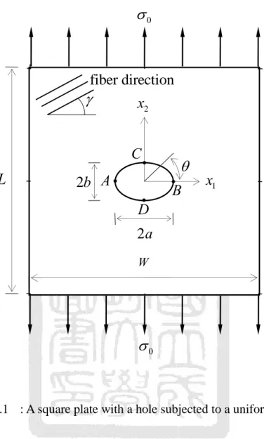
Figure 5.1  : A square plate with a hole subjected to a uniform loading. ... 84 

Figure 5.2  : Stresses along the hole in polar coordinate system. ... 85 

Figure 5.3  : A plate with a crack subjected to a uniform load... 86 

Figure 5.4  : The values calculated by Eqn.(5.4). ... 87 

Figure 5.5  : The hoop stresses of matrix calculated by BEM and ANSYS versus the value k. ... 88 

Figure 5.6  : (a) An infinite bi-material strip subjected to a uniform loading; (b) The geometry and boundary conditions of infinite bi-material strip set for BEM. ... 89 

Figure 5.7  : The stresses 

and 

along the interface calculated by BEM and ANSYS. ... 90 

Figure 5.8  : The crack opening displacement and relative electric potential caused by (a) a far-field stress 

 1 N/m

and (b) far-field electric displacement 1 C/m

 . ... 91 

Figure 5.9  : The electric displacement D

along the interface calculated by present BEM and ANSYS. ... 92 

Figure 5.10  :The (a) electric potential  and (b) electric displacement D

along the line x

=0 versus the value k defined in Table 5.2. ... 93 

Figure 5.11  : Comparison of the numerical Laplace inversion. ... 94 

Figure 5.12  : Time variations of the major and minor axes of the elliptical hole. ... 95 

Figure 5.13  : Crack opening displacements versus time and position. ... 96 

Figure 5.14  : Stress 

along the crack surface at t=0. ... 97 

Figure 5.15  : The mode I stress intensity factor K at t=0 calculated by the definition

(5.20) with small r. ... 98 

Figure 5.16  : A viscoelastic material with an elastic inclusion. ... 99 

Figure 5.17  : The stress  

/

at point A of Figure 5.16. ... 100 

Figure 5.18  : The hoop stress 

around the inclusion boundary (a)   0

; (b)   45

. ... 101 

Figure 5.19  : An interface corner between elastic and viscoelastic materials... ... 102 

Figure 5.20  : (a) Stresses 

at point (0.2, 0) versus time t ; (b) Stresses 

at

initial time versus location x along the interface. ... 103 

Figure 5.21  : A crack, hole and rigid inclusion in viscoelastic materials subjected to a uniform tension. ... 104  Figure 5.22  : Stress intensity factor K

versus distance (a) d and (b)

d for point A

and B. ... 105  Figure 5.23  : Multiple elastic fibers embedded in polymer matrix. ... 106  Figure 5.24  : Comparison of the effective Young’s modulus. ... 107  Figure 5.25  : (a) A square plate (a=6 m), and (b) a triangular plate (a=10 m, h=8 m)…..

... 108  Figure 5.26  : The interior source points of (a) a square plate and (b) a triangular

plate…. ... 109  Figure 5.27  : Natural frequencies for an isotropic square plate. ... 110  Figure 5.28  : Natural frequencies for an isotropic triangular plate. ... 111  Figure 5.29  : A rectangular plate subjected to a Heaviside-type load (   2 m ,

h  4 m ). ... 112  Figure 5.30  : Dynamic responses of (a) vertical displacement at point A and (b) normal traction at point B. ... 113  Figure 5.31  : A square plate with an elliptical hole subjected to a harmonic load

(   6 m, a  1 m, b  0.1 ~ 1 m ). ... 114  Figure 5.32  : Vibration mode shapes of an anisotropic elastic plate with a circular hole..

... 115  Figure 5.33  : Dynamic responses of vertical displacement at point C of the anisotropic elastic plate with a circular hole (M=24, n

=20 for BEM and M=1746 for ANSYS). ... 116  Figure 5.34  : Dynamic responses of stresses at point D calculated by (a) BEM (M=24, n

=20), and (b) ANSYS (M=1746) for the anisotropic elastic plate with a circular hole. ... 117  Figure 5.35  : A square plate with a crack subjected to a Heaviside-type load (   6 m )..

... 118  Figure 5.36  : Vibration mode shapes of an isotropic plate with a crack. ... 119  Figure 5.37  : (a) A geometry and (b) boundary element mesh and internal points of an orthotropic plate with a center crack subjected to a Heaviside-type load….

... 120  Figure 5.38  : Normalized dynamic stress intensity factor K K of the orthotropic

/

plate with a center crack. ... 121  Figure 5.39  : A bi-material square plate subjected to a Heaviside-type load





Figure 5.40  : Natural frequencies of a bi-material square plate (k=0.5~50). ... 123 

Figure 5.41  : Vibration mode shapes for a bi-material square plate (k=5). ... 124 

Figure 5.42  : Time variation of vertical displacement at point F of the bi-material plate

(k=5). ... 125 

NOMENCLATURE

b

body force

k

,

a b material eigenvectors

A B , material eigenvector matrices composed of a and

b

C

elastic stiffness tensor

E

Cijkl

elastic stiffness tensor at constant electric field

C

expanded elastic stiffness tensor for piezoelectric problem D

electric displacement

e

piezoelectric stress tensor E

electric field

( ) z

f an arbitrary function vector composed of f z which is assumed

(

) according to boundary and/or loading conditions

G shear modulus

E

electric field

I an identity matrix

, ,

I II III

K K K mode I, mode II and mode III stress intensity factors, respectively

N fundamental matrix

 mass density

Q R T , , material property matrix

s Laplace transform variable or the boundary curve S

elastic compliance tensor

t time

t

traction components

t traction vector composed of t

u

displacement components

u 

velocity

u

expanded displacement components for piezoelectric problem u (generalized) displacement vector

*

uij

,

fundamental solutions of displacement and traction

( )p

uij

,

particular solutions of displacement and traction ˆ

Ym

, G influence

coefficients

z

complex variable

ξ a vector composed of a

and b



strain components



expanded strain components for piezoelectric problem

 bulk modulus



material eigenvalues

 Poisson’s ratio

ik



dielectric permittivity tensor at constant strain



interpolation functions



natural frequencies

 (generalized) stress function vector



stress components



expanded stress components for piezoelectric problem

CHAPTER Ⅰ INTRODUCTION

In this dissertation the boundary element method (BEM) is employed for solving the problems with defects and interfaces. Such problems usually involve the singularity due to the geometric deformity or material discontinuity. The important features of BEM are reducing the dimension by one in solving problems and the competence of dealing with stress concentration or the problems which contain infinite or semi-infinite domains.

Mathematically, a crack in two-dimensional sense is a line with two coincide faces, which

leads to a degenerated geometry where no area exists but across which the displacement

field is discontinuous. Several special treatments have been devised to overcome this

difficulty, such as the displacement discontinuity method [1], the subregions method [2],

the dual boundary element method [3] and use of Green’s function for cracks [4]. In the

displacement discontinuity method, the differences of the displacement between the crack

surfaces are regarded as the unknown functions. The subregion method introduces the

notion of delimiting the artificial boundaries along the crack surfaces. As for the dual BEM,

the displacement boundary integral equation is applied on one of the crack surfaces and the

traction boundary integral equation on the other. All of the techniques above should have

the crack surfaces meshed except the one, the adequate use of Green’s function, which

dispense with the discretization along the cracks owing to the satisfaction of the

traction-free boundary condition. The limitation of this method is that it is only for the

problems with a traction-free crack. However, because of the use of the analytical solutions,

say, this type of Green’s function, the results of the BEM must be more accurate than the

others. Similarly, if the Green’s function for holes, inclusions and interfaces are utilized

analytically, the accuracy and efficiency of the BEM can be improved in the same manner as expected. For anisotropic elastic materials, the Green’s functions for hole, crack, inclusion and interface had already been derived analytically and the associated applications of BEM have been published in the literatures [5]-[12]. It can be proved that the BEM using these specific fundamental solutions is more accurate and efficient than conventional BEM or FEM. Hence, how to benefit from the predominance of these special BEM for anisotropic elasticity in other fields such as piezoelectricity, viscoelasticity, and the dynamic analysis employing those static fundamental solutions is the main purpose of this dissertation.

Through the correspondence between anisotropic elastic and piezoelectric materials

[12]-[16], the fundamental solutions for anisotropic elastic materials can easily be extended

to piezoelectric materials. Besides the boundary conditions in elastic field, those in electric

field are already satisfied the specific boundaries automatically if the associated solutions

in elastic problems are already satisfied the traction-free conditions of holes and cracks,

and continuity conditions of inclusions and interfaces. It is known that the solution forms

for anisotropic elastic materials and piezoelectric materials are exactly the same; the only

differences are the dimension and content of the matrices used in the solutions. Due to

these differences, when we consider the elastic/piezoelectric bi-material [17] or a

piezoelectric plate containing anisotropic elastic inclusions two different approaches are

considered. One is to re-derive the Green’s functions for these combinations, and the other

is to specialize the Green’s functions through general piezoelectric materials. For the

former one, we categorize the anisotropic elastic materials into two kinds, the conductors

and insulators. For the latter, the specialization is done by making the piezoelectric stress

tensor of anisotropic elastic materials zero, and letting the dielectric permittivity tensor be

zero or infinity to represent, respectively, the insulators or conductors.

In viscoelasticity, the materials exhibit a time rate of changes that is completely absent in the elastic materials. Due to the inclusion of time as an independent variable, the available exact analytical solutions have been obtained only for a few simplified problems.

Thus, to study the mechanical behavior of viscoelastic solids, the numerical approaches such as finite element method (FEM) and boundary element method (BEM) are usually needed. Generally, there are three different approaches for linear viscoelastic analysis by BEM. The first formulates a BEM in Laplace transform domain and is able to obtain the solution in time domain by numerical inversion [18][19]. The second formulates a BEM directly in time domain [20]-[22]. Although the second approach looks more direct and efficient, the lack of fundamental solutions in time domain has restricted its applicability.

To combine the advantages of the previous two approaches, a mixed BEM was proposed by Schanz [23], which can solve the problem in time domain but rely on the fundamental solutions in Laplace domain. Through the use of the correspondence mentioned above, the viscoelastic solids can be effectively treated in Laplace domain. To take the advantage of the available fundamental solutions for the defects or interfaces in anisotropic elastic materials [10]-[12], we choose the first approach, the transformed BEM, i.e., to treat the problems of viscoelastic solids containing defects such as holes, cracks or inclusions, or interfaces in this dissertation.

For the traditional BEM of dynamic analysis, the fundamental solutions used in the

boundary integral equation (BIE) are based on the solutions concerning the dynamic body

force, i.e., a unit impulse force, which is in terms of time variable. However, practically it

is difficult to find the solution analytically for particular problems, such as an anisotropic

elastic plate with cracks, holes, or interfaces subjected to an impulse force. Even though

such fundamental solutions could be obtained, the domain integral would be present in the

and Brebbia [25] developed the dual reciprocity boundary element method (DRBEM) to deal with the problems which involve the domain integral. By using a series of distributed shape functions to approximate the source term, the domain integral can be transformed into the equivalent boundary integral numerically. The applications of this method have been successful in a wide range of fields [26]. By the feature of this method, the elastostatics fundamental solutions can be used for dynamic analysis if the inertia term of dynamic problems is treated as a general body force, for which the source term remains in the domain integral.

Various kinds of approximate functions, such as general radial basis function (RBF), spline, multiquadric and Gaussian types RBFs, have been proposed to increase the accuracy of DRBEM [27]. For the isotropic elastic problems the most commonly used function is the first order conical radial basis function. However, in the case of anisotropic elastic materials the particular solutions derived by the functions enumerated above are not easy to be coped with in closed form. Kögl and Gaul [28][29] suggested an alternative approach to choose a particular solution, which is employed in this study and will be discussed in detail in the related section. Three kinds of vibration analysis are considered in this study, which are free vibration, steady-state forced vibration and transient analysis.

The free vibration problem is accomplished by the generalized eigenvalue equation, and the steady state analysis subjected to periodic harmonic loading is solved by a purely algebraic system of equations. The solution of the transient analysis involves the integration with respect to time, hence a step-by-step time integration technique is needed to solve the system of ordinary differential equations set for the vibration problems. Many numerical methods are available for the direct integration of the equations of motion, such as Wilson  -method, Newmark family of method and Houbolt’s method etc. [30]-[32].

For DRBEM, the feature of stability and practicability of Houbolt’s algorithms has been

discussed [26][34]. A conclusion about how the numerical damping inherent in Houbolt’s algorithm affects the higher modes and lessens the problems resulting from the deleterious is drawn. For this reason, the Houbolt’s algorithm is a good choice especially for DRBEM.

Also, the modal superposition method is suggested to transform the global space into the modal space to decouple the individual modes and carry out the time integration using only selected modes. That can eliminate the instabilities caused by the higher modes and improve the stability of DRBEM.

Based on the above intent, retrospect, and arguments, those existent fundamental solutions of holes, cracks, inclusions, interfaces can be used not only for elastic materials but also for piezoelectric, viscoelastic materials, even for dynamic analysis. In additional, by using the subregion technique [33], those problems with coexistence of multiple holes, cracks, inclusions, and interfaces can also be treated without too much burden of works.

Several numerical examples of holes, cracks, inclusions and interfaces problems are

demonstrated here, which show the accuracy and efficiency of the present BEM for elastic,

piezoelectric, viscoelastic materials in static and dynamic analysis.

CHAPTER Ⅱ STROH FORMALISM

Stroh and Lekhnitskii formalism are the two useful tools for solving two-dimensional deformation problems in linear anisotropic elasticity. The difference is that Lekhnitskii formalism begins with the two-dimensional stresses, while Stroh formalism starts with the two-dimensional displacements. However, for two dimensional BEM, Stroh formalism is indeed mathematically elegant and technically powerful in solving the fundamental solutions. Hence, in this dissertation Stroh formalism is used to be the theoretical foundation to perform the general solutions of anisotropic elastic materials. From the correspondence relations between anisotropic elastic and piezoelectric materials, the solutions for piezoelectricity can be obtained immediately by extending the dimension of matrix and vectors and incorporating the piezoelectric effects into the constitutive laws.

For viscoelasticity the solutions in Laplace domain can be obtained by using the correspondence principle between elastic and viscoelastic materials [35][36]. In the followings the basic theorem of Stroh formalism and the way to extend its applicability from elasticity to piezoelectricity and viscoelasticity will be introduced.

2.1 Anisotropic Elasticity

In a fixed rectangular coordinate system x i

(  1, 2, 3) , if we ignore the body force,

the constitutive laws, strain-displacement equations and the equilibrium equations for

anisotropic elasticity are [11]

ij

C

  

1

( )

ij

2

  



 0

i j k l , , ,  1, 2,3, (2.1)

where u ,



and 

represent the displacements, strains and stresses, respectively;

repeated indices imply summation, a comma stands for differentiation and C are the

elastic stiffnesses which possess the full symmetry

ijkl jikl klij ijlk

C  C  C  C . (2.2)

If the problems depend only on x and

x , the general displacements can be assumed as

i i

( )

u  a f z , (2.3)

in which z can be defined as z x  

 x

, and  and a are the material eigenvalue and

eigenvector associated with the material constants. f z is the complex function to be ( ) determined in order to satisfy the boundary and loading conditions. By differentiating Eqn.

(2.3) twice, one can obtain the following relation:



^{  (}

^

^{)  }

 ^{ , (2.4)}

where Q, R, T are the 3 3  real matrices defined by

1 1

,

,

, , 1, 2, 3

ik i k ik i k ik i k

Q  C R  C T  C i k  . (2.5)

The correlated stresses can be obtained by differentiating Eqn. (2.3) once and then using the relationship of Eqn. (2.1)

, which can be given as

1

( ) ( ),

( ) ( )

i

Q

R a f z

R

T a f z

          . (2.6)

Now, involve the vector b:

(

 ) 1 (  )

     

b R T a Q R a

(2.7)

and the stress functions , 

i  1, 2, 3, that is, by which we can express

1 ,2

,

i i i i

       , then the followings can be drawn

( ), or ( )

i

b f z

f z

    b (2.8)

Due to the fact that the strain energy is always positive, it can be prove that  must be imaginary [11]. Since the coefficients of the sextic equation for  arising from (2.4) are real, there are three pairs of complex conjugates for  , i.e., 

, k  1, 2,3 . Assuming 

are distinct, then the general solutions obtained by superposing the six solutions of the Eqn.

(2.3) and (2.8) are

3 3

1 1

2 Re {

( )},

2 Re {

( )}

k k

f z f z

 

  

u a   b , (2.9)

or in matrix form

   

2 Re ( ) ,

2 Re ( )



u Af

 

, (2.9)

where Re denotes the real part of a complex number.

For the cases that the material eigenvalues are repeated so that their associated eigenvectors are not independent on each other, the general solution (2.9) should be modified or one may introduce a small perturbation in the values of material properties to avoid the problem of degeneracy [11][12].

The relation between the traction vector t and stress function  can be found by

i ij j

t   n and 

  

, 

 

, so that

i i

t d ds



 or



t



(2.10)

where s is the arc length and should be chosen such that when one faces the direction of increasing s the material lies on the right side.

The following standard eigenrelation which can determine the eigenvectors a and b

directly and simultaneously from the material constants is given by recasting the Eqn. (2.4)

and (2.7); we have





Nξ ξ

(2.11)

where N is a 6×6 fundamental elasticity matrix and ξ is a 6×1 column vector defined by

1 2

3 1

,

   

     

   

N N a

N ξ

N N b

(2.12)

and

1 1 1

1

 

,





,



 

.

N T R N T N N RT R Q N (2.13)

In the above, the superscript T denotes the transpose of a matrix. Q, R, T are three 3

3 real matrices defined by the elastic constants as

1 1

,

,

, , 1, 2, 3.

ik i k ik i k ik i k

Q  C R  C T  C i k  (2.14)

2.2 Piezoelectric Materials

For piezoelectric materials, to include the piezoelectric effects the constitutive laws should be modified and the electrostatic equations should be considered, and hence the basic equations are modified as follows [37].

,

, ,

,

, 1 0,

( ), , , , 1, 2,3 0,

, 2

E

ij ijkl kl kij k ij j

ij i j j i

j jkl kl jk k i i

C e E

u u i j k l

D e

E D

  

  

    

    

     

 



, (2.15)

in which E

and D denote the electric field vector and electric displacement ;

, e

and  are, respectively, the elastic stiffness tensor at constant electric field,

piezoelectric stress tensor and dielectric permittivity tensor at constant strain. These tensors have the following symmetry properties

, ,

E E E

ijkl jikl klij kij kji jk kj

C









 

. (2.16)

By letting

4 4, 4

4

4

4 4

, 2 , 1, 2, 3,

, , , , 1, 2, 3, , , , 1, 2, 3,

, , , 1, 2, 3, , , 1, 2, 3,

j j j j j

E ijkl ijkl

ij l lij

jkl jkl

j l jl

D E u j

C C i j k l C e i j l

C e j k l

C ^ j l

 



    

 

 

 

  

(2.17)

the basic equation (2.15) can be rewritten in an expanded tensor notation as

IJ

C

  

, ,

1 ( )

IJ

2

  

,

0, 1,2,3,4

IJ J

I,J,K,L

  

(2.18)

where expanded elastic stiffness tensor C

possesses the symmetry properties similar to Eqs.(2.2). Because the mathematical forms of the Eqn. (2.1) and (2.18) are exactly the same, the general solutions for piezoelectric materials also can be defined as

   

2 Re ( ) ,

2 Re ( )



u Af

 

(2.19)

where

1 2 3 4 1 2 3 4

1 1 2 2 3 3 4 4 1 2

1 2 3 4 1 2 3 4

{ } , { } ,

( ) { ( ) ( ) ( ) ( )} , ,

[ ], [ ].

T T

T

u u u u

z f z f z f z f z z_ x _x

   





  

 

u f

A a a a a B b b b b

 

(2.20)

Here the vectors u and  are named generalized displacements and stress functions.

The stresses and electric displacements are related to the stress function 

by

1 ,2

,

, 1, 2,3, and

,

i i i i

i D D

                

(2.21)

The generalized surface traction vector t can be calculated by using Cauchy’s formula

4 4

, , 1, 2,3, and

i ij j j j j j n

t   n i j  t   n  D n  D . (2.22)

By using the relations of Eqn. (2.21) and (2.22), the following expedient formula for elastic

materials can be obtained

d



t



(2.23)

The standard eigenrelation for piezoelectric material can be modified as

 

Nξ ξ

(2.24)

where N is a 8×8 fundamental elasticity matrix and ξ is a 8×1 column vector and the associated matrices Q, R, T then expand to

1 1

,

,

, , 1, 2, 3, 4

ik i k ik i k ik i k

Q  C R  C T  C i k 

(2.25)

2.3 Viscoelastic Materials

The constitutive laws for the linear anisotropic viscoelastic materials, the strain-displacement relations for the small deformations, and the equilibrium equations for static loading conditions can be written as [35]

( ) ( )* ( )

ij

t C

t d

t

  





( ) 1 ( ) ( )

ij t

2

  

,

( ) 0, 1,2,3

ij j

t i, j,k,l

  

(2.26)

where

( )

is the elastic stiffness tensor whose components are also known as the relaxation functions of the viscoelastic materials, and the symmetry of stress and strain

imply C

( ) t  C

( ) t  C

( ) t . In the equation of (2.26), the notation of Stieltjes convolution has been used, i.e.,

( )* ( )

( ) ( )

ijkl kl ijkl kl

C t d



  

 



^(2.27)

If the applied strain history begins at t  with a non-zero initial value, and 0 

 for 0

t  , Eqn. (2.27) can be further reduced to 0

0

( )* ( ) ( ) (0)

( )

( )

ijkl kl ijkl kl ijkl

C t d





  





   

 

^(2.28)

Taking the Laplace transform of Eqn. (2.26) gives

( ) ( ) ( )

ij s sCijkl s kl s

     

,





( ) 1 ( ) ( )

ij s

2

     

,

,

( ) 0, 1,2,3

ij j

s i, j,k,l

   

,

(2.29)

where s is the transform variable and the Laplace transform f s  ( )

of ( ) f t is defined as

( )

( )

 



.

(2.30)

Equations (2.29) are identical to the basic equations of linear anisotropic elasticity, which means that the viscoelastic solutions in the Laplace transform domain can be obtained directly from the solutions of the corresponding elastic problems with the replacement of the elastic stiffness tensor C by

, if the boundary of a viscoelastic body is invariant with time. This statement is the so-called correspondence principle between linear elasticity and linear viscoelasticity [35][36] and is applicable to anisotropic viscoelastic materials. Hence, the general solutions for viscoelastic materials in Laplace domain can be presented as

   

2 Re ( ) ,

2 Re ( )

 

u



 

(2.31)

where

1 1 1 1

2 2 2 2 1 2

3 3 3 3

1 2 3 1 2 3

( )

, , ( ) ( ) , , ( )

[ ], [ ],

u f z

u z f z z x x

u f z

 



 



       

     

          

     

       

 

u f

A a a a B b b b

 

 

 

  

(2.32)

and u 

and 

 are the displacement and stress function vectors in Laplace transform

domain, and  

, 1, 2, 3



are related to the stresses in Laplace transform domain by

1 ,2

,

i i i i

          

.

(2.33)

The relation between the traction vector t and stress function  in Eqn. (2.10) still works here but in Laplace domain as

d



t



 

(2.34)

The material eigenvalues and eigenvectors, 

and ( a b , can be solved by the

,

) eigenrelation, i.e., Eqn. (2.11), and the matrices Q, R, T have to be replaced by

1 1

( ),

( ),

( ), , 1, 2, 3

ik i k ik i k ik i k

Q















.

(2.35)

Due to the complex of the eigenrelation in s-domain, an alternative and more direct way to calculate the material eigenvalues and eigenvectors is through the following characteristic equation [11][12][38]

2

4

( ) ( )

( ) 0

l  l   l  

(2.36)

where

2 2

2

( )

, ( )

, ( )

,

l    q  q l    q   q  q l    p  p   p (2.37) and

2

1 2 6 5 4

( ) [

] , ( ) [

], 1, 2, 4, 5, 6

j j j j j j j

p

 



 

  



 



 





.

(2.38) In (2.38),



, ,

 1, 2, 4, 5, 6,

are defined by

3 3

33

i j

r

ij ij

S S S S

= -

   



(2.39)

where



are the contracted notations of the Laplace transform of the elastic compliance

tensor S

( ) t that are also known as creep functions. A and B can then be determined

directly by