交通部中央氣象局 委託研究計畫期期末末成果報告

交通部中央氣象局

委託研究計畫 期 期 末成果報告 末

結合感測、系統識別及健康診斷技術探討外在環境因素對現有橋梁結 構所造成之威脅程度及可能破壞預警模式之建構 (I) Integration of sensing, system identification and health monitoring

technologies for damage prognosis of bridges (I)

計畫類別：□氣象 □海象

■

執行期間：100 年 1 月 1 日至 100 年 12 月 31 日 計畫主持人：

羅俊雄

台大工學院地震中心

本成果報告包括以下應繳交之附件(或附錄)：

□赴國外出差或研習心得報告1 份

□赴大陸地區出差或研習心得報告1 份

□出席國際學術會議心得報告及發表之論文各1 份

中華民國 100 年 11 月 25 日

政府研究計畫期 期末 末報告摘要資料表

計畫中文名 稱

結合感測、系統識別及健康診斷技術探討外在環境因素對現有橋 梁結構所造成之威脅程度及可能破壞預警模式之建構 (I)

計畫編號 MOTC-CWB-100-E-06

主管機關 交通部中央氣象局

執行機構 台大工學院地震中心

年度 100 年度 執行期間 2011-1-1 ~ 2011-12-31

本期經費 (單位：千元)

執行進度 預定（％） 實際（％） 比較（％）

經費支用 預定(千元) 實際(千元) 支用率（％）

研究人員

計畫主持人 協同主持人 研究助理

羅俊雄 林沛晹 陳明徹

高清雲 李其航

林珮娟 魏莉莉

報告頁數 使用語言 English with

Chinese Abstract 中英文關鍵

詞

Ambient Vibration Measurement (微振量測),

Stochastic Subspace Identification (隨機子空間系統識別) Recursive Stochastic Subspace Identification

(遞迥性隨機子空間系統識別)

研究目的 本研究目的為配合所開發之系統識別方法進行實務橋梁結構之

量測，(含定期微振量測及極端環境下之反應量測)，並進行結構 物振動特性之識別，以探討結構物特徵之時變性，並設法在結構 反應量測中予以驗証。其研究將所開發之隨機子空間系統識別軟 體應用於實際橋梁結構物之量測及分析 (應用在宜蘭牛鬥新橋 等之微振量測與分析) 。並建立橋梁結構物之損壞預警系統。

研究成果 本研究之成果為發展一套有效之結構健康診斷之工具去進行正

在 使 用 中 之 橋 梁 模 態 分 析 方 法(Operational Model Analysis, OMA)，並配合地震反應之量測資料進行損壞檢測。針對橋梁受 常 態 外 力 作 用(environmental loading)之連續性反應資料之監

測，以開發在使用中結構模態方式之識別方法，去探討橋梁結構 物之特徵改變量，以做為監測損壞指標之值。其中之系統識別方 法以達到即時(almost real-time)及上線(on-line) 分析方式，對收 集到之量測訊號進行分析。本研究以遞迴性隨機子空間分析法 (Recursive Stochastic Subspace Identification)進行識別，以減少運 算時間，達到即時監測之目的。並整合此分析軟體於無線感測器 內，以進行橋梁結構之微振量測，並配合所分析出之動態特徵達 到對橋梁結構之健康診斷及損壞評估。此報告研究內容包含：

1. 配合過去兩年內之研究成果(a.無線感應器之製作及在實體 結構上之應用及 b.長期監控系統軟體之開發)，進行於橋梁 結構上進行監測，提升及改善現有橋梁監測系统並配合流域 之監測，以最適化流域監測及橋梁監測之健康診斷模組建置 與測試。

2. 橋梁之振動量測分析宜蘭牛鬥橋之微振分析及洪水作用下之 反應量測及分析。配合長期結構微振分析，研究Recursive Stochastic Subspace Identification (RSSI) 方法，以即 時監測結構振動特性，以進行結構系統識別及損壞預警。

具體落實應 用情形

此系統將建置於橋梁結構上以進行長期監測，並提出損壞預警

檢討與建議 (以下接全文報告)

100 年度委託研究計畫 期末 期 末報告

結合感測、系統識別及健康診斷技術探討外在環境因素對現有橋梁結 構所造成之威脅程度及可能破壞預警模式之建構 (I)

編號：MOTC-CWB-100-E-06

計畫主持人: 羅俊雄 (台灣大學土木工程學系教授) 受委託機關: 台大工學院地震中心

計畫摘要概括說明：

台灣由於地理環境特殊，經常受到天然災害的襲擊，其中包括地震、颱風、

洪水與土石流等等，因此重要的基礎建設，例如校舍、橋梁、與隧道等等，其安 全性以及耐久性便成為相當重要的議題。以橋梁為例，近年來有許多橋梁在颱風 侵襲期間因為暴漲的溪水或土石流沖蝕，導致橋面板的陷落以及橋體的損壞，造 成人命傷亡與經濟損失。因此當務之急除了針對現有橋梁進行整體安全性評估之 外，將來更需要發展準確與可靠的橋梁監測系統，對橋梁的安全性進行監測，並 在橋梁損害發生與倒塌之前提供預警訊息，以減少人命與經濟的損失。為了實踐 以振動量測為基礎的橋梁安全監測平台，本研究以無線感測模組對宜蘭牛鬥橋進 行長期監測，並採用遞迴性隨機子空間分析法(Recursive Stochastic Subspace Identification, RSSI)對收集之量測訊號進行分析，達到即時監測之目的。此外，

本研究建立一套以遞迴式隨機子空間識別法為基礎的橋梁即時監測系統即，並將 其應用於實驗室縮尺橋梁實驗之沖刷試驗，用以驗證此橋梁安全監測平台之可靠 性與穩定性，並收集之量測訊號進行分析，用以開發橋梁監測損壞指標，以達到 預警之目的。

本研究之目的在發展一套有效之結構健康診斷之工具去進行正在使用中之橋 梁模態分析方法(Operational Model Analysis, OMA)，並配合地震反應之量測資料 進行損壞檢測。針對橋梁受常態外力作用(environmental loading)之連續性反應資 料之監測，以開發在使用中結構模態方式之識別方法，去探討橋梁結構物之特徵 改變量，以做為監測損壞指標之值。其中之系統識別方法以達到即時(almost real-time)及上線(on-line) 分析方式，對收集到之量測訊號進行分析。本研究以遞 迴性隨機子空間分析法(Recursive Stochastic Subspace Identification)進行識別，以

減少運算時間，達到即時監測之目的。並整合此分析軟體於無線感測器內，以進 行橋梁結構之微振量測，並配合所分析出之動態特徵達到對橋梁結構之健康診斷 及損壞評估。

本研究建立了一套完整的橋梁振動監測系統，並於牛鬥橋進行長期監測以驗 證其可行性，收集了長期微振反應，以及洪颱期間與橋墩開挖之反應資料，並利 用目前發展完整與計算精確的遞迴式隨機子空間系統識別法(RSSI)，針對牛鬥橋 的量測資料進行分析，用以來評估牛鬥橋振動特性與環境變化之間的關係。由牛 鬥橋之分析結果來看，雖然我們可以確定，橋梁在洪颱期間的反應明顯較大，且 其振動頻率有下降的趨勢，但是要判斷真正橋梁頻率變化的原因，仍有賴其它監 測項目的配合，例如流速、水位或沖刷深度量測等等。而由牛鬥橋開挖試驗與縮 尺橋樑沖刷試驗的分析結果，可得雖然頻率與模態振形對於局部輕微的橋梁損壞 不是非常敏感，但是對於整體的結構特性改變確實具有偵測的效果，從頻率與模 態振形的變化情形確實可以協助判斷橋梁可能的損壞狀況。

1. INTRODUCTION

Recently during the typhoon season there were several bridges were collapse due to heavy storm in Taiwan. For example, in 2000 the collapse of Kao-Ping bridge during Typhoon Belis, in 2008 the collapse of Tai-Chung Hou-Fang Bridge, the collapse of New-Ming bridge in Pu-Li, the collapse of Wu-Fu-Liao Bridge in Cha-I during and the collapse of Cha-Shen bridge in Kao-Shong during the invasion of Typhoon Zinglar. The major reason for these collapses of bridges is due to the bridge scoring during heavy storm which may induce the settlement of bridge piers and damaged the bridge foundation. Bridge was designed with very strong pier in Taiwan and it is impossible to have damages caused by the direct impact of flood (except the severe debris flow). The major reason for bridge collapse during typhoon and flood is the bridge scoring and this scoring may empty the foundation soil and cause the reduction of bridge bearing capacity. There are over 150 bridges in Taiwan have this kind of potential damage. Therefore it is necessary to develop an early warning system for bridge.

Scour is the result of the erosive action of flowing water, excavating and carrying away material from the bed and banks of stream and from around the piers and abutments of bridges, and is the primary cause of bridge failures. Scour at a bridge is grouped into two categories, local scour and contraction scour [1]. Any obstruction to moving water can cause local scour as the flow accelerates around the obstruction.

Local scour involves removal of material from around piers, abutments, spurs, and embankments. Although local scour can occur for any flow condition, it is most severe during floods when flow velocities are greatest. Contraction scour occurs during floods when water that is spread throughout the floodplain flows through the constricted bridge opening. While local scour has limited extent around the obstruction, contraction scour can occur over the entire channel and floodplain areas under the bridge [2].

Because lack of bridge monitoring system as well as the monitoring techniques, it is impossible to send an early warning message to close the bridge when severe scour is developing. Based on all these damage cases and harsh environmental conditions, the following comments are raised:

1. Upgrade the current bridge monitoring system (including earthquake and flood).

Optimize the sensor locations and integrate the monitoring system to include river basin environmental conditions and bridge vibration.

2. Develop reliable self-diagnosis monitoring and early warning system,

3. For bridge monitoring it is necessary to monitor not only the bridge itself but also on the river basin (such as the flood water level, scorning monitoring and estimation model).

Feature extraction using response measurements directly provide a fast and a direct estimation of structural integrity. There are many nonlinear indicator functions which provide a direct measure of structural damage. The classical Fourier spectral analysis which involves decomposing a time series into sinusoidal waves of various frequencies is one of the feature extraction techniques. If the periodic signal is not of sinusoidal form, then the Fourier spectral analysis can not be applied. The short time moving window Fourier transform (STFT) gives an inspiration to capture the temporal characteristic by utilizing the time-moving window technique. But STFT has very poor resolution on time-frequency plane and can not provide a further analysis for non-stationary and nonlinear data. Wavelet analysis is then developed with its versatility for a better resolution [3, 4]. Wavelet analysis has an adjustable window technique which is capable of structural damage detection. It can unveil discontinuities masked in response signals or to decompose the original signal into several sub-components. The packet wavelet transform (WPT) is, therefore, developed to provide further decomposition at detail components [5].

The objective of this paper is to develop methodologies on structural health monitoring of bridge directly from its vibration measurements under operation conditions. Through the output-only measurements, on-line system identification algorithm and damage detection methodologies are developed. Verification of these methodologies through the large-scale lab test of bridge scouring is conducted. Based on the data collected from the experimental scouring test of bridge structure, the features of bridge vibration for damage early warning are investigated.

2. EXPERIMENTAL SETUP ON BRIDGE SCOURING TEST

A four span bridge model with simply supported girder on each pier was constructed to across a flume of width 4.0 meter in the hydraulic lab. The span length is about 1.0 m. The sketch and the dimension of this bridge are shown in Figure 1. The bridge piers are embedded in sand with depth of 30 cm. 12 velocity sensors are deployed along the bridge deck to collect the vibration signal of the bridge during scouring process in transverse direction (along stream line). To focus the major scouring phenomenon on one single bridge pier, the major running stream water was guided and focuses the scouring effect mainly on the 3^rd pier between sensor number 9 and 10. Photos of the bridge test setup and the scouring test are shown in Figure 2.

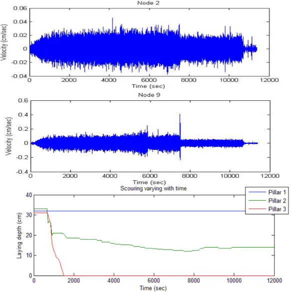
Velocity response data of the bridge during scouring process are collected. Figure 3 shows data from sensor node #2 and node #9. The VSE-15D sensor is used nad it is a servo velocity meter produced by Tokyo Sokushin Co., Ltd. This sensor is very sensitive to detect the low level vibration motion and the linear range (0.2Hz~70Hz) is suite for SHM applications. The total run time on this bridge scouring test is 200 min.(12,000 sec). At t=5800 sec and t=7500 sec significant change of vibration measurement at pier No.3 had been observed from sensor node No.9. Data acquisition system collected all the velocity response of the bridge from all twelve sensors with sampling rate of 200 Hz. Camera was also installed in each of the bridge pier to observe the scouring phenomenon. Figure 3 also plot the scouring depth from the observation. All the test setup will be good for on-line monitoring of the bridge structure. As shown in Figure 3 at pier 3 the laying depth (embedment depth of sand, i.e. 30 cm) significantly reduced at the beginning of the incoming water as compare to the other piers. This si due to the design of the channel to let the scouring phenomenon becomes more concentrated on one single pier.

From the observation of the response measurement in transverse direction (along the channel direction) at t=5800ses and at t=7500 sec some abnormal situation were happened in the bridge structure. This particular time can be used as an index of sever damage of the bridge if one can use these vibration-based monitoring signals. It is important to note that if at t=5800 sec some abnormal phenomenon or features from the response measurement can be extracted through on-line identification, then these features can be used for early warning indices before the significant damage of the bridge. Therefore, on-line system identification techniques from using velocity/

acceleration response become more meaningful if one can detect the abnormal features prior the significant settlement of the bridge pier.

3. METHODOLOGIES OF ON-LINE SYSTEM IDENTIFICATION FROM RESPONSE MEASUREMENTS

In this section three different approaches on on-line monitoring of structural vibration data for operation modal analysis will be discussed which include: the Short Time Fourier Transform method, the Wigner-Ville transformation and the Recursive Subspace Identification algorithm.

3.1 Short Time Fourier Transform (STFT)

To investigate the time-varying characteristics of the processed signal (output only), time-frequency analysis directly from measurements is adopted. STFT uses windowed regular harmonics and function orthogonality to simultaneously extract time-localized components. Mathematically, STFT of a signal x(t) can be expressed as:



 



 X x t w t e dt

t x

STFT{ ( )} (,) ( ) ( ) ^it (1) where w(t) is the window function, commonly a Hamming window or Gaussian "hill"

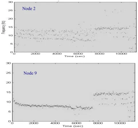
centered around zero, and x(t) is the signal to be transformed. The short-time Fourier transform (STFT) provides one of the techniques to perform the time-frequency analysis of the data. To apply this method to the bridge vibration data the Hamming window length is set to 5.0 sec (1000 points), and with moving window of 2.5 sec (500 points). Data collected from each sensor was calculated individually and plot the time-frequency-amplitude relationship. Figure 4 shows and time-frequency analysis of data from sensor No.2 and No.9 by using STFT method. It is interest to know that at

sec

6000

t and at t 7500secthe significant change of system dominant frequencies

can be clearly identified. This change of system dominant frequencies is inconsistent with the damage of the bridge pier (settlement of bridge pier due to scouring).

3.2 Time-frequency Wigner Ville Transformation

A time-frequency transformation, which does not possess the disadvantage of an additional window, is the Wigner-Ville transformation W(t,):[6]

 

 x t  x t e ^{ } d t

W_xx( , ) 



3.3 Recursive Stochastic subspace Identification (RSSI)

The recursive stochastic subspace identification (RSSI) algorithm is used for conducting operational model analysis through output-only measurements (or ambient vibration). A new RSSI algorithm has been proposed to avoid the use of singular value decomposition [7, 8]. These algorithm consist of two steps: (1) update the LQ decomposition; (2) update the column space of extended observability matrix. The first step implies that the LQ decomposition needs to be updated as long as there is a new set of data provided. The

second step on updating algorithm was proposed how to update the LQ decomposition when appending only one column to block Hankel matrix. To speed up the computation for on-line and almost real time computation, an advanced algorithm to update the LQ decomposition when appending more than one column to block Hankel matrix will be proposed. Procedures for recursive subspace identification are described as follows:

1. To compute the LQ decomposition for the recursive subspace identification algorithm the Givens transformations is used.

2. Considering the recursive identification procedure the new sampling data with the length of columns need to be added to the block Hankel matrix, . In order to remain the same size of Hankel matrix the old data with equivalent length needs to be eliminated.

3. For recursive identification with p-appended data points the update LQ decomposition used the Givens rotation twice at one turn. The second Givens rotation was applied to transform the temporary decomposition into the real LQ

decomposition.

Through this process there is no need to conduct the LQ decomposition on the new Hankel matrix for each recursive procedure which can reduce the computation time to extract the system dynamic characteristics. Detail calculation of RSSI can be found in reference [9]. Figure 6 shows The relationship between the data in moving time window and the required computation time for each data set.

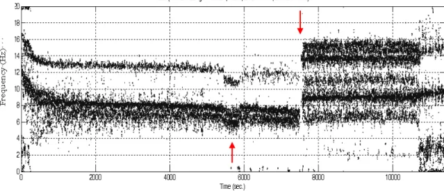
It is important to note that to extract the system dynamic characteristics from the observation matrix, distinguish the true modes from the noise modes becomes a very critical issue. The system order n based on the singular value decomposition (SVD) of observation matrix Ο_i was first determined. Through the use of singular value decomposition (SVD) the system order n can be determined from the singular value greater than the assign value. Then output modal accuracy correlation (OMAC) and weighted phase error (WPE) procedures can sequentially be used, and the true modes can be distinguished from the noise modes [10]. Figure 7 shows the identified time-varying system natural frequencies of the bridge structure by considering all the measurements from the deck to form the data Hankel matrix for RSSI. It is observed that the change of system dominant frequencies in relating to the scouring depth and the pier settlements is closely related. It is important to pointed out that prior to the t=7800 sec (significant settlement at pier No.3) the change of system dominant frequencies can be observed.

The above three time-frequency analyses, STFT, WVD and RSSI, are all in relating to on-line data processing technique. From these analyses a clear picture of time-varying system natural frequencies can be identified. The fundamental frequency of the bridge system was changed from 12 Hz to 7.0 Hz where significant settlement was occurred. These change of system frequencies are in relating the effect of scouring depth. Scouring may change the boundary condition of the bridge pier which may cause the degradation of system natural frequencies. For setting an early warning system on the endangerment of bridge due to scouring, besides the RSSI, more features need to be explored before the significant change of system natural frequencies.

4. DAMAGE DETECTION AND LOCALIZATION

Different from the detection of time-varying system natural frequencies, more

significant features which can not only identify the damage nut also detect the damage locations need to be explored. Through vibration-based monitoring data the on-line damage location was investigated.

4.1 Application of Cross-correlation Function Amplitude Vector

To avoid the limitation of the model-based damage detection techniques and considering the need of on-line damage detection, the concept of cross correlation analysis can be used. One simple approach is to test the cross-correlation from two measurements at the same time. Consider two random signals the correlation,

) ( )

(t and x t

x_{k i} , the correlation coefficient between these two signals is defined as:











T j T

k T

j k kj

d x d

x

d x x

0 2 0

2 0

) ( )

(

) ( ) (













  (3)

where “T” is the time window selected for estimating the correlation coefficient. It is believed that for an intact structural system the correlation coefficient _kj between two measurement nodes, k and j, should be higher than the damage structure. Suppose more than two measurements are taken the concept of cross correlation function amplitude vector (CorV) of the responses of a structure can be used [11]. It is defined the CorV as:

} {r_k1 r_k2 r_k3 r_kn

CorV (4) where r is the maximum value of the cross correlation function between _kl

and t

x_k( ) x_l(t) (l 1,2,3,,n):

dt t

x t T x

R

r l

T

l T k

l kl

kl 1 ( ) ( )

lim ) ) (

max( ^



    (5) Since that the CorV is a vector, so it can be normalized as follows:

12 2( )

) ) (

( ^



i i

jCorV

CorV CorV (6)

It is believed that the correlation coefficient between the measurement locations )

( )

(t and x t

x_{k i} in a structure should be close to one if the structure is not damage.

Otherwise, the correlation coefficient will be low if damage occurred in the structure.

In order to identify and quantify such a damage that occurred in the structure the correlation between two CorV’s is defined:

  





 _{2 2}

2

] ) ( [

)]

( [

] ) ( )

( [

j j

j j

CorV CorV

CorV

CVAC CorV & CVAC[0,1] (7)

where CorV (j) and CorV*(j) indicate the correlation coefficient of two different state, one is the reference state and other is the damaged state (or data calculated from different time period to express the different situation to the reference state). Higher CVAC value indicates higher correlation between the two states.

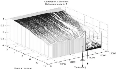
From the monitoring data of bridge scouring test, first, using Eq.(3), the correlation coefficient between two measurement locations is calculated. It is assumed that data from the sensor location No.1 is considered as the reference measurement.

For a fix time window the correlation coefficient between the monitoring data from the reference location and the other measurement location can be generated.

Correlation coefficient with moving time window of 20.0 sec, is generated and shown in Figure 8. It is observed that a significant drop of correlation coefficient with respect to the reference measurement location (sensor No.1) was observed at time t=7800 sec.

which is in consistent with the results from time-frequency analysis. the abnormal of correlation coefficient was also observed between t=6000 sec and t=7800 sec. Based on Eq.(7) CVAC was also calculated with respect to different reference data (measurement location). Figure 9 shows the calculated CVAC as a function of time by considering two different sensing nodes as references. A moving time window with time window of 20 sec was used. The first time window set of the data will be used as the undamaged set of data (or reference). From CVAC value one can detect the abnormal change of CVAC starting at t=6000. sec. which was identified as the prior information (or early warning

message) to the significant change of CVAC which occurred at t=7500 sec. No matter which location was selected as the reference sensor node the CVAC value can still detect the damage. It is important to note that the CVAC can provide an early warning message before the significant change of the system dynamic characteristics (such as the dramatic drop of system dominant natural frequency).

4.2 Application of Proper Orthogonal Decomposition (POD)

Proper orthogonal decomposition is a procedure for extracting a basis for a modal decomposition from an ensemble of signals. If the response signal q_k(t)of a discrete dynamic system with m degree of freedom (d.o.f.) are sampled n times and if the matrix Q is defined as



















) ( )

(

) ( )

(

1

1 1

1

n m m

n

t q t

q

t q t

q











Q (8)

Then the proper orthogonal modes are the eigenvector of ^{G }

 

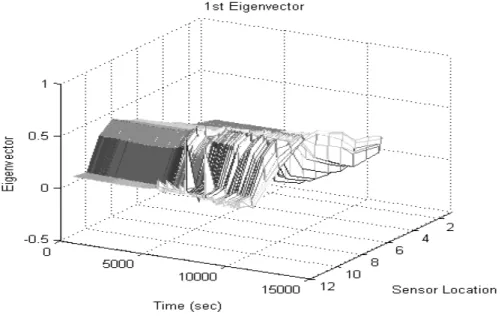
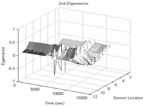
corresponding eigenvalues are the proper orthogonal values. It had been proved that POMs are related to the vibration eigenmodes in some cases. Therefore, the POD should be an alternative way of modal analysis for extracting the mode shapes of a dynamic system. The POD was applied to the dynamic response data collected from the measurements of the bridge scouring test. Figure 10a shows the calculated time-varying first eigenmode. To evaluate the change of eigenmode along the time sequence, the initial calculated eigenmode was selected as the reference one; and then the root-mean-square error of the difference between the reference 1^st eigenmode and the eigenmode calculated from different time window is generated, as shown in Figure 10b. The same analysis can also be calculated using the 2^nd mode information, as shown in Figures 11a and 11b. It is observed that the abrupt change of time can be identified.

4.3 Damage Detection from Novelty Analysis

Different from the CVAC analysis, to conduct the structural damage diagnosis, based on the undamaged data the structural system matrix was estimated as a reference state.

First, the reference data set was collected and the SSI algorithm was applied to estimate the undamaged state of the structural system. Based on the reference data set (the 1^st initial data set is assumed as the reference data), the SSI method is applied to identify the undamaged system transition matrices Φ_k1/kwhich can be computed by exploiting the shift structure of the extended observability matrix.

The novelty analysis on system’s dynamic responses is used to determine the bias of the predict responses if the system significantly deviates from initial baseline condition. The idea is to examine if the Kalman prediction model identified from the reference state data can be applied to newly measured data. Residual error can be estimated by comparing the predicted responses with the measured ones. The k-step state vector and the corresponding prediction error are calculated as:

e_k Y_k Yˆ_k Y_k M_kXˆ_k (8) From the prediction error vectors e_k at any k-th sampling point, the Novelty index

(NI) is defined as either Euclidean Norm or Mahalanobis Norm [12]:

Euclidean Norm: NI_k^E  e_k (9a) Mahalanobis Norm: NI_k^M  e^T_k ^1e_k with yy^T /N (9b) The prediction procedure is performed using the data from the reference and actual states of the structure respectively. In the absence of damage, the level of prediction errors should remain unchanged. Otherwise, the Novelty index will change significantly for the damage case. Besides, the outlier statistical analysis, such as mean and standard deviation of NI, can also give a quantitative assessment of damage.

In Novelty analysis the identified system transition matrix needs to be estimated in advance, and the ordinary Kalman filter can be used to predict the sate. The Kalman filter, in estimating the state consists of two estimates of the state X_k1: (1) a predicted estimate X^ˆ_k1/k of the state X_k1 based on information up to the time

t k

t   (consisting of observations Y₁,,Y_k ); and (2) an update estimate

1 /

ˆ 1



 k

Xk which is obtained at time t (k1)t when a new measurement Y is _k1 observed. For damage estimation the difference between the predicted estimate of state vector, Xˆ_k Φ_{k k}Xˆ_k

/ 1

1 

  and the measurements is calculated. Recursive processing of the measurement data is applied through compute the predicted state and predict the observation Y_k1 and compute the update state. For damage assessment only the predicted measurements are used, the computed update state is only for the estimation of Kalman gain and the prediction error covariance.

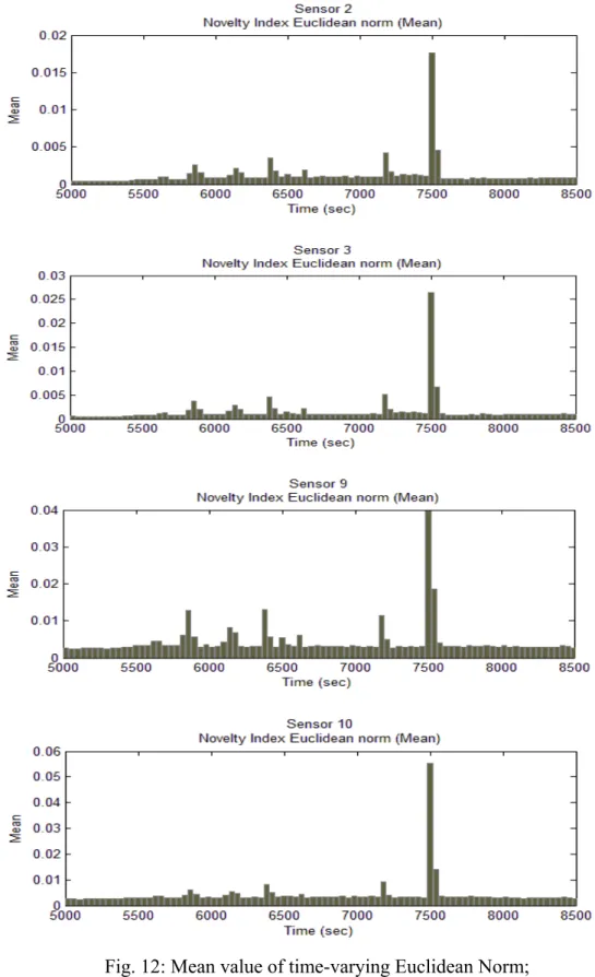
To perform the Novelty analysis using the response measurement of bridge during scouring process, signals collected from all sensors (12 sensing nodes) are collected to form the Hankel matrix with dimension of [12007900]. The time window is set to 40 sec. and with moving window of 40 sec. the first time segment will be used as the undamaged case. Figures 12a and 12b show the plot of the mean value of Euclidean Norm from each window was calculated from sensor node No.2 and No.9 respectively. It is observed that the mean value of Norm for each time window increase significantly at t=6000 sec. (particularly for data from sensor No.9 node) which was identified before the significant change of system dominant frequency. Comparison among the results from RSSI, Novelty analysis and the

vertical deformation measurement at Pier No.3, one can detect the abnormal features from the vibration measurement before the significant settlement of bridge pier occurred. This Novelty analysis can also be used for early warning index.

4.4 Singular Spectrum Analysis for damage detection and early warning

The use of singular spectrum analysis is discussed as an alternative to traditional digital filtering method. Its usefulness has been proven in the analysis of climate and geophysical time series. A description of the method will be given in this session. SSA procedure consists of four steps: (1) embedding, (2) singular value decomposition (SVD), (3) grouping, and (4) reconstruction. The detail description of each step is shown in formal terms as follows [13, 14]:

Step1: Embedding The method starts to produce a Hankel matrix from the time series itself by sliding a window that is shorter in length than the original series.

Firstly, let F  (f₀, f₁,, f_N1) be the time series of length N. And let L be the window length, which is an integer in 1< L<N. Each sliding window vector Xj with length of L would then be derived: Xj =( fj-1, fj , …, fj+L-2 )^T, j = 1, 2, …, K, where K

=N-L+1 is the number of columns. The matrix X = [X1, X2, …, XK] is a Hankel matrix (or called trajectory matrix) since all elements in diagonal i+j=constant are equal.

:

































1 1

1

1 4

3 2

3 2 1

1 2

1 0

N L

L L

K K K

f f

f f

f f

f f

f f

f f

f f

f f X



















(10)

Step2: SVD of the Hankel matrix The Hankel matrix can be represented in the form: X = E1+ E2+…+ Ed, where d is the number of non-zero eigenvalues of theLLmatrix S = X．X^T. The i-th elementary matrix, or called i-th eigentriple, are given by Ei = _i Ui ViT, where₁,₂,..._d are the non-zero eigenvalues of S, in descending order, U₁, U₂, …, U_d are the corresponding eigenvectors, and vectors V_i are derived by Vi=X^T．Ui/ _i , i=1, 2, …,d. The plot of the eigenvalues in descending order is called the singular spectrum and is essential in deciding the index from where to truncate the summation.

Step3: Grouping This step is to decide a parameter r to reconstruct an approximate matrix of X, i.e. X ≈ E1+ E2+…+ Er. The decision making procedure

may varied depending on the objectives of users. For example, if one intends to derive the tendency of the structural response displacement, by which the residual displacement may be clearly indicated, r would be decided as 1, namely the first leading eigentriple.

Step4: Reconstruction The approximate matrix is no longer a Hankel matrix, but an approximated time series may be recovered by taking the average of the diagonals. It is practical to recover the elementary time series for each elementary matrix. These elementary time series (g0, g1, …, gN-1) is also called the principal component. If yij is used to represent the i-th row and j-th column element in any elementary matrix E, the reconstruction algorithm for each principal component can be formulated as follows:

















 











 

















  

  



  

N k P for k y

N

P k R

for R y

R k for k y

g

P N

P k m

m k m R

m

m k m k m

m k m

k

1 2

2 , 1

2 , 1 1

2 ,

1 1 1

1 1 0

1

(11)

where R=min(L,K), P=max(L,K). The smoothed time series is obtained by adding the first r principal components.

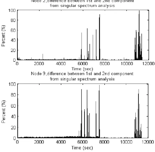
With the concept of moving window (window length=40 sec) the data Hankel matrix was formed. This analysis can be done either for each sensing node or from all recorded sensing nodes. Through SVD the on the data Hankel matrix and eigenvalues were calculated. Figure 13a shows the difference between the first two largest eigenvalues from each of the sensing node. This figure shows that prior to the significant settlement of the bridge pier No.3 at 7=7800 sec, the distinct feature of the difference between two largest eigenvalues can be identified ( at about t=6000 sec).

This feature can be served as an index for early warning. This difference on the first two largest eigenvalues can also be calculate from all set of measurements instead of using data from a single sensing node, as shown in Figure 13b (plot in log sacle).

Through the reconstruction process of signal in SSA by using only the first two largest eigenvales, comparison between the original signal and the reconstructed signal was made. The reconstruction is using the moving window technique by selecting the time window of 40 sec and with moving window of 40 sec. The size of the Hankel matrix is set to 6007951. The root-mean-square (RMS) error between the reconstructed and

recorded signal is plotted and shown in Figure 14. It is observed that the RMS error of the sensor signal from node 9 shows a significant change (around t=5800 sec) before the large settlement occurred. This indication can also provide an early warning index.

5 FIELD EXPERIMENTS

Based on the proposed RSSI-DATA method, applications of the methodology to field test data are conducted. Two field experimental data were collected for this analysis:

a. Vibration measurement of the Nu-Dou old bridge before and during the flood (typhoon) period.

b. Vibration measurement of New Nu-Dow bridge during and after the typhoon period.

Discussions on the results of experiments are shown below:

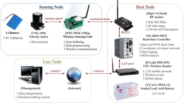
Wireless communication system for data transmission is used in this experiment, as shown in Figure 15. Figure 16 shows the sketch of the bridge. On Sept. 19, 2010 Fananpi typhoon invading I-Lan area. Significan rainfall was observed in the northern part of Taiwan. Figure 17 shows the photo of the bridge in its normal weather condition and in its typhoon period. Application of RSSI-Data to the measurements is conducted during the flood period and after the flood was gone. RSSI-DATA method was applied to the recorded data from sensor node D5H and D14H. It is observed that time-varying system natural frequencies were observed from the data at sensor node D14H, as shown in Figure 18. If the recorded data is re-arranged, as shown in Figure 19, the proposed indices for detection the change of system natural frequencies can also be applied. Figures 20 and 21 show the same analysis of using STFT, WVD, Euclidean norm and percentage change of the 1^st and 2^nd singular spectrum. It is clearly observed that all these indices can detect the change of abnormal condition from the measurements. The old Nu-Dow bridge was tear down due to the newly constructed bridge in its upper stream.

On October 4, 2011, water level at the new Nu-Dow bridge becomes quite high due the heavy rainfall in mountain area of the upper stream. Five sensors were deployed on the new bridge to measure the vibration of the bridge during severe stream flow, as shown in Figure 22. The marked water level during the heavy rainfall induced stream water is at 204.0 meter. On October 13 the water level was dropt to its normal condition, i.e. at 202.7 meter. Figure 23 shows the recorded vibration data of the bridge: one is at the high water level and the other one is at low water level.

SSI-COV was used to identify the system natural frequencies of the bridge under two different operational measurements. Stability diagram is constructed, as shown in Figure 24. It is observed that no change on the system natural frequencies from these two measurements, except that some frequencies can not be detected under the abnormal loading condition.

CONCLUSIONS

Development of structural diagnostic approaches, in-service monitoring of structures with sensor networks may serve an important tool to identify the system modal parameters automatically and evaluate operational health of structures during normal operation condition. Damage detection algorithms depend on the accuracy of the modal parameters estimates and the success of on-line structural health monitoring and damage detection on feature extraction from response data. The main objective of this study on structural health monitoring (SHM) for bridge structure during scouring process is to identify the features from the in-situ operational condition and to detect the changes when damage occurred. Through the experimental study of bridge damage due to scouring the feature extraction techniques were derived and verified.

The feature extraction techniques on time-frequency analysis include:

1. Short Time Fourier Transform, 2. Wigner-Ville distribution,

3. Recursive Stochastic Subspace Identification

These three methods can be applied for on-line feature extraction, and on the identification of time-varying system frequencies. With suitable selection of model parameters one can conduct these analysis in almost real time analysis.

As for damage detection and early warning, distinct feature will be extracted from measurements before the severe damage occurred. Four methods are proposed in this study:

1. Moving time window cross-correlation coefficient, _k,j(X, 0)

2. Generate correlation coefficient between damaged and undamaged cross-correlation function amplitude vector, CVAC.

3. Conduct Novelty analysis to compare the difference between the measurement and the estimated response through Kelman estimator by using the undamaged system

matrix generated from SSI analysis.

4. Difference on the eigenvalues from the Singular Spectrum Analysis.

Through the experimental study on bridge damage caused by scouring in the laboratory, the time-varying dynamic characteristics and the damage features of the bridge can be identified. It is possible to detect the abnormal situation (or features) from the response measurements before the significant damage occurred.

Appendix: Mathematical background of RSSI-DATA

A1. THE CLASSICAL SUBSPACE IDENTIFICATION ALGORITH

Consider a discrete time state-space dynamic system with n DOFs. The system equation can be represented as [15]:

(1a)

(1b)

with . is

called the discrete-time state matrix, is the discrete-time input matrix, is the discrete-time state vector, is the sample time and . is the process noise due to disturbances or modeling error and is the measurement noise due to disturbances or sensor error. For white noise excitation Eq.1 can be replaced by the discrete-time stochastic state space model [15]:

(2a) (2b) where are white noises in stochastic system. The superscript

“s” means “stochastic” and it implicates that the system is excited by stochastic component (noise).

Stochastic Subspace Identification (SSI) using output-only measurement

In stochastic system, using stochastic subspace identification algorithm, the output Hankel matrix can be constructed from the output data and defined as:

(3)

where is the number of block rows which is a user-defined index and must be larger than the order of the system. Since there are only DOFs measured, the output Hankel matrix must contain rows. is the number of block columns of the output Hankel matrix. If the sampling length is equal to then the number should be equal to so that all data are used for analysis. The main theorem of stochastic subspace identification implicates that the extended observability matrix can be found from the result of orthogonal projection. The orthogonal projection can be easily expressed in terms of the following LQ decomposition:

(4a) and

(4b) where is partitions of the lower triangular matrix from LQ decomposition, is the partitions of the orthogonal matrix. This implicates the column space of the extended observability matrix can be obtained from the column space of . Once are obtained from the LQ decomposition of the orthogonal projection, the system parameters can be determined.

Subspace Identification (SI) using Both Input & Output Measurements

The equation, shown in Eq.1, are also named as a discrete-time combined deterministic-stochastic system because it is a combination of a deterministic system and a stochastic system by combining the state and output individually.

Similarly, the input data can be arranged in the Hankel matrix:

(5)

where is the past input Hankel matrix and is the future input Hankel matrix. The matrices and are defined by shifting the border between and one block row down. Moreover, two special Hankel matrices consisting of both input and output data are defined as [15]:

(6) The deterministic state is also divided into past and future parts:

(7) From these definitions, the combined deterministic-stochastic model can be transformed into matrix equations [15]:

(8)

with

(9) (10) where is the low block triangular Toeplitz matrix and is the reversed extended controllability matrix. In above equations, the contribution of the deterministic model is described manifestly and the matrices and substitute the contribution of the stochastic model. If the modal properties (natural frequency,

damping ratio and mode shape) of the structure are needed, the “Multivariable Output-Error State Space” algorithm (MOESP) can be employed to extract the column space of the extended observability matrix from the LQ decomposition of the Hankel matrix [15]:

(11)

And

(12)

Finally, only factor is needed for system identification. Once are obtained from the LQ decomposition of the Hankel matrix in Eq.(11), t the singular value decomposition can be performed, as shown below:

(13) (14) and can be determined from and the modal properties of the system can finally be identified.

A2. RECURSIVE SUBSPACE IDENTIFICATION

One of the advantages of the subspace identification algorithms lies in the use of singular value decomposition (SVD) and LQ decomposition which lead to the stability and reliability of this technique. However, the traditional subspace identification is not suitable for on-line computation because the computational complexity of SVD. To detect the time-varying system the recursive system identification needs to be developed.

Several recursive subspace identification algorithms have been proposed to avoid the use of singular value decomposition [16, 17]. These algorithms always consist of two steps: (1) update the LQ decomposition; (2) update the column space of extended observability matrix. The first step implies that the LQ decomposition needs to be updated as long as there is a new set of data provided. The second step on updating algorithm was proposed how to update the LQ decomposition when appending only one column to block Hankel matrix. To speed up the computation for on-line and almost real time computation, an

advanced algorithm to update the LQ decomposition when appending more than one column to block Hankel matrix will be proposed. Procedures for recursive subspace identification are described as follows:

A. LQ Decomposition and Given Rotations

Consider the LQ decomposition of a matrix is given by:

(15) where is a lower triangular matrix and is an orthogonal matrix ( ). It is assumed which meets the size of the Hankel matrix in the subspace algorithms. As the right columns of consist entirely of zeroes, Eq.(15) can be partitioned as:

(16)

where is a lower triangular matrix, , and

and both have orthogonal rows. is called the thin LQ

decomposition of . If has full rank and it requires that the diagonal elements of are positive and and are unique, but in general is not.

To compute the LQ decomposition for the recursive subspace identification algorithms the Givens transformations is used. A Givens rotation is defined as a matrix of the form [19]:

(17)

with . That is, a Givens rotation matrix is an identity matrix with the following substitutions:

(17a) The product represents a counterclockwise rotation of the column vector

in the coordinate plane of radians and the Givens rotation is

clearly an orthogonal matrix since . It is easy to zero a selected entry in the column vector by multiplying a specific Givens rotation to :

(18)

with , , and . To introduce zeros in a

matrix and make it to become a lower triangular matrix , the matrix should be multiplied by a series of Given rotations at its right side:

(19) The dimension of the Givens rotation is equal to . Eq.(19) can then be represented as the LQ decomposition of :

Let (20) and

(21) Therefore, a matrix can be transformed into a lower triangular matrix through multiplying a series of Givens rotation.

B. Form the Block Hankel Matrix

In the output-only SSI the observability matrix can be extracted from the output block Hankel matrix by using the LQ decomposition and the singular value decomposition:

(22) Similar procedure for the input/output SI was proposed in the Multivariable Output-Error State Space (MOESP) algorithm as [15]:

(23) In this study a new form of block Hankel matrix was proposed for the recursive subspace identification. In the beginning, the block Hankel matrix in Eq.(23) is redefined as:

(24)

where is a block Hankel matrix consist of the columns vectors and each column vector contains the input and output data as:

(25) As mentioned in Eq.(24) if is a rectangular matrix and , the right

columns of the lower triangular matrix form the LQ decomposition of will consist entirely of zeroes. It is useless to compute the excess orthogonal rows (as in Eq.(16)) because only the first columns of the lower triangular matrix is needed to ensuing singular value decomposition. It is feasible to save time by producing an “economic-size” decomposition. Therefore, this study yields the square matrix of to avoid wasting the computation time by giving a relationship between the sampling length r (or now, the length of moving window for updating the LQ decomposition) and the number of block rows i in square matrix

:

(26) From Eq.(26), if the number of input “m” and the number of output “l” are both fixed, then “r” can be determined by assigning the number of block rows “i”. Since now

is a square matrix, the LQ decomposition of can be defined as:

(27) where is a square and lower triangular matrix and is also square and orthogonal matrix.

Based on the result of LQ decomposition of Hankel matrix , firstly, a Givens rotations is used to transform the first columns of into an upper triangular matrix:

(28)

where is an upper triangular matrix. Since and are both orthogonal, the product of them must be orthogonal:

(29) Based on the criteria of Eq.(29), it can be proved that and , then Eq.(28) can be replaced by:

(30)

From the first data set, by using the Givens rotation , the LQ decomposition of block Hankel matrix , as shown in Eq.(27), can be replaced as:

(31) From which and can be estimated through the Givens rotation of ,

respectively.

C. Methodology for Recursive Computation

To consider the recursive identification procedure, if the new sampling data with the length of are added to the block Hankel matrix , the old data with equivalent length will be eliminated. The updated block Hankel matrix and its LQ decomposition is re-defined as:

(32) How to compute the new decomposition by using the new sampling data and the old decomposition results, , is the crucial issue in recursive identification.

The Givens rotations actually decouples the LQ decomposition of that the first columns of is returned to the original form of block Hankel matrix

. Remove from , Eq.(32) implies the remains can be represent as:

(33) where is orthogonal, and is close to be a lower triangular matrix. To accommodate the recursive procedure, the new data set is appended to the remains:

(34) where is orthogonal, and is close to be a lower triangular matrix. To make Eq.(34) become a complete LQ decomposition the Givens rotations is used again to transform the

into a real lower triangular matrix :

(35) For recursive identification with p-shift data point, Figure A1 show the summary of the related equations which were used in two consecutive time window. In summary, the first Givens rotations decoupled the old LQ decomposition so that the old data can be deleted. After appending the new data, the second Givens rotations as applied which make the temporary decomposition become a real LQ decomposition.

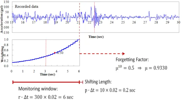
Moreover, a forgetting factor μ can also be used to improve the convergence of the recursive subspace identification by multiplying it to the past data sets in Eq.(34):

(36) The implementation of forgetting factor is to use the concept of fading memory by decreasing the weight of data points which were away from the current data. The idea of fading memory on the previous data can be used especially to detect the abrupt change of system modal parameters. For example, if the length of moving window is

assumed as and the shifting length is

(r and p indicate the number of data point), and the forgetting factor can be determined from with μ=0.9330, and then the weighting factor can be calculated and applied to the data set of the specified time window, as shown in Figure A2.

Figure A1: Correlation of Hankel matrix in recursive formulation from Data Set 1 to Data Set 2 (with shift p step).

Figure A2: Weighting factor for window length of 6 sec. applied on data between 15 sec and 21 sec.

REFERENCES

[1] Fukui, j. and Otuka, M. “Inspection method on scour condition around existing bridge piers,” First International Conference on Scour Foundation, 2002.

[2] Lagasse, P.F., Zevenbergen, L.W., Zachman, D.W., “Bridge scour and stream instability countermeasures,“ Report FHWA-NH-01-003 Federal Highway

Administration, Hydraulic Engineering Circular No.23, 2001.

[3] Reda Taha, M.M., A. Noureldin, J.L. Lucero, and T.J. Baca, Wavelet transform for structural health monitoring: A compendium of uses and features. Structural Health Monitoring, 2006. 5(3): p. 267-295.

[4] Yen, G.G. and K.-C. Kuo, Wavelet packet feature extraction for vibration monitoring. IEEE Transactions on Industrial Electronics, 2000. 47(3): p.

650-667.

[5] Han, J.G., W.X. Ren, and Z.S. Sun, Wavelet packet based damage identification of beam structures. International Journal of Solids and Structures, 2005. 42(26): p.

6610-6627.

[6] P.G. Baum, “T time-filtered Wigner transformation for use in signal analysis,”

Mechanical Systems and Signal processing 16(6), 2002, pp:955-966.

[7] Peter Van Overschee and Bart De Moor, Subspace identification for linear systems:

Theory-implementation and application, Kluwer Academic Publisher, Dordrecht, The Netherlands:, 1996.

[8] De Cock K., Mercre G., De Moor B. “Recursive subspace identification for in-flight modal analysis of airplanes,” Proc. Of the Inter. Conf. on Noise and Vibration Engineering (ISMA 2006), Leven, Belbium, Sept., 2006, pp:1563-1577.

[9] Chin-Hsiung Loh, Jian-Huang Weng, Yi-Cheng Liu, Pei-Yang Lin and

Shieh-Kung Huang, “Structural Damage Diagnosis Based on On-line Recursive Stochastic Subspace Identification,” Accepted for publication in J. Smart

Materials and Systems 2011.

[10] J. H. Weng, C. H. Loh and J. N. Yang, “Experimental study of damage detection by data-driven subspace identification and finite element model updating,” J. of Structural Engineering, ASCE, 135(12), 2009. pp:1533-1544,

[11] Zhichun Yang, Zhefeng Yu and Hao Sun, “On the cross correlation function amplitude vector and its application to structural damage detection,” Mechanical Systems and Signal processing 21, 2007, pp: 2918-2932.

[12] Ai-Min Yan, Pascal De Boe and Jean-Claude Golinval, “Structural damage diagnosis by Kalman model based on stochastic subspace identification,” J. of Structural Health Monitoring, Sage publication, Vol 3(2): 2004, pp:001-119.

[13] Golyandina, N., Analysis of time series structure: SSA and related techniques.

2001, Boca Raton, Fla. :: Chapman & Hall/CRC.

[14] Alonso, F.J., J.M. Del Castillo, and P. Pintado, “Application of singular spectrum analysis to the smoothing of raw kinematic signals”, Journal of Biomechanics, 2005. 38(5): 1085-1092.

[15] P. Van Overschee and B. De Moor, Subspace identification for linear systems:

Theory-Implementation-Application. (1996), Dordrecht, Netherlands: Kluwer Academic Publishers.

[16] J. Willems, (1987). From time series to linear systems, Automatica, Part I:

22(5), 561-580 (1987); 1986; Part II: 22(6), 675-694, 1986; Part III: 23(1), 87-115, 1987.

[17] H. Oku, H. and Kimura, Recursive 4SID algorithms using gradient type subspace tracking, Automatica (2002); 38, 1035-1043.

[18] I. Goethals, L. Mevel, A. Benveniste, and B. De Moor, Recursive output only subspace identification for in-flight flutter monitoring, Proc. of the 22^nd International Modal Analysis Conference (2004), Dearborn, Michigan.

[19] G.H. Golub and C.F. Van Loan. Matrix computations (1996), 3^rd edition, John Hopkins University Press, Baltimore MD.

[20] J.N. Juang, Applied system identification (1994). Englewood Cliffs, NJ, USA:

Prentice Hall.

■ ■ ■ ■ ■

■ ^■ ■ ■ ^■ ■ ■ ^■ ■ ■ ^■ ■

■ ^■ ■ ■ ^■ ■ ■ ^■ ■ ■ ^■ ■

■ ■ ■ ■ ■ ■ ■

Fig.1: Sketch and dimension of the bridge test specimen

Fig. 2: Photos of the bridge test site and the test specimen, (a) before scouring test, (b) under scouring test, (c) after scouring test.

Fig. 3: Recorded velocity response from node 1 and node 9 from the bridge scouring test on date 2011-01-26. The observation of scouring depth from each pier is also plotted for comparison.

Fig. 4: Time-frequency analysis from data at node 1 and node 9 by using STFT

Fig. 5: Wigner-Ville transformation of signals from record at sensor Node 2 and Node 9

Node 2

Node 9 Node 2

Node 9

Fig. 6: The relationship between the data in moving time window and the required computation time for each data set.

Fig. 7: Identified time-varying system natural frequencies using RSSI algorithm (Window length = 5 (sec) OMAC=0.98, SVD=0.15, N_row=50).

Time-sec (Data point) 1^st Data Set

2^nd Data Set

3^rd Data Set

t r

pt pt

Computation Time (sec)

0

Computation time for 1^st data set

Computation time for 2^nd data set

pt pt

Computation time for 3^rd data set

……

Delay Time (Computation time

vs. Data run time)

Fig. 8: Plot the correlation coefficient with respect to sensor location and time (use sensor 1 data as the reference)

Fig.9: Plot of CVAC with respect to time; (a) consider sensor node No.1 as a reference, (b) consider sensor node No.6 as a reference

Fig. 10a: Calculated 1^st eigenmode from Proper Orthogoanl Decomposition.

Fig. 10b: Root-mean-square value of the difference between reference eigenmode and the eigenmode calculated from different time window.

Fig.11a: Calculated 2^nd eigenmode from Proper Orthogoanl Decomposition.

Fig. 11b: Root-mean-square value of the difference between reference eigenmode and the eigenmode calculated from different time window.

Fig. 12: Mean value of time-varying Euclidean Norm;

(a) response at Node 2, and (b) response at Node 9.

Fig. 13a: Difference between the 1^st and 2^nd eigenvalue-ratio from Singular Spectrum Analysis on each measurement (for Nodes 3, 6, and 9).

Fig. 13b:Difference between the 1^st and 2^nd eigenvalue from Singular Spectrum Analysis on all set of measurements.

Fig. 14: Plot of RMS error between the measurement and the prediction using the reconstruction (from the two largest eigen values) wave forms of SSA.

Figure 15: Wireless data communication setup for field ambient vibration measurements.

Figure 16: The sensor locations along the bridge deck are also shown (in transverse direction)

Figure 17: Photos of the Nu-Dow old bridge before and during the typhoon period.