應用於地面數位電視廣播系統之時序同步化設計

(1)

(2)

(3)

Timing Synchronization for DVB-T System

Student : Cheng-Wei Kuang Advisor : Dr. Chen-Yi Lee

Institute of Electronics Engineering

National Chiao Tung University

ABSTRACT

The synchronization of symbol timing and sampling clock is very important for the OFDM communication system. In this thesis, a whole timing synchronization scheme including symbol synchronization and sampling clock synchronization is presented. The DVB-T (Digital Video Broadcasting – Terrestrial) system is chosen for the research topic. A complete simulation platform which contains transmitter, channel and receiver is built in Matlab. The overview of DVB-T system is presented first. Then the various channel distortions like multipath fading, Doppler, CFO and SCO will be analyzed clearly.

Employing flat peak period decision, the blind Mode/GI detection is exploited as the first stage of synchronization. A detail comparison of different coarse symbol synchronization algorithms is then presented. For more accurate symbol timing, we will illustrate the proposed low complexity fine symbol synchronization with new peak detection strategy. In sampling clock synchronization, a proposed resampler combining interpolator with decimator can reduce nearly half of power consumption. Subsequently, a SCO estimation based on LLS algorithm with the multi-stage tracking loop is proposed which improves the conventional designs. At last of this thesis, the architecture design of each block is presented respectively.

(4)

List of Tables

TABLE 1.1COMPARISON OF EACH DTV BROADCASTING STANDARD... 3

TABLE 1.2COMPARISONS OF DVB-T,DVB-S AND DVB-C... 3

TABLE 2.1DECIMATION CONTROLLER... 43

TABLE 2.2SIMPLIFIED DECIMATION CONTROLLER... 43

TABLE 3.1REQUIRED C/N FOR NON-HIERARCHICAL TRANSMISSION... 60

TABLE 3.2COMPARISONS BETWEEN PROPOSED AND CONVENTIONAL FINE SYMBOL SYNCHRONIZATION... 75

TABLE 3.3JOINT SCO AND CFO ESTIMATION (ONE SHOT) ... 78

TABLE 3.4SNR LOSS IN STATIC GAUSSIAN,RICEAN AND RAYLEIGH CHANNEL... 83

(7)

List of Figures

FIG 1.1FUNCTION BLOCK DIAGRAM OF DVB-T SYSTEM... 4

FIG 1.2FRAME STRUCTURE... 6

FIG 2.1ISI-FREE REGION... 9

FIG 2.2PHASE ROTATION OF SYMBOL TIMING OFFSET ε=2 AND ε=5 ... 10

FIG 2.3MAPPING CONSTELLATION... 11

FIG 2.4SAMPLING CLOCK OFFSET... 12

FIG 2.5PHASE ROTATION BETWEEN CONSECUTIVE OFDM SYMBOLS... 12

FIG 2.6PHASE ROTATION DUE TO TIMING DRIFT... 14

FIG 2.7PERIODIC FLAT PEAK AREA... 17

FIG 2.8DELAYED PEAK OF MOVING SUM... 19

FIG 2.9FOUR MODES OF SCATTERED PILOT POSITION... 21

FIG 2.10EFFECTIVE CHANNEL IMPULSE RESPONSE DUE TO INACCURATE FFT WINDOW... 22

FIG 2.11STRUCTURE OF FINE SYMBOL SYNCHRONIZATION... 23

FIG 2.12DOWNSAMPLING OF CHANNEL FREQUENCY RESPONSE... 24

FIG 2.13 ZERO-PADDING OF CHANNEL FREQUENCY RESPONSE... 24

FIG 2.14PROPOSED LOW COMPLEXITY FINE SYMBOL SYNCHRONIZATION... 25

FIG 2.15STRUCTURE OF SAMPLING CLOCK SYNCHRONIZATION... 26

FIG 2.16PHASE ROTATION BETWEEN TWO CONSECUTIVE SYMBOLS... 28

(8)

FIG 2.18LINEAR LEAST SQUARE LINE... 30

FIG 2.19IDEAL INTERPOLATOR... 33

FIG 2.20COEFFICIENTS OF h_n( )µ USING SINC FUNCTION... 34

FIG 2.21FREQUENCY RESPONSE OF KAISER WINDOW WITH DIFFERENT VALUES OF β ... 35

FIG 2.22FREQUENCY RESPONSE OF KAISER WINDOW WITH DIFFERENT TAPS OF M... 36

FIG 2.23FREQUENCY RESPONSE OF 61-TAP SINC FUNCTION,9-TAP SINC FUNCTION AND SINC FUNCTION TRUNCATED BY KAISER WINDOW... 38

FIG 2.24INTERPOLATION CONTROL... 39

FIG 2.25PARAMETER COMPUTATION IN TIMING PROCESSOR... 41

FIG 2.26STRUCTURE OF 8-TAP RESAMPLER... 44

FIG 2.27PI LOOP FILTER... 45

FIG 2.28CONVERGENCE SPEED OF SYNCHRONIZATION CONSIDERING TPS FRAME... 47

FIG 2.29OVERALL SYNCHRONIZATION SCHEME... 48

FIG 3.1BLOCK DIAGRAM OF SIMULATION PLATFORM... 49

FIG 3.2OVERVIEW OF RECEIVER DESIGN... 50

FIG 3.3STRUCTURE OF INNER RECEIVER... 51

FIG 3.4ISI EFFECT ON CFO ACQUISITION... 52

FIG 3.52D INTERPOLATION IN EQUALIZER DESIGN... 54

FIG 3.6BASEBAND EQUIVALENT CHANNEL MODEL OF DVB-T SYSTEM... 54

FIG 3.7CHANNEL RESPONSE OF RICEAN CHANNEL (K=10DB) AND RAYLEIGH CHANNEL... 56

FIG 3.8DOPPLER FREQUENCY SPREAD MODEL... 57

FIG 3.9JAKES’ SPECTRUM WITH f_d_max =10Hz ... 58

FIG 3.10FLAT PEAK AREA IN MODE/GI DETECTION... 62

FIG 3.11FALSE MODE/GI DETECTION RATE VERSUS SNR... 62

FIG 3.12HISTOGRAM OF ESTIMATED SYMBOL OFFSET IN GUASSIAN CHANNEL... 64

(9)

FIG 3.14HISTOGRAM OF ESTIMATED SYMBOL OFFSET IN RAYLEIGH CHANNEL... 65

FIG 3.15FALSE DETECTION RATE OF SCATTERED PILOTED MODE DETECTION... 67

FIG 3.16ESTIMATED CHANNEL IMPULSE RESPONSE IN GAUSSIAN CHANNEL... 68

FIG 3.17PATH DELAY ESTIMATION IN GAUSSIAN CHANNEL... 69

FIG 3.18ESTIMATED CHANNEL IMPULSE RESPONSE IN RICEAN CHANNEL... 70

FIG 3.19PATH DELAY ESTIMATION IN RICEAN CHANNEL... 71

FIG 3.20ESTIMATED CHANNEL IMPULSE RESPONSE IN RAYLEIGH CHANNEL... 72

FIG 3.21PATH DELAY ESTIMATION IN RAYLEIGH CHANNEL... 73

FIG 3.22FINE SYMBOL SYNCHRONIZATION... 74

FIG 3.23PROPOSED LOW COMPLEXITY FINE SYMBOL SYNCHRONIZATION... 75

FIG 3.24MSE OF FIR INTERPOLATION... 76

FIG 3.25SCO TRACKING... 79

FIG 3.26SCO TRACKING WITH DIFFERENT PARAMETER... 80

FIG 3.27TWO-STAGE SCO TRACKING... 80

FIG 3.28OVERALL SYSTEM PERFORMANCE IN STATIC GAUSSIAN CHANNEL... 81

FIG 3.29OVERALL SYSTEM PERFORMANCE IN STATIC RICEAN CHANNEL... 82

FIG 3.30OVERALL SYSTEM PERFORMANCE IN STATIC RAYLEIGH CHANNEL... 82

FIG 3.31OVERALL SYSTEM PERFORMANCE IN RAYLEIGH CHANNEL WITH DOPPLER FREQUENCY 70HZ... 84

FIG 4.1ARCHITECTURE OF MODE/GI DETECTION... 85

FIG 4.2ARCHITECTURE OF COARSE SYMBOL SYNCHRONIZATION (MMSE) ... 86

FIG 4.3ARCHITECTURE OF PRE-FFTAFC ... 86

FIG 4.4ARCHITECTURE OF SCATTERED PILOT MODE DETECTION... 87

(10)

Chapter 1 Introduction

1.1 Motivation

Synchronization is one of the most important things in a communication system. In the mobile wireless channel, transmitted data suffers from several kinds of distortions caused by multipath fading, Doppler spread, AWGN, carrier frequency offset and sampling clock offset. These effects raise the difficulty of synchronization. In OFDM transmission systems, the task of synchronization consists of carrier frequency synchronization and timing synchronization. Timing synchronization is divided into symbol synchronization and sampling clock synchronization. The purpose of symbol synchronization is to find the correct position of symbol boundary. The inaccurate symbol timing can cause ISI that destroys the orthogonality of subcarriers, which degrades the system performance much. The objective of sampling clock synchronization is to adjust sampling clock frequency in the receiver. The sampling clock offset leads to the symbol timing drift. In the broadcasting communication system, the timing drift problem is more critical with respect to other packet-based system since the incoming data exists all the time. The timing drift can cause severe ISI effect if we do not perform sampling clock synchronization. In order to solve the timing synchronization problem, we choose the DVB-T (Digital Video Broadcasting – Terrestrial) system as the research topic. A complete timing synchronization scheme for DVB-T system will be proposed in this thesis.

(11)

1.2 Introduction to ETSI DVB-T Standard

In recent years, DTV (Digital TV) is widely adopted as the next-generation video broadcasting transmission technology. DTV can provide higher A/V quality and less transmission noise than conventional analog TV. The current developed DTV standards consist of DVB (Digital Video Broadcasting) in Europe, ATSC (Advanced Television Systems Committee) in U.S., ISDB (Integrated Services Digital Broadcasting) in Japan and DMB (Digital Multimedia Broadcasting) in China. The transmission modes of DTV include direct satellite broadcasting, cable and terrestrial broadcasting (over-the-air). In terrestrial broadcasting, particularly, video signal is transmitted against severer channel distortions such as multipath fading, co-channel interference and adjacent-channel interference. Since broadcasting transmission system is usually designed to operate within the UHF spectrum allocation for analogue transmissions, it has to provide sufficient protection against high levels of co/adjacent-channel interference emanating from existing PAL (Phase Alternative Line) / SECAM (SEquentiel Couleur Avec Memoire or sequential color with memory) services. Therefore, it is clearly that the terrestrial broadcasting has more challenges in research. The relative materials of terrestrial broadcasting systems are listed in Table 1.1

Standard DVB-T ATSC ISDB-T DMB-T

Full name Digital Video

Broadcasting for Terrestrial Advanced Television Systems Committee Integrated Services Digital Broadcasting for Terrestrial Digital Multimedia Broadcasting for Terrestrial

Modulation OFDM 8-VSB(Vestigial

Sideband)

OFDM OFDM

(12)

Table 1.1 Comparison of each DTV broadcasting standard

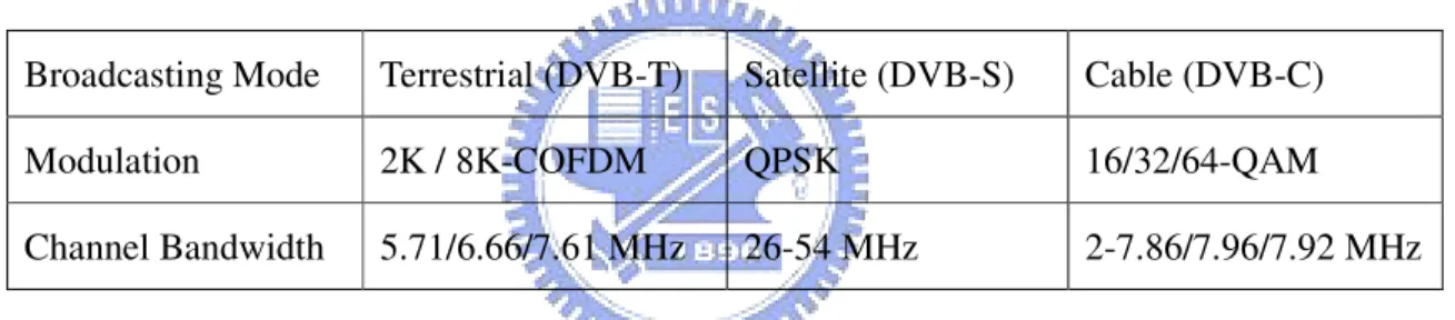
Terrestrial Digital Video Broadcasting (DVB-T) [1] has been subject to technical discussion for many years and undoubtedly been shown as a great success in delivering high quality and standard quality digital television by terrestrial means. DVB-T standard has been produced by European Telecommunication Standard Institute (ETSI) in Aug, 1997, and the second version is released in Jan, 2001. Although originating in Europe, it has been introduced in many countries around the world such as Taiwan. There are two other standards of different broadcasting modes, i.e., DVB-C (cable) and DVB-S (satellite) being specified by ETSI simultaneously. Both DVB-C and DVB-S are simpler system compared to DVB-T as listed in Table 1.2.

Broadcasting Mode Terrestrial (DVB-T) Satellite (DVB-S) Cable (DVB-C)

Modulation 2K / 8K-COFDM QPSK 16/32/64-QAM

Channel Bandwidth 5.71/6.66/7.61 MHz 26-54 MHz 2-7.86/7.96/7.92 MHz

Table 1.2 Comparisons of DVB-T, DVB-S and DVB-C

DVB-S has high channel bandwidth (26-54 MHz) and uses QPSK modulation. DVB-C applies 16/32/64 QAM modulation without convolutional code because of lower channel noise and interferences. Nevertheless, in order to provide the high data rate required for video transmission and resist severe channel distortion in DVB-T, concatenated-coded Orthogonal Frequency Division Multiplexing (OFDM) has been adopted into DVB-T in particular. OFDM is a very popular technology today due to its high data rate transmission capability with high bandwidth efficiency and its robustness to multipath distortion. It has been also chosen as the transmission technique of other communication systems such as ADSL, VDSL, XDSL, DAB and IEEE802.11a/g.

(13)

broadcasting channel, many parameters of OFDM for DVB-T can be dynamically changed according to channel conditions. The number of OFDM subcarriers can either be 2048 (2K) or 8192 (8K) so that the desired trade-off can be made between inter-symbol-interference (ISI) and Doppler spread. In the 2K mode, wide subcarrier spacing can reduce the distortion caused by Doppler frequency spread. In the 8K mode, long OFDM symbol duration can overcome large multipath fading. Other parameters like guard interval length, constellation mapping mode and coding rate of Viterbi can be also properly decided up to the broadcasting channel condition of the local area.

The transmission system is shown in Fig 1.1. It contains the blocks for source coding, outer coding and interleaving, inner coding and interleaving, mapping and modulation, frame adaptation and OFDM transmission.

Fig 1.1 Function block diagram of DVB-T system

In the case of two-level hierarchy, the functional block diagram of the system must be expanded to include the modules shown in dashed in. The splitter separates the incoming data stream into the high-priority and the low-priority stream. These two bitstreams are mapped onto the signal constellation by the mapper and therefore the modulator has a corresponding

(14)

number of inputs.

As in the baseline systems for satellite and cable, source coding of video and sound is based on the ISO-MPEG2 standards. After the MPEG2 Transport Multiplexer, the packet may optionally be split into two data streams of different priority in case of hierarchical modulation/channel coding. Subsequently, a Reed Solomon (RS) shortened code (204, 188 t = 8) and a convolutional bytewise interleaving with depth I = 12 is applied to the error protected packets (outer interleaving). As Fig 1.1, the outer interleaver is followed by the inner coder. This coder is designed for a range of punctured convolutional codes (Viterbi), which allows code rates of 1/2, 2/3, 3/4, 5/6 and 7/8. If two-level hierarchical transmission is used, each of two parallel channel encoders has its own code rate. Afterward, the inner interleaver is block based bitwise interleaving.

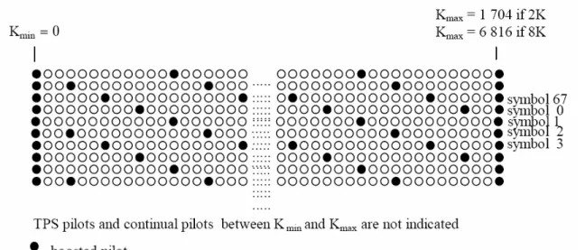
The system uses OFDM transmission. All data carriers in one OFDM symbol are either QPSK, 16-QAM, 64-QAM, non-uniform-16-QAM or non-uniform-64-QAM. In addition to the transmitted data, an OFDM symbol contains scattered pilots, continual pilots and TPS (Transmission Parameter Signaling) pilots. These reference signals can be used for synchronization, channel estimation and transmission mode verification. The OFDM frame consists of 68 OFDM symbols and four frames constitute one super-frame. The frame structure involving distribution of scattered pilots is shown in Fig 1.2. Scattered pilots insert every 12 subcarriers and have an interval of 3 subcarriers in the next adjacent symbol. Continual pilots locate at fixed indices of subcarrier, which contains 177 pilots in 8K mode and 45 in 2K mode. Both scattered pilots and continual pilots are transmitted at a boosted power level of 16/9 whereas the power level of other symbols is normalized to 1.

(15)

Fig 1.2 Frame structure

The TPS carriers are used for the purpose of signaling parameters related to the transmission scheme, i.e. to channel coding and modulation. The TPS is defined over 68 consecutive OFDM symbol and transmitted in parallel on 17 TPS carriers for the 2K mode and on 68 carriers for the 8K mode. Each OFDM symbol conveys one TPS bit which is differentially encoded in every TPS carriers. The TPS information contains frame number, constellation, hierarchy, code rate, guard interval, transmission mode and BCH error protection code. Unlike scattered and continual pilots, TPS pilots are transmitted at the normal power level of 1 with DBPSK modulation. The values of scattered pilots, continual pilots and

TPS pilots are derived by PRBS sequence (X11+X2+1). The guard interval may have four

values, i.e. 1/4, 1/8, 1/16 and 1/32. Guard interval 1/4 would occupy 25% of the usable transmission capacity and hence only be used in case of SFN operation with long distances between transmitter sites. In the case of smaller transmitter distances (local SFN) or non-SFN operation the smaller values of guard interval can be selected. In conclusion, DVB-T system has good flexibility for various transmission conditions, so that it becomes a successful technology for video broadcasting.

(16)

1.3 Thesis Organization

This thesis consists of 5 chapters. The reader is assumed to be familiar with OFDM theory and thus we’ll just focus on timing synchronization of DVB-T system. The effect of timing error and the corresponding synchronization algorithms will be introduced in chapter 2. Chapter 3 provides the overview of simulation platform and we will explain the main blocks and the channel model. The simulation results and comparisons will be presented in this chapter. In chapter 4, we present the architecture design and discuss the considerations about hardware implementation. Finally, conclusion and future work are made in chapter 5.

(17)

Chapter 2 Timing Synchronization Algorithms

2.1 Introduction to Timing Offset

In OFDM system, timing offset would cause inter-symbol interference (ISI) which destroys the orthogonality of subcarriers. The timing offset can be divided into two parts: symbol timing offset and sampling clock offset. The symbol timing offset occurs when symbol synchronization finds incorrect OFDM symbol boundary, and sampling clock offset is caused by the difference between the sampling frequencies of the digital-to-analog converter (DAC) and the one of the analog-to-digital converter (ADC). Sampling clock offset can also lead to symbol timing drift. Unlike other packet based communication system such as 802.11a, DVB-T system is a continuous-data transmission. Therefore, sampling clock offset is a critical problem to be solved.

2.1.1 Effect of Symbol Timing Offset

The symbol synchronization of the OFDM system is to find the start of OFDM symbol,

i.e. the FFT window position. Just as what is shown in Fig 2.1, we call ∆ the ISI-free region.

If the estimated start position of OFDM symbol is located within the ISI-free region, data will not be affected by inter-symbol interference (ISI). The effect of phase rotation caused by symbol timing offset can be easily corrected after FFT.

(18)

Fig 2.1 ISI-free region

Assume x(n) represents received data in time domain, X(k) is subcarrier after FFT

operation for x(n) with perfect symbol timing, and X k^( ) denotes subcarrier after FFT

operation with symbol timing offset

ε

in the ISI-free region. The detail equations are

demonstrated as follows. 1 ₂ 0 ( ) N ( ) i kNn n X k − x n e− π = = (2.1) 1 ^ ₂ 0 ( ) N ( ) i knN n X k − x n e− π +ε = = (2.2) 1 ^ 2 2 0 ( ) ( ) n N _i _k _i _k N N n X k − x n e− π e− π ε = = (2.3) ^ 2 / ( ) ( ) i k N X k =X k e π ε (2.4)

where k represents the subcarrier index, n denotes sample index in time domain, and N is the

number of subcarriers in an OFDM symbol. Note the last term _ei2πkε/N_{in Eq(2.4), which}

exhibits the phase rotation. Therefore, we can conclude that the effect of symbol timing offset in the ISI-free region is phase rotation and unchanged magnitude of subcarrier, which can be compensated by equalizer completely. The phase rotation effect is shown in Fig 2.2. Fig 2.2(b)

depicts the condition of symbol timing offset ε = 2 while Fig 2.2(c) shows the condition of

ε = 5. As symbol timing offset ε is lager, the phase variation is severer. The additional

variance of channel response due to timing error will increase the difficulty of channel estimation. In order to ease the load of channel estimation unit, the symbol timing effect should be as small as possible even the phase rotate effect can be completely corrected in

(19)

theory.

(a) Symbol timing offset ε in the ISI-free region

0 200 400 600 800 1000 1200 1400 1600 1800 -4 -3 -2 -1 0 1 2 3 4 subcarrier ph as e

Phase rotation with symbol timing offset=2

0 200 400 600 800 1000 1200 1400 1600 -3 -2 -1 0 1 2 3 subcarrier ph as e

phase rotation of symbol timing offset=5

(b) Phase rotation due to symbol timing offset=2 (c) Phase rotation due to symbol timing offset=5 Fig 2.2 Phase rotation of symbol timing offset ε=2 and ε=5

On the other hand, if the estimated start position locates out of ISI-free region, the sampled OFDM symbol will contains some samples that belong to previous symbol or following symbol, which leads to the dispersion of signal constellation (ISI) and reduce system performance much. Therefore, the objective of symbol synchronization, first of all, is to avoid the estimated symbol boundary lying in ISI region and subsequently reduce the symbol timing offset as far as possible. The relative mapping constellations are depicted in Fig 2.3. Fig 2.3(a) shows the phase rotation effect due to symbol timing offset of 5 samples while Fig 2.3(b) shows the ISI effect which destroys the signal constellation heavily.

(20)

(a) Symbol offset 5 samples in the ISI-free region (b) Symbol offset 5 samples in the ISI region Fig 2.3 Mapping constellation

2.1.2 Effect of Sampling Clock Offset

The sampling clock errors include the clock phase error and the clock frequency error. The effect of clock phase error is similar to the effect of symbol timing offset and hence we can regard the clock phase error as a fractional part of symbol timing offset. The major impact of sampling clock error is clock frequency error which causes phase rotation in frequency domain and symbol timing drift in time domain. We call the sampling clock frequency error “sampling clock offset (SCO)”.

Sampling clock offset causes sampling timing change at every sample interval as shown in Fig 2.4. For example, if the sampling clock frequency is 8MHz, sampling clock offset is 10ppm, then the symbol timing has a drift of about 80 samples per second. Obviously, SCO is an important issue in broadcasting transmission system like DVB-T. Ignoring sampling clock synchronization would lead to severe timing drift.

(21)

Fig 2.4 Sampling clock offset

Similar to symbol timing offset, sampling clock offset causes phase rotation in frequency domain. Furthermore, the amount of phase rotation is monotonous increasing as the symbol is conveying as shown in Fig 2.5.

Fig 2.5 Phase rotation between consecutive OFDM symbols

To prove the phase rotation of SCO, we consider an OFDM system using IFFT with

N-points. Each OFDM symbol consist of K (K < N) data subcarrier, al,k , where l denotes the

OFDM symbol index and k denotes the subcarrier index, -K/2≤ k ≤ K/2-1, T is the sampling

clock period and Ng is the number of guard interval samples. Then one OFDM symbol has

total Ns samples, Ns is equal to N + Ng. The transmitted complex baseband signal for l-th

(22)

2 ( ( ) ) / 2 1 , / 2 1 ( ) g s j k t N l N T K NT l k k K s t z e N π − + ⋅ − =− = ⋅ (2.5)

In receiver, we assume that the carrier frequency is f’ and sampling clock is T’.

Therefore the carrier frequency offset f∆ and the relative sampling clock offset ζ are

designated as ' f f f ∆ = − (2.6) ( ' ) /T T T ζ = − (2.7)

The l-th received symbol after sampling with the sampling clock T’ and removing the guard interval can be represented as

2 ( ( ) ) / 2 1 2 , / 2 2 2 / 2 1 ₍₁ ₎ ₍ ₎ 2 ( )(1 ) 2 (1 ) , / 2 1 ( ) ( ) 1 _{( )} n g s n g s g s j k t N l N T K j ft NT l l k l k K j kn j k K _N _{l N} j f N l N T j fn T _N _N l k l k K r n e a e v n N e e a e e v n N π π π _ζ π _ζ π ζ π ζ − + ⋅ − ∆ =− − ₊ _{+ ⋅} ∆ + ⋅ + ∆ + =− = + = ⋅ + (2.8)

where tn = (Ng+lNs)T’ + nT’ and ( )v n is the complex Gaussian noise. Demodulation of the l

received samples via FFT yields the data symbol in frequency domain, zl,k.

1 2 / , 0 2 ₍ ₎ 2 ( )(1 ) , ( ) ( ) g s g s N j kn N l k l n k j N l N j f N l N T _N l k l z r n e e e a ICI n k π π _ζ π ζ _α − − = + ⋅ ∆ + ⋅ + = = ⋅ ⋅ + + (2.9)

In acquisition process, the residual CFO has been estimated and pre-compensated in the time-domain. The ICI produced by the remaining CFO is smaller compared to Gaussian noise,

which can be considered as a complex zero mean Gaussian noise.

α

is an attenuation factor

which is close to 1. Considering the frequency selective fading channel and neglecting the

factor

α

, zl,k is modified as 2 ₍ ₎ 2 ( )(1 ) , ( ) , ( ) g s g s k j N l N j f N l N T _N l k l l k l z =e π∆ + ⋅ +ζ e π + ⋅ ζ ⋅H k a⋅ +n k (2.10)

As we can see, the phase rotation occurs. The rotated phase is 2 ( ) 2 ( )(1 ) ( ) H( ) l g s g s l k k f N l N T N l N k N π ϕ = ∆π + ⋅ +ζ + + ⋅ ζ φ+ (2.11)

(23)

where H(k) l

φ is the phase of fading channel Hl(k).

If the channel is a slowly fading channel (φlH(k)≈φlH−1(k)), the difference of rotated

phases between two adjacent symbols is represented as

1 '( ) ( ) ( ) 2 2 2 2 2 l l l s s s s s k k k N k fN T fN T N N k fN T N ϕ ϕ ϕ π ζ π π ζ π ζ π − = − = ∆ + ∆ + ≈ ∆ + (2.12)

We can ignore the term 2π∆fN_sTζ since the SCO is usually less than 1.0x10-4_{. As Eq(2.12)}

indicates, CFO causes mean phase error as well as SCO causes linear phase error between two adjacent symbols. 0 1 2 3 4 5 6 7 x 104 -3 -2 -1 0 1 2 3

subcarriers of consecutive symbols

ph

as

e

Increasing phase rotation of SCO

Fig 2.6 Phase rotation due to timing drift

Fig 2.6 demonstrates the phase rotation of timing drift due to sampling clock offset. In

the former symbols, the total amount of phase rotation is limited in 2π (rads) since the drift

point is less than one sample. After symbol timing drift exceeding one sample, phase rotation becomes severer increasingly. Regardless of the case of symbol timing drifting into ISI region, the violent phase variation still reduce the performance of channel estimation. If symbol timing drifts out of ISI-free region, inter-symbol interference is produced and hence system performance degrades much.

(24)

2.2 Symbol Synchronization

The purpose of symbol synchronization is to find the correct position of symbol boundary. Received symbol should synchronize to the first arriving path in order to take full advantage of the useful guard interval for the pre-FFT acquisitions. The inaccurate symbol timing caused by symbol synchronization error and sampling clock offset can induce ISI (inter-symbol interference) which destroys the orthogonality of subcarriers. The symbol synchronization process contains three parts: mode/GI detection, coarse symbol synchronization and fine symbol synchronization. In the first stage of synchronization flow, blind mode/GI detection must be done prior to the following synchronization operations since the receiver has no information about transmission mode and guard interval length of the received data. In general, to get precise symbol timing, we must divide the symbol synchronization into two parts: coarse symbol synchronization and fine symbol synchronization.

The goal of coarse symbol synchronization is to detect a coarse symbol boundary in the time domain before the FFT operation. After mode/GI detection, the transmission mode and guard interval (GI) length are well know and thus the cyclic property of GI can be adopted in coarse symbol synchronization. However, the coarse symbol synchronization is not exact enough so that the fine symbol synchronization of post-FFT operation is required in the frequency domain. Fine symbol synchronization is not only to estimate more accurate symbol timing but to ensure that the symbol timing do not drift into ISI region.

2.2.1 Mode / GI Detection

In order to perform timing and frequency synchronization as well as channel estimation, both the guard interval length and the correct number of subcarriers have to be determined.

(25)

Consequently, Mode/GI detection must be done prior to synchronization and channel estimation. In fact, there are few approaches to blind Mode/GI detection in the relative materials. That’s probably because the transmission mode and GI length are assumed to known information in their researches. In particular, [5] proposes a blind Mode detection using variation-to-average ratio of moving sum but lacks GI detection. We therefore propose a joint Mode/GI detection method for the case of blind reception. Mode/GI detection can exploit the cyclic property of guard interval and then use maximum correlation method with minimum parameter GI = 1/32. Maximum correlation algorithm correlates cyclic prefixed part and useful part (where the guard interval is copied from) and then applies a moving window to seek the peak of moving sum. In order to ease the threshold decision, the normalization process is adopted in maximum correlation algorithm. The original correlation result divides its own power in addition. As a result, the normalized maximum correlation algorithm is derived as Eq(2.13).

1 32 1 32 1 * 0 1 * 0 ( ) ( ) arg max ( ) ( ) N i est _k N i r k i r k i N K r k i r k i − = − = − ⋅ − − = − ⋅ − (2.13)

The received time domain sample is denoted by ( )r k and K is the estimation output of _est

moving sum. Because of the normalization process, the moving sum is distributed in the interval of [0, 1]. The example of 2K moving sum operation is illustrated in Fig 2.7.

(26)

Fig 2.7 Periodic flat peak area

As we can see, the moving sum of applying moving window with GI = 1/32 causes a flat peak area if the mode selection is correct. Nevertheless, If 2K moving window is used in 8K transmission data, there would be no peak area appeared. The period of flat peak area in 2K mode can be either 2K*(1+1/4), 2K*(1+1/8), 2K*(1+1/16) or 2K*(1+1/32). To estimate the period of the peak area can obtain the information of GI length. First of all, a proper threshold has to be decided and then find the rising edge of flat peak area. The proper threshold would depend on channel if we do not use normalization. That’s why the normalization process is introduced in Mode/GI detection. As a result, we calculate the period of rising edge and determine which case is rather close to the resulting estimated period. In summary, the blind Mode/GI detection is divided into two stages. First stage is 2K mode detection. If the peak area is detected, the transmission mode is therefore 2K and GI length can be derived by estimating the period of peak area. If no peak area appeared in first stage, the second stage of 8K mode detection following turns on. Similarly, the period of flat peak area in 8K mode is either 8K*(1+1/4), 8K*(1+1/8), 8K*(1+1/16) or 8K*(1+1/32).

The probability of false period determination is very small because the four cases of candidate periods have large difference of at least 64 samples with respect to others. In the multipath fading channel, the position of flat peak area will delay several samples and depend on the mean excess delay of multipath delay profile. However, the delay position will not

(27)

affect the determination of period so that this algorithm can be robust even in the strong multipath fading channel with low SNR condition.

2.2.2 Coarse Symbol Synchronization

The true design goal for coarse symbol synchronization is not to achieve the highest possible accuracy, but to meet the requirements of following operation such as AFC (automatic frequency control) and clock recovery process with a minimum implementation cost and fastest process time. The consideration for choosing suitable algorithm is to detect a coarse symbol boundary lying ISI-free region and to be tolerable to large frequency offset and potentially large sampling clock frequency deviations during acquisition. There are a lot of algorithms concerning coarse symbol synchronization. Almost all of algorithms exploit cyclic correlation based method such as maximum correlation [3], minimum mean square error [4], modified maximum likelihood [7] and double correlation [10]. In [8], a simple estimator of the minimum power difference is adopted. A joint coarse symbol synchronization and frequency acquisition is proposed in [9]. Three major synchronization algorithms of maximum correlation (MC), maximum likelihood (ML) and minimum mean square error (MMSE) are exhaustively analyzed in [6]. There are three algorithms to be discussed and compared as below. a) Maximum Correlation (MC) 1 * 0 arg max Ng ( ) ( ) est _k i K − r k i r k i N = = − ⋅ − − (2.14)

Similar to Mode/GI detection, first algorithm of coarse symbol synchronization uses correlation method based on guard interval, which is denoted by Maximum Correlation algorithm. This algorithm is commonly used in GI-based symbol synchronization or frame synchronization of other transmission systems. Unlike Mode/GI detection, the length of the moving sum is the same as the length of guard interval in order to get best performance. The

(28)

operation is illustrated in Fig 2.8.

Fig 2.8 Delayed peak of moving sum

Due to multipath fading channel, the peak of moving sum will locate at a delayed position corresponding to mean excess delay of channel. The delayed position will cause the symbol boundary lie in ISI region. Therefore, a number of samples must be reserved for shifting forward while we decide the symbol boundary. Considering the Rayleigh channel specified by standard, which has a mean excess delay of 13 samples as a worst case, the shifting number of 20~30 samples should be applied in order to ensure the symbol boundary is safe in various types of channel. This maximum correlation method can resist the effect of large CFO and SCO so that the performance is acceptable. The major advantage is minimum implementation cost.

b) Normalized Maximum Correlation (NMC)

1 * 0 1 * 0 ( ) ( ) arg max ( ) ( ) Ng i est _k _Ng i r k i r k i N K r k i r k i − = − = − ⋅ − − = − ⋅ − (2.15)

Referring to the design of Mode/GI detection, the same algorithm except for different moving window length is applied in coarse symbol synchronization. The full guard interval length is taken as moving window length in place of Eq(2.13). The advantage of this algorithm is easy to set threshold for finding maximum peak because the moving sum is

(29)

normalized to 1. The accuracy is close to maximum correlation algorithm.

c) Minimum Mean Square Error (MMSE)

This algorithm is simplified from Maximum Likelihood (ML) algorithm [6]. The ML algorithm is written as

(

)

1 1 2 2 * ,1 ,2 0 0 arg max Ng ( ) ( ) Ng ( ) ( ) est _k k k i i K − w r k i r k i N − w r k i r k i N = = = ⋅ − ⋅ − − − ⋅ − + − − (2.16)

where w and _k_,1 w are parameters corresponding to the characteristics of transmitted data _k_,2

and channel. The basic concept of ML algorithm is to derive the log-likelihood function and obtain the ML solutions in an approximation value. The detail demonstrations can refer to [6].

Since ML algorithm requires known channel characteristic in advance, the MMSE

algorithm approximates the parameters to a practical form. In fact, w_k_,1 is close to 1 as well

as w_k_,2 is close to 1/2 so that the resulting algorithm can be rewritten as

(

)

1 1 2 2 * 0 0 1 arg max ( ) ( ) ( ) ( ) 2 Ng Ng est _k i i K − r k i r k i N − r k i r k i N = = = − ⋅ − − − − + − − (2.17)

The algorithm is also similar to MC algorithm except for the second term in Eq(2.17). The difference between MMSE and MC is that we subtract its own mean power from original

correlation power. Note the value of K is negative so that the perfect estimation value is 0. _est

These three algorithms will be compared in Chapter 3.

2.2.3 Scattered Pilot Mode Detection

Before fine symbol synchronization and other operations in tracking mode, another acquisition operation has to be proceeded, which is scattered pilot mode detection. It is known that the distribution of scattered pilots has four modes.

min 3 ( mod 4) 12 | int , 0, [ min; max]

(30)

The four scattered pilot modes are drawn in Fig 2.9.

Fig 2.9 Four modes of scattered pilot position

The proposed scattered pilot mode detection exploits the property of boosted power level scattered pilots. Since the power level of scattered pilots is 16/9 while other data subcarrier is 1, we take one OFDM symbol and divide the subcarriers into 4 groups. Afterward, we accumulate the power of subcarrier belong to each group respectively as shown in Eq(2.19)

/12 1 * 0 arg max N (3 12 ) (3 12 ) 0,1, 2,3 k _i SP − z k i z k i k = = ⋅ + ⋅ ⋅ ⋅ + ⋅ = (2.19)

Although the power of each subcarrier is possible larger than 16/9 such as maximum power level of 7/3 in non-hierarchical 64-QAM, many times of accumulations make the false detection rate almost reduce to zero.

2.2.4 Fine Symbol Synchronization

Since the coarse symbol synchronization is not able to provide the accuracy needed, a rather exact algorithm must be adopted in frequency domain. The algorithm requires that sampling and carrier frequency are already synchronized. Hence fine timing will be the last task in the synchronization scheme.

After the coarse symbol synchronization, the residual symbol timing offset ε becomes

small and the symbol boundary locates in ISI-free region. We can assume this timing error is

introduced by the physical channel whose first path time delay is ε⋅T. The effect of path

(31)

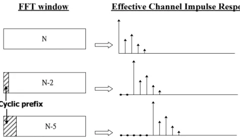
Fig 2.10 Effective channel impulse response due to inaccurate FFT window

As Fig 2.10 is depicted, the symbol timing offset in ISI-free region causes path time delay of effective channel impulse response. We assume that the signal is transmitted over multipath fading channel characterized by

1 0 ( , ) L l( ) ( l) l hτ t − h t δ τ τ = = ⋅ − (2.20)

where h_l(t) are the path complex gains, τ_l are the path time delay, and L is the total

number of paths. Then the effective channel model due to symbol timing offset changes to be

1 0

( , ) _lL _l( ) ( _l )

hτ t = ₌− h t ⋅δ τ τ ε− + ⋅ T (2.21) Therefore, the fine symbol timing can be maintained by acquiring the effective channel impulse response (CIR) and then estimating the main path delay. The path delay estimation task utilizes the channel frequency response (CFR) estimated by channel estimation unit and subsequently performs an IFFT to transform the CFR to CIR.

Before detail discussion of path time delay in CIR estimation, channel estimation should be introduced in advance. In channel estimation design, 2-D interpolation is generally used because of its robustness for mobile time-variant channel caused by Doppler spread. In 2D interpolation, channel gain estimations at scattered pilots are first interpolated over

(32)

interpolation is adopted in two adjacent symbols with same scattered pilot modes for

estimating the channel gain of scattered pilot within the interval. Afterward, all other channel responses are obtained by frequency-dimension interpolation. This 2-D interpolation method deserves to be applied in DVB-T system even though large memory requirement. The time-dimension interpolation can overcome the severe time-variant channel and channel frequency response can be estimated effectively.

After time-dimension interpolation, a total of Kmax/3+1 sub-sampled channel gain of

scattered pilots are available. To provide a sufficiently accurate estimation, a zero padded IFFT of size N/2 must be used. The operations of fine symbol synchronization are illustrated in Fig 2.11. N FFT N FFT N/2 IFFT N/2 IFFT Zero Padding Zero Padding ROM Pilot ROM Pilot Scattered Pilot Extraction Scattered Pilot Extraction FFT Window FFT Window Peak Decision Peak Decision Time-dimension interpolation Time-dimension

interpolation Frequency-dimensionFrequency-dimensioninterpolation_{interpolation}

Fig 2.11 Structure of fine symbol synchronization

Fig 2.11 shows the process of fine symbol synchronization including zero padding, N/2

IFFT and peak decision. The fine symbol synchronization utilizes the CFR of Kmax/3+1

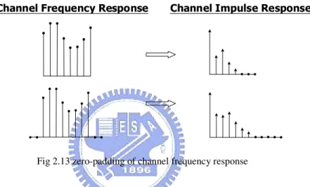
scattered samples after the time-dimension interpolation and then performs zero padding to size N/2. The changes of spectrum due to downsampling and zero padding are drawn in Fig 2.12 and Fig 2.13 respectively.

(33)

Fig 2.12 Downsampling of channel frequency response

Fig 2.13 zero-padding of channel frequency response

Fig 2.12 shows a basic concept of downsampling in frequency domain. The resulting time domain response after sampling in frequency domain is CIR duplication. Then downsampling causes CIR expansion so that the original CIR can be computed with a little aliasing. It has been known that low pass filtering has to be done prior to downsampling for avoiding aliasing. However, the effect of aliasing is slight because the power of CIR usually centralizes in the prior paths and hence the low pass filtering can be neglected if the downsampling rate is not too large.

Fig 2.13 illustrates the effect of zero-padding. We can assume the zero padding in frequency domain as the spectrum compression and hence CIR expands according to the ratio of compression in spectrum. In our design, the channel gain of subcarrier is zero-padded from N/3+1 to N/2. In terms of spectrum, we can regard as spectrum compression with a ratio of

(34)

2/3 and thus CIR will expand with a ratio of 3/2. Therefore, the resolution of estimated CIR is 2/3. The resulting sampling resolution is

' 2 / 3 3 _est N T T T N = = (2.22)

In order to promote the peak detection, the square operation is performed with the resulting estimated CIR. After the square operation, the difference between channel impulses will be more apparent and hence the probability of wrong peak detection can be reduced. As a result, the expression of peak detection can be represented as

^ ₂ k _k S = h (2.23) ^ ₂ ^ arg max( ) 3 k Sk δ = (2.24)

It’s obvious that the fine symbol synchronization with N/2 IFFT method dominates the complexity of overall synchronization system. Therefore, we proposed a low complexity solution of fine symbol synchronization. The size of IFFT can be reduced by downsampling the estimated channel frequency response. However, the aliasing will occur if the downsampling rate is too large. In order to eliminate aliasing, we apply a 16-point average window as lowpass filter in advance. We then downsample the CFR by 16 so that the complexity can be reduced substantially. The proposed low complexity fine symbol synchronization design is depicted as Fig 2.14. The simulation results will be shown in Chapter 3. N/32 IFFT N/32 IFFT _Zero Padding Zero Padding Peak Decision Peak Decision ! "# Average Window Average Window 16 16 "

(35)

2.3 Sampling Clock Synchronization

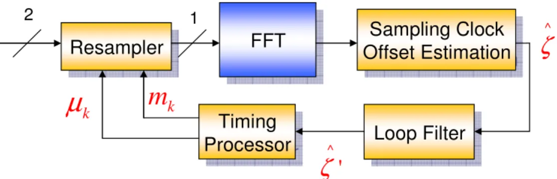
The purpose of the sampling clock synchronization is to alter the sampling frequency and sampling phase. If the sampling timing recovery is properly operating, it will provide the downstream processing blocks with the samples at the highest SNR available. The proposed sampling clock synchronization is an all-digital timing recovery loop which is shown in Fig 2.15. After ADC conversion, the oversampled signal is passed through a resampler which consists of an interpolator and a decimator. The interpolator is able to generate samples within those actually sampled by ADC. By generating these intermediate samples, the interpolator can adjust the sampling timing as needed. The purpose of decimator is to get different sampling rate of received data. In our receiver design, the decimator downsamples the received signals from twofold-oversampling to original sampling rate.

The information of timing error is computed by sampling clock offset estimator. The sampling clock offset estimator can use a number of different algorithms to generate a detected sampling clock offset. The control signal of resampler is formed by filtering the

estimated SCO, i.e., denoted by ζ^ , using an PI loop filter. Timing processor receives the

filtered SCO ζ^' and computes the corresponding parameters required by resampler,

basepoint m and fractional timing offset _k µ_k.

k

µ

Resampler

FFT

_{Offset Estimation}

Sampling Clock

_{Offset Estimation}

Sampling Clock

Timing

Processor

Timing

Processor

Loop Filter

2 ₁ k

m

^

ζ

^

'

ζ

(36)

2.3.1 Sampling Clock Offset Estimation

As previous mentioned, the effect of sampling clock offset in frequency domain is phase rotation which increases every symbol. Referring to Eq(2.12), the difference of phase rotation between two consecutive symbols can be represented as

1 '( ) ( ) ( ) 2 2 l l l s s k k k N k fN T N ϕ ϕ ϕ π ζ π − = − ≈ ∆ + (2.25)

where f∆ is residual carrier frequency offset, ζ is sampling clock offset, Ns is OFDM

symbol length equal to N + Ng and k denotes the subcarrier index, −K/2≤k≤K/2−1.

We can assume carrier frequency offset f∆ causes mean phase error and sampling

clock offset ζ causes linear phase error between two consecutive symbols. If we take two

adjacent continual pilots of arbitrary two consecutively received OFDM symbols, the phase rotation is shown in Fig 2.16. The total phase rotation includes the effects of symbol timing offset, CFO and sampling clock offset. In the previous symbol, the magnitude of phase rotation due to symbol timing offset is proportional to subcarrier index. In the current symbol, the effect of CFO and sampling clock offset are accumulated in the phase of previous symbol, where the sampling clock offset induces linear phase and CFO generates mean phase. Thus, we have to estimate the sampling clock offset as well as residual CFO by computing the phase rotation between two consecutive symbols.

(37)

Adjacent Continual Pilot Symbol timing offset CFO Sampling clock offset $ %

Fig 2.16 Phase rotation between two consecutive symbols

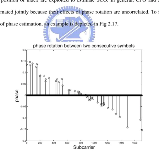
Since the phase rotation is proportional to subcarrier index, the continual pilots which have fixed position of index are exploited to estimate SCO. In general, CFO and SCO are usually estimated jointly because their effects of phase rotation are uncorrelated. To illustrate the subject of phase estimation, an example is depicted in Fig 2.17.

0 200 400 600 800 1000 1200 1400 1600 -0.2 -0.15 -0.1 -0.05 0 0.05 0.1 0.15

0.2 phase rotation between two consecutive symbols

Subcarrier

ph

as

e

Fig 2.17 Phase error between two consecutive symbols

(38)

Because of the distortions caused by AWGN, residual ICI and time-variant multipath fading channel, the effect of phase rotation is not as perfect as theoretical value. Therefore, the task of SCO estimation is to find the total phase rotation over the whole OFDM symbol spectrum for averaging the estimation noise. In reference [3], a joint SCO and CFO tracking algorithm is proposed shown as ^ 2, 1, 1 1 ₍ ₎ 2 (1 g/ ) 2 l l f N N ϕ ϕ π ∆ = ⋅ ⋅ + + (2.26) (1|2) ^ * 2, 1, 1|2, , 1, 1 1 ( ) arg 2 (1 / ) / 2 l l l l k l k k C g z z N N M ζ ϕ ϕ ϕ π − ∈ = ⋅ ⋅ − = ⋅ + (2.27)

where l denotes symbol length, k denotes subcarrier index and zl,k represents subcarrier after

FFT operation. Let C1 denotes the set of continual pilots which index in the left half

) 0 , 2 / ) 1 ( [− − ∈ M

k and C2 the set of continual pilots which index in the right half

] 2 / ) 1 ( , 0 ( − ∈ M

k of the OFDM symbol spectrum. Applying correlation of continual pilots in

two consecutive symbols and accumulation of the correlation results in two parts lead to the so-called CFD/SFD (carrier frequency detector / sampling frequency detector) algorithm. The

summation of ϕ₂_l, and ϕ₁_l, can compute mean phase error while the subtraction of ϕ₂_l,

and ϕ₁_l, produces the linear phase. As a result, SCO and CFO can be estimated jointly by

multiplying different constants. However, this algorithm to divide continual pilots into left and right parts and then to accumulate the correlation results is suitable only in the equally distributed pilots. In DVB-T system, the distribution of continual pilots is not exactly equal as shown in Fig 2.17, so that this jointly CFD/SFD algorithm will always generate an unavoidable error in the SCO estimation. In order to improve this problem, a new SCO estimation algorithm is proposed.

As previous mentioned, the purpose of SCO estimation is to compute the phase rotation over the whole OFDM spectrum. Therefore, the subject can be simplified to find the slope of the linear regression line as shown in Fig 2.18 and hence we introduce the linear least square

(39)

regression calculator to estimate it. In order to illustrate the linear least square (LLS) method,

we assume the candidate regression line is y= f(x;a₀,a₁)=a₀+a₁x. The process of LLS

regression is to minimize the summation of square errors such as

2 2 0 1 1 1 [ ( )] [ ( )] K K i i i i i i E y f x y a a x = = = − = − + (2.28)

Then we have to compute the gradients of

0 a E ∂ ∂ _and 1 a E ∂

∂ _{. After letting the gradients be zero,}

a0 and a1 can be computed as optimal value.

0 200 400 600 800 1000 1200 1400 1600 -0.2 -0.15 -0.1 -0.05 0 0.05 0.1 0.15

0.2 Linear least square regression line

Subcarrier

ph

as

e

Fig 2.18 Linear least square line

In fact, we can also suppose each xi passes through this candidate line such as

K K y x a a y x a a y x a a = + = + = + 1 0 2 2 1 0 1 1 1 0

(40)

y

A

y

x

K K

θ

=

2 1 2 1 2 1

1

We have to evaluate θ in terms of minimizing square error E

2

( ) (T )

E= −y Aθ = y A− θ y A− θ (2.29)

As a result, the theoretical value of θ can be computed by

1

(_{A A A y}T ) T

θ ₌ − _(2.30)

The slope θ2 is linear phase error and thus can be applied in SCO estimation. On the other

hand, the resulting shift θ1 can be regarded as mean phase error so that the CFO estimation

can be also done in linear least square regression method. This joint SCO/CFO estimation method can replace the CFD/SFD algorithm for avoiding the error caused by unequally distributed continual pilots. The LLS algorithm can be sown as

/ 2 1 ^ 1, , / 2 1 2 (1 / ) M k l k k M g f B y N N π − =− ∆ = ⋅ ⋅ + (2.31) / 2 1 ^ * 2, , , , 1, / 2 1 1 2 1 arg 2 (1 / ) ( ) 1 1 | 1 M k l k l k l k l k k M g T T M B y y z z N N B A A A k k A k CP k ζ π − − =− − = ⋅ ⋅ = ⋅ + = = ∈ (2.32)

where B1,k represents the first row of matrix B and B2,k the second row. k denotes the

subcarrier index of continual pilot.

In DVB-T system, A represents the distributed indexes of continual pilots, which has been known before receiving signals. Therefore, the complicated matrix operation

T

T_A _A

A ₎ 1

(41)

are left to several multiplications and accumulations. The complexity is almost the same as CFD/SFD algorithm [3]. The performance improvement will be discussed in Chapter 3.

2.3.2 Resampler

The resampler consists of interpolator and decimator. The task of interpolation is to compute intermediate values between signal samples and decimation executes the downsample process which makes the 2-times oversampling signals received from ADC become signals with original sampling rate. In fact, the decimation process can be accomplished by the interpolation filter itself and hence the separate decimator is not required.

It has been well know that the band-limited input signal x(t) or its samples {x(kTi)} at

time t=kTi ) could be recovered by using the ideal filter with sinc function which has

frequency response sin / ( ) / s I s t T h t t T π π = (2.33)

and impulse response

1 , | | ( ) 2 0, s s I T f T H f otherwise < = (2.34)

We assume the symbol timing t= kT+τ as (mk +µ)Ts, where τ is the timing offset,

k

m is an integer and 0<µ<1. Subsequently, we can estimate x(kT+τ) by interpolation:

[( _k ) ]_s [( _k ) ] ( )_s _n ( ..., 1, 0,1, ...)

n

y m µ T ∞ x m n T h µ n

=−∞

+ = − = − (2.35)

where hn(µ) is the interpolation filter for fractional timing µ

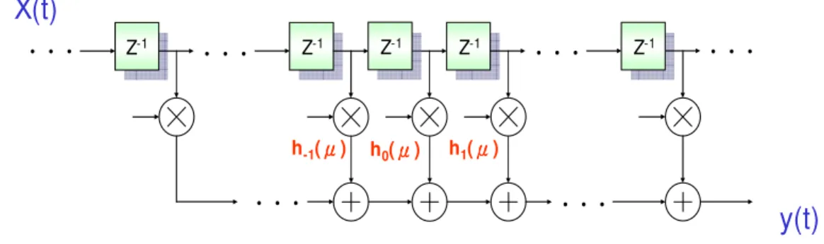
( ) ( , ) sin ( ) / ₍ _{..., 1, 0,1, ...)} ( ) / n I s s s s s s s s h h nT T nT T T _n nT T T µ µ π µ π µ = + = = − + (2.36) Conceptually, the ideal filter can be thought of as an FIR filter with an infinite number of taps.

(42)

The coefficient of taps are a function of µ. The structure of the sinc interpolation filter is shown in Fig 2.19. Z-1 Z-1 Z-1 Z-1 Z-1 Z-1 Z-1 Z-1 Z-1 Z-1 h0( ) h-1( ) h1( )

X(t)

y(t)

Fig 2.19 Ideal interpolator

The corresponding impulse response of hn(µ) is illustrated in Fig Fig 2.20. Fig 2.20 shows

the coefficient of each tap in the sinc interpolation filter.

) (µ n h 0 = µ (a) h_n( )µ , µ= 0

(43)

) (µ n h 2 . 0 = µ (b) h_n( )µ , µ=0.2

Fig 2.20 Coefficients of h_n( )µ using sinc function

Theoretically, perfect signal recovery can be achieved by an ideal filter with infinite taps. However, for a practical receiver design the interpolator must be approximated by a finite-order FIR filter

2 1 [( _k ) ]_s I [( _k ) ] ( )_s _n n I y m µ T x m n T h µ =− + = − (2.37)

The filter performs a linear combination of the (I1+I2+1) signal samples x(nTs) taken

around the basepoint m . The truncated coefficients of the outside taps raise the side-lobe _k

amplitude of frequency response. It is necessary in practice to window the ideal impulse response instead of removing the tail coefficients simply so as to make it finite.

There is a tradeoff between the main-lobe and side-lobe area when we are seeking the window function. The issue was considered in depth in a series of classic papers. The solution found previously are difficult to compute and therefore unattractive for filter design. However, Kaiser (1966, 1974) found that a near-optimal window could be formed using the zeroth-order modified Bessel function of the first kind, which is much easier to compute. The Kaiser window is defined as

(44)

2 1/ 2 0 0 [ (1 [( ) / ] ) ] , 0 , [ ] ( ) 0, , I n n M w n I otherwise β α α β − − _{≤ ≤} = (2.38)

where α=M/2 and I₀(⋅) represents the zeroth-order modified Bessel function of the first

kind which is defined by

2 0 0 ( / 4) ( ) ! ( 1) k k z I z k k ∞ = = Γ + (2.39)

where Γ is a gamma function. (⋅)

The Kaiser has two parameters: the length (M+1) and a shape parameter β. The

window length and shape can be adjusted to trade side-lobe amplitude for main-lobe width.

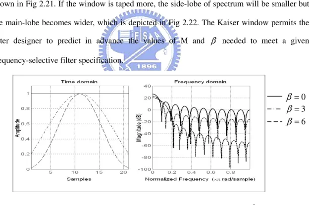
The frequency response of the Kaiser window with M=20 and different parameter of β is

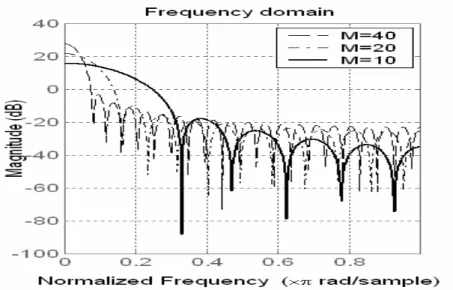
shown in Fig 2.21. If the window is taped more, the side-lobe of spectrum will be smaller but the main-lobe becomes wider, which is depicted in Fig 2.22. The Kaiser window permits the

filter designer to predict in advance the values of M and β needed to meet a given

frequency-selective filter specification.

3 =

β

6 =

β

0 =

β

(45)

Fig 2.22 Frequency response of Kaiser window with different taps of M

In order to obtain better performance of interpolation, the sinc function truncated by a

Kaiser window is used in interpolation filter design. The resulting function hn(µ) is defined

as 2 1/ 2 0 0 sin ( ) / [ (1 [ / ] ) ] ( ) 1 ( ) / ( ) 2 2 s s s n s s s nT T T I n M M h n nT T T I π µ β α µ π µ β + − = ⋅ − ≤ ≤ − + (2.40)

where α=M/2. The frequency response of 61 taps sinc function which can be regarded as

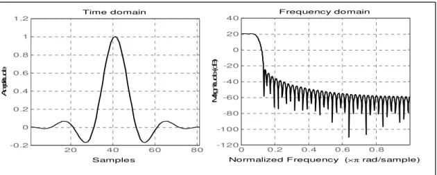
infinite approximately is depicted as Fig 2.23(a). If we truncate sinc function at the third zero crossing to the left and right of the origin, we obtain the frequency response shown in Fig 2.23(b). Note that the relative side-lobe attenuation enhances to 1.3db from 0.2db and the start of stopband raises from -20db to 0db. Fig 2.23(c) shows the frequency response of the sinc function truncated with a Kaiser window. Obviously, its side-lobe becomes slow and relative side-lobe attenuation is reduced so that the performance is improved. The relative simulation performance will be mentioned in Chapter 3.

(46)

200 400 600 -0.4 -0.2 0 0.2 0.4 0.6 0.8 1 Samples A m pl itu de Time domain 0 0.2 0.4 0.6 0.8 -120 -100 -80 -60 -40 -20 0 20 40

Normalized Frequency (×π rad/sample)

M ag ni tu de (d B ) Frequency domain

(a) Frequency response of 61-tap sinc function

(Relative side-lobe attenuation: 0.2db, Main-lobe width: 0.19849)

20 40 60 80 -0.4 -0.2 0 0.2 0.4 0.6 0.8 1 Samples A m pl itu de Time domain 0 0.2 0.4 0.6 0.8 -100 -80 -60 -40 -20 0 20 40

(b) Frequency response of 9-tap sinc function

(47)

20 40 60 80 -0.2 0 0.2 0.4 0.6 0.8 1 1.2 Samples A m pl itu de Time domain 0 0.2 0.4 0.6 0.8 -120 -100 -80 -60 -40 -20 0 20 40

(c) Frequency response of 9-tap sinc function truncated by Kaiser window (Relative side-lobe attenuation: 0.1db, Main-lobe width: 0.18164)

Fig 2.23 Frequency response of 61-tap sinc function, 9-tap sinc function and sinc function truncated by Kaiser window

2.3.3 Timing Processor

This section focuses on the control of the resampler. In SCO tracking loop, sampling clock offset will be computed every two OFDM symbols. The task of timing processor is to

determine the basepoint m and the corresponding fractional delay _k µ_k as the time-variant

coefficients based on the output of sampling clock offset estimator. The basic concept of interpolator control has been already described in [12]. In this section, the simpler and clearer structure will be illustrated for hardware consideration.

To recovery the sampling timing, it has to compute the corresponding basepoint m and _k

the fractional delay µ_k every sample based on the loop-filtered SCO 'ζ . The relation

between the received samples, transmitted samples, m and _k µ_k is illustrated in Fig 2.24.

Fig 2.24(a) illustrates the condition of SCO = 0.4 while Fig 2.24(b) shows the condition of

SCO = -0.3. Note the basepoint m not really represents the index of basepoint and it _k

(48)

operates normally with the following sample as basepoint. The case of m_k = 1 represents that current received sample must be discarded and basepoint is replaced by next sample as

shown in Fig 2.24(a). Note that the fractional delay µ_k is defined in the interval of [0, 1).

For the hardware consideration, it means that the FIR filter should bypass a sample when the

computed m_k = 1. Contrary to the condition of positive SCO as Fig 2.24(a), negative SCO

causes that the basepoint must apply the same sample twice, which is denoted by m = -1 as _k

shown in Fig 2.24(b). The repeated samples imply that a lot of buffers will be needed. This is not desirable in the practical filter design. Fortunately, this problem can be easily solved by merging decimation process with the interpolator. The subject will be discussed in the later section. k k m µ 4 . 0 = ζ (a) SCO = 0.4 k k m µ 3 . 0 − = ζ (b) SCO = -0.3

(49)

For a given ζ , it is easy to find out the relation between m_k, µ_k and ζ . The

sampling timing varies with the SCO ζ . Taking Fig 2.24(a) for example, the first received

sample from original synchronized sample has a timing offset of 0.4 comparing with transmitted first sample. In the second sample, the difference of sampling timing between received data and transmitted data becomes 0.8, double of 0.4. Similarly, the third sample should get the offset value of 1.2 which implies the sampling timing offset exceeds one

sample. Since we define 0≤µk <1, we should take the fractional part of µk, 0.2, and the

integer part becomes m so as to apply the next sample as basepoint. The recursive _k

estimation is represented by 1 1 ' ' k k k k k m m µ ζ µ µ ζ − − = + = + − (2.41)

where ζ is replaced by 'ζ since the timing processor actually receives the loop-filtered

SCO 'ζ rather than SCO ζ .

In order to illustrate the decimation process merging within interpolator, we take an

example as Fig 2.25. There are two exaggerated cases of different 'ζ listed in Fig 2.25. Left

case describes the behavior of timing processor in the condition of positive 'ζ =0.6 and initial

timing offset µ₀=0. Right case also shows the computation of corresponding m and _k µ_k

in the condition of negative 'ζ =-0.2 and µ₀=0.3. The calculations of m and _k µ_k are

應用於地面數位電視廣播系統之時序同步化設計

Timing Synchronization for DVB-T System

Student : Cheng-Wei Kuang Advisor : Dr. Chen-Yi Lee

Institute of Electronics Engineering

National Chiao Tung University

ABSTRACT

Contents

List of Tables

List of Figures

Chapter 1

Introduction

1.1 Motivation

1.2 Introduction to ETSI DVB-T Standard

1.3 Thesis Organization

Chapter 2

Timing Synchronization Algorithms

2.1 Introduction to Timing Offset

2.1.1 Effect of Symbol Timing Offset

ε

2.1.2 Effect of Sampling Clock Offset

α

α

2.2 Symbol Synchronization

2.2.1 Mode / GI Detection

2.2.2 Coarse Symbol Synchronization

(

)

(

)

2.2.3 Scattered Pilot Mode Detection

2.2.4 Fine Symbol Synchronization

2.3 Sampling Clock Synchronization

µ

Resampler

Resampler

FFT

FFT

Offset Estimation

Sampling Clock

Offset Estimation

Sampling Clock

Timing

Processor

Timing

Processor

Loop Filter

Loop Filter

m

ζ

'

ζ

2.3.1 Sampling Clock Offset Estimation

y

A

y

y

y

x

x

x

θ

θ

θ

=

1

1

1

2.3.2 Resampler

X(t)

y(t)

β

β

β

2.3.3 Timing Processor

_{Offset Estimation}

_{Offset Estimation}