Modeling and performance evaluation for automated material handling systems in a 300 mm foundry fab

Proceedings of the 2002 IEEE International Conference on Robotics & Automation

Washington, DC May 2002

Modeling and Performance Evaluation for Automated Material Handling Systems in a 300"

Foundry Fab

Han-Pang Huang*, Chun-Tsong W a g *

*

Robotics Laboratory, Department of Mechanical Engineering National Taiwan University, Taipei, 10674 Taiwan Email: hanpana@ccms.ntu.edu.tw TELEAX: (+886-2) 2363-3875

*

Abstract

In this paper, a modeling methodology for conceptual design of automated material handling system using distributed colored timed Petri net (DCTPN) will be developed. The IC fabrication process-flow model is constructed and integrated with AMHS models. Especially, in IC fabrication process-flow modeling, a method called virtual tool group will be proposed to solve the problem in modeling tool-coupling effects. From this entire fab model, several performance indexes, such as WIP, bottleneck detection, cycle time, wafer operation history tracking, and vehicle utilization can be evaluated from DCTPN simulation result.

1.

Introduction

Internationally, all the super power of semiconductor factory is dedicated to develop the 300 mm IC foundry fab. Since it is expensive to introduce a fab-wide automation, it is important to evaluate the entire system and make a suitable design in early stage of planning. The system configuration is also an important subject since it affects the system eEcient a lot. Hence, the DCTPN model of

AMHS that utilizes the transport, hoisting, pushing vehicle, finding nearest vehicle, intelligent control and zone control will be constructed. In addition, DCTPN model of AMHS will be integrated into the fab model that was constructed by Kuo [6]. The entire fab DCTPN model after integrating can act as a virtual fab, and can be used to estimate fab and AMHS performance and behavior more correctly.

Petri net is highly effective for modeling, simulation, and scheduling discrete event systems. It is also usefbl for designing and implementing controllers for manufacturing [12]. Some researches have focused on performance evaluation through Petri nets [4] [5] [6] [12]. The 200 mm and 300 mm fabs will place stringent requirements on their automated material handling systems (AMHS). There are several researches on AMHS for 300 mm IC foundry fab. [3] [7] focused on the practicality of AMHS in a 300 mm fab, and the advantages of automation were also validated. Chen [l] emphasized the study on dispatching rules. The dispatching rule plays a very important role in a material handling system and takes significant effects on system performance.

Egbelu and Tanchoco [2] divided the vehicle dispatching decisions into two categories: workcentre initiated task assignment problem and vehicle initiated task assignment problem. When there is only one vehicle in the

system, collision, blocking and deadlocking can never happen. The system needs no traffic control. The system can run as long as the vehicle can move. When there is more than one vehicle in the system, traffic problem may occur and the traffic control is necessary.

2. Model Architecture of IC Foundry Fab

Since the behaviors and activities in an IC foundry fab are complicated, it is necessary to use a systematic modeling method to deal with such a complex system. Since the DCTPN [ 5 ] is a modular design, the system can be divided into several modules. Each module can communicate with each other through NTU Net. Based on this modeling concept, a complete manufacturing system can be modeled by distributed, modular and flexible configurations. Hence, DCTPN is a good tool for modeling the IC foundry fab.

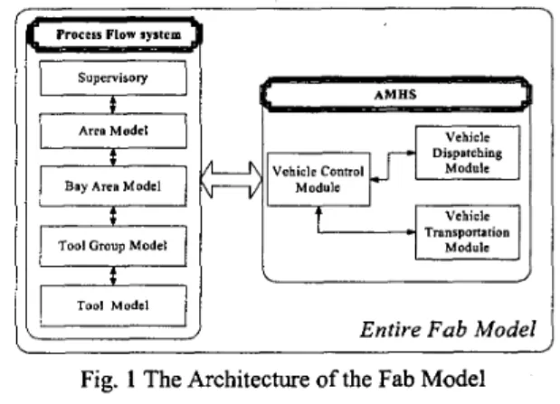
The architecture of entire fab model is shown as Fig. 1. There are two sub-systems: process flow system and AMHS. Each sub-system is composed of several sub-nets or modules.

Supervisory

Area Model

Tool Group Model

Tool Model

Entire Fab Model

I

Fig. 1 The Architecture of the Fab Model

3.

Process Flow Model

In a traditional IC fab, the area and tool group architectures are commonly used. A fab is configured in terms of the plant, areas, tool groups and tools hierarchically. Thus, the process flow model is constructed based on the hierarchy. Clearly, the hierarchical configuration and modular modeling methodology makes the modeling work become more flexible and extensible.

Although the hierarchical configuration of the IC fab makes the modeling of an IC foundry fab become straightforward. However, in this configuration, each tool is forced to be included in one tool group only. That is, the

coupling effect [23] between tools and tool groups are not considered in this model. The reliability of the model is decreased due to differences between the fab model and the real fab, especially in the capacity of the tool groups. The concept of “Virtual Tool Group” enables the DCTPN to model the coupling effect easily. Table 1 shows the relation between tools and tool groups.

Tool Group $G1

$G2

Table 2 Relation Table between Tool Group and Virtual Tool Grour,

Virtual Tool Group $VTG2

1

I

WTG2

I

$G6 $VTG 1

Table 3 Relation Table between Virtual Tool Group and Tools

I

I

1

The central concept of the virtual tool group is “Each tool is included in only one virtual tool group; a tool group may be composed of several virtual tool groups.” It is a logical layer between tool groups and tools. Based on this central concept, the algorithm of virtual tool group is summarized as the following four steps:

Build the relation table between tool groups and tools Search for the tool, which is included in only one tool group. Select these tools and the tool groups contained those tools. Check each selected tool group. For each selected tool group, build a new virtual tool group to include these tools.

Check many to many relations for the rest tools after stepl. In this step, search for the tool, which is included in more than one tool groups. Select the tool groups that contain these selected tools. Build new virtual tool groups that contain the tools belonging to more than one tool group.

Repeat steps 2 and 3, until each tool is included in only one virtual tool group.

The result shows in Table 2 and Table 3.

4.

AMHSModel

In a 300 mm foundry fab, all transportation works are done by AGVs. Hence, the dispatching rules and traffic control of AGVs must be considered to maximize performance.

4.1.

4.1.1. Collision free

Traffic Control of the AMHS model

Zona 2 Zon. 3

P-01 T-01 P 03 T-02 P-04 T-03 P-06

I

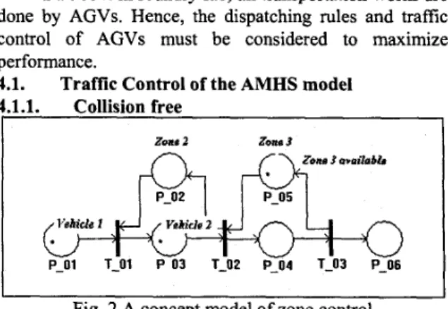
Fig. 2 A concept model of zone control

A zone control strategy is often used for collision free purpose. In zone control, a traveling vehicle will stop whenever another vehicle is detected in the zone ahead. Fig. 2 shows a conceptual model of zone control. In this model, tokens in P-01, P-03 and P-04 describe vehicle at zone 1, zone 2 and zone3, respectively. Tokens in P-02 and P 05 denote zone 2 and zone 3 available.

Fig. 3 A concept model of Push Vehicle with Zone Contrc 4.1.2. Blockage phenomenon

Blockage occurs while idle vehicles occupy the zones of the path that another vehicle will go through. An intelligent control system should actively push the idle vehicles away to keep the guide path available for the loaded vehicle [l]. The DCTPN model of push vehicle is shown as Fig. 3. In this model, P-07 is a resource place of

idle vehicles. Here, if vehicle 1 cannot enter zone 2, then vehicle 1 should check whether another idle vehicle occupies zone 2 from P-07. If “Yes”, then the event of “Push Vehicle” is fired and the movement command of “from zone 2 to zone 3” is given by T-04. Otherwise, the event of “Wait” is fired. When the vehicle travels form zone 2 to zone 3, T-02 must be fired and zone 2 becomes available again. Hence, vehicle 1 can enter zone 2. The timed transitions T-01 and T O 2 denote the transportation times between each zone.

4.1.3. Deadlock Phenomenon

The deadlock phenomenon is a conflict condition between a tool and vehicles. A feasible solution for such situation is that the loaded vehicle sends the lot to the stocker for temporary inventory until the tool become available. Fig. 4 demonstrates the model of “Send To Stocker”. In this model, P-02 denotes a temporary inventory that stores the lots waiting for tool 1 or tool2. P-07 and P-08 describe whether Tool 1 and Tool 2 is available. If P-07 has one token, then tool 1 is available. Note that T-02 can be fved only when tool 1 is available. It means the lot can be processed on tool 1 while tool 1 is available. Thus, deadlock situation will never happen in such model. In addition, macro transition T-04 and T-32 describe intrabay AMHS. After the lot is assigned to be processed on tool 1, the lot is sent fi-om stocker to tool 1 by intrabay AMHS through T-04. While the process of the lot is finished, the lot is sent from tool 1 to the stocker from intrabay A M H S through T-32. Therefore, the tool is available again while the vehicle moves the lot to the stocker.

.

x

Fig. 4 Demonstration of “Send To Stocker” 4.2.

There are three steps for the dispatching configuration in this paper: equipment-based, workcentre initiated task assignment and vehicle initiated task assignment. In “Equipment-Base Selection”, the equipment selects the lot that waiting for manufactured. The second stage is workcentre initiated task assignment. Here, the NV (Nearest Vehicle) is always selected in this paper because of its superior performance over the other rules in published research [2]. The third stage is vehicle initiated task assignment. Several researches indicated that minimize the AGV travel distance might have a better performance[8]. Hence, the dispatching rule of STTD (Shortest Traveling TimeDistance) is selected.

4.2.1. DCTPN model of Control Strategy 1

In this control strategy, the vehicle initiated work center selection can be selected in transition T-02. The selection set of the dispatching including FCFS and ERT. The workcentre initiated work center selection uses NV (Work search for nearest vehicle). The model of this

Dispatching Module of AMHS Model

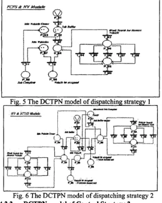
strategy is shown in Fig. 5 . In this model, all movement requests will be sent to P-02 through communication place P-01. The tokens in P-03 indicate the numbers of idle vehicles. When a movement command arrives and there are more than one idle vehicles, T-02 will be fired. P-04 is a conflict place. The conflict resolution used here is priority. First, check whether T-10 can be fired. If not, then fire T-03. The input criterion of T-IO is attribute match. If the start point of the lot is the same as the idle point of the vehicle, then T-IO will be fired. This means the vehicle can serve the lot right away without any transportation. If T-10 cannot be fired, it means the start point of the lot is different from the idle point of the vehicle. If T-IO cannot be fired, it means no idle vehicle is on the start point of the lot. Hence, the lot must search for a nearest vehicle for transportation.

r

I

Fig. 5 The DCTPN model of dispatching strategy 1

Fig. 6 The DCTPN model of dispatching strategy 2 4.2.2.

In this strategy, the vehicle initiated dispatching rule is STT/D. The workcentre initiated dispatching rule is Nv. The model dispatching control strategy is shown in Fig. 6 . In this figure, vehicle will check whether another transportation job needs to be severed after finishing a job (T-04). If yes, T-04 will be fired and the vehicle will search for a nearest lot from job buffers to serve. If no, T-20 will be fired and the vehicle becomes idle and waits for the next job at P-05.

4.3.

Each AMHS model is composed of

A M H S

DCTPN model of Control Strategy 2

into A M H S control net and AMHS movement net. The main responsibility of AMHS control net includes vehicle path control, vehicle dispatching and communicate with process flow net. On the other hand, the main responsibility of AMHS movement net includes vehicle traffic control, and vehicle transportation time between each stop point.

5.

Simulation and Performance Analysis

In this section, a real world IC wafer fabrication system (Hewlett-Packard Technology Research Center Silicon fab, hereafter called TRC fab) is used as the target plant for implementation. Wein [ 101 constructed the TRC fab model in 1988. In addition, he used a variety of input controls and lot sequencing rules to evaluate the performance by simulation. In order to justify the proposed model, the constructed fab model will be compared to Wein’s model and are discussed in section 0, several dispatching control strategies are compared by simulation and discussed in section 5.2.

model Sim.1 Sim.2 5.1. Model Verification nit: Hour Mean Total Queuing Time 1208 1059 998 In order to make precise comparison, the configurations of simulations are the same as Wein’s model [ 101. Considering the warm-up period of the system, the simulation data is collected from a period of 10000

hours to 20000 hours. The model comparison between Wein’s and this study is shown as Table 4. From the simulation result, the operation time of Wein’s model, Siml and Sim2 are close. Hence, the correctness of the proposed model can be justified. On the other hand, the total queuing time of Siml and Sim2 are less than Wein’s result. This difference comes from the effects of

considering the machine failures in Wein’s model. Because the machine failure will decrease manufacturing capacity, each lot has to spend more time waiting for available machines. Hence, the mean queuing time is larger in Wein’s model. In addition, from the comparison of Sim.1 and Sim.2, lot-sequencing rule using ERT is better than using FCFS. This is because the reentrant flow and high WIP level characteristics in semiconductor manufacturing. If lot sequence rule is FCFS, each reentrant lot to a certain buffer has to wait until the other waiting lots have been manufactu5ed no matter how emergency the reentrant lot is. However, since high WIP level manufacturing characteristic, each reentrant lot has to wait for a quite

long time until begins to operate. Hence, the queuing time of Sim. 1 is larger than Sim.2.

5.2. Performance Evaluation

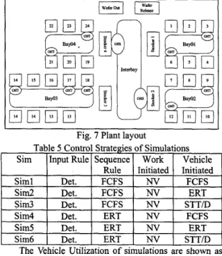
In this section, TRC fab model with AMHS will be considered by simulation. The entire TRC fab layout with AMSH is assumed as Fig. 7. In addition, in order to increase the utilization of vehicles and tools, the internal buffer of each tool is set as 2. The control strategies of simulations are listed in Table 5. Considering the warm-up period of the system, the result of simulation data is

dlected from a period of 10000 hours to 20000 hours.

P

I

E]

Fig. 7 Plant layout

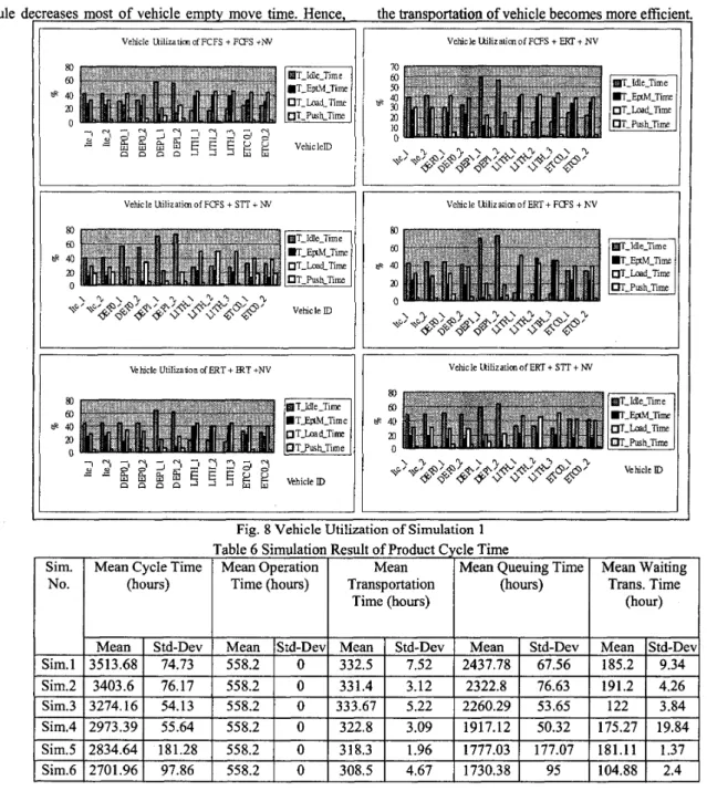
The Vehicle Utilization of simulations are shown as Fig. 8 and. From the results, the load vehicle utilization in LITH-1, LITH-2, LITH-3, ETCO-1, and ETCO-2 (bay03, bay04) are higher than the others. Production route and equipment layout can be used to explain this situation. Note that this simulation uses single production route, and most operations of the route are at bay03 and bay04 (351172 in bay01, 121172 in bay02, 651172 in bay03 and 601172 in bay04). On the other hand, the bay length of bay03 is higher than others. It may also cause high load vehicle utilization in bay03. The send-to-stocker control ,

strategy also increases the transportation jobs. In addition, the empty move time of vehicles is almost 60% more than load move time except in Sim.3 and Sim6, especially in Bay03 and Bay04. That means a vehicle is always moving a quite long distance to take the lot after it is assigned. This may decrease the performance of the AMHS. In simulation 3 and simulation 6, the vehicle initiated dispatching rule is changed to STT. That is, vehicle will search for the nearest job to serve while completing a transportation job. By simulation result, this dispatching

rule c xeases most of vehicle empty move time. Hence, the transportation of vehicle becomes more eficien Vehicle Uiliraticn of FCFS + FCFS +Nv

I

~~

Vehicle Urilizaiim of FCFS + STT + W

I

Vehicle Uilizatim of F P S + ERT + NV

I

Vehicle Urilizatim of ERT t FCFS + NV

I

Vehicle Uilizaticm of ERT + SlT + NV

Fig. 8 Vehicle Utilization of Simulation 1

5.2.1. Product cycle time Analysis

The product cycle time (including process time, traveling time and waiting time) is defined as the time

from wafer release to completion. The simulation result between time duration 10000 hours and 20000 hours is shown in Table 6 . One should mention that the transportation time of each simulation case is different. This is due to occurrence of the push vehicles. In addition, the control strategy of Sim.1 is the same as Wein’s model

that was discussed in section 0. However, the queuing time

is much larger than Wein’s simulation result. This is because the effects of AMHS. Since the queuing time of Sim.1 includes the waiting time for available tool while lots need be operated and the waiting time for available vehicle while lot need be transposed. On the other hand, the queuing time of Wein’s model just includes the waiting time for available tool while lot need to be operated. Hence, the queuing time of Sim.1 must larger than the

queuing time of Wein’s model. Sim.3 and Sim.6 indicate the vehicle-initiated work of vehicle dispatching rule using STT has better performance. This is because STT decreases most empty move time of vehicles. Increasing vehicle utilization will improve the lot delivery efficiency. This may decrease the lot queuing time and lot waiting for move time, and then decrease the lot cycle time. Besides, by comparison of Sim3 and Sim6, lot-sequencing rule using ERT is better than using FCFS. This result is the same as the result which has been discussed in section 0. In addition, by comparison of each simulation result, the control strategy of simulation 6 surpasses the others. 5.2.2. Work In Process Analysis

The maximum inventory number of each bay stocker is shown in Table 7. It is clear that the inventory level of Bay03 and Bay04 are higher than others. Such a situation indicates that the lots in these bays are usually sent to stocker because the destination station is busy. This can be a hint to manufacturers that the resources in these bays are in high utilization. Maybe the resources are not enough in these bays. Moreover, it is obvious that the STT (Sim.3 and Sim.6) reduces the inventory level. This is because all lots are sent to destination in a minimum time due to more efficient vehicle transportation.

6. Conclusions

In this paper, the modeling of A M H S based on DCTPN was developed for performance evaluation. In order to control the vehicle efficiently and to avoid blockage, deadlock and collision, the models are constructed following the “push vehicle”, “send to stocker” and “zone control” algorithms. The modeling procedures of the A M H S are illustrated in this paper.

In addition, the AMHS model was integrated with the process flow model of a foundry fab. Because of this integration, the entire fab model can be constructed more precisely. The idea of using virtual tool group make modeling work becomes more precise. Hence, the performance evaluation of the modeling fab becomes more accurate.

Acknowledgement

This project is supported in part by National Science Council, Republic of China in Taiwan, under grant number NSC 90-22 12-E-002-222.

References

[l] S.W. Chen, C.Y. Yu, H.P. Huang, L.R. Lin, C.C. Chang, “Simulation and Dispatching for Automated Material Handling System in a 300 mm FAB”, SEMCON Taiwan 99, pp.471-477,2000.

[2] P. J. Egbelu and J.M.A. Tanchoco, “Characterization of Automatic Guided Vehicle Dispatching Rules,” International Journal of Production Research, v01.22, no.3, pp.359-374,1984.

[3] T. Jefferson, M. Rangaswami and G . Stoner, “Simulation in the Design of Ground-based Intrabay Automation Systems,” Winter Simulation Conference, Coronado, California, pp. 1008-1 01 3, 1996.

[4] M. H. Lin and F. L. Chen, “Modeling, control .and simulation of an IC wafer fabrication system: a generalized stochastic colored timed Petri Net approach,” International Joumal of Production Research, vo1.38, no.14, pp.3305-3341,2000. [5] C.H. Kuo and H. P. Huang, “Integrated manufacturing

system modeling and simulation using distributed colored timed Petri net,” IEEE Transactions on Systems, Man, and Cybemetics Part A: Systems and Humans, vo1.3, pp.781-786, 1999.

C . H. Kuo and H. P. Huang, “Modeling and Performance Evaluation of a Controlled IC Fab Using Distributed Colored Timed Petri net,” IEEE Int. Con$ On Robotics and Automation, vo1.3, pp.2191-2196, 2000.

R. Kurosaki, N. Nagao, H. Komada, Y. Watanabe and H. Yano, “AMHS for 300 mm Wafer”, IEEE Intemational Symposium on Semiconductor Manufacturing Conference, pp.13-16, 1997.

J. Lee, “Composite Dispatching Rules for Multiple

-

Vehicle AGV Systems”, Simulation, vo1.66, n0.2,

pp.121

-

[9] C . M. Liu and S . H. Duh, “Study of AGVS Design and Dispatching Rules by Analytical and Simulation Methods,” International Journal of Computer Integrated Manufacturing, vo1.5, no.4 & 5,

[ 101 L W. Wein, “Scheduling Semiconductor Wafer Fabrication,” IEEE Transations on Semiconductor Manufacturing, vol.1, no.3, pp.115-130, 1988.

[ll] C.Y. Yu, H.P. Huang, “Priority-Based Tool Capacity

Allocation in the Foundry Fab,” Proceedings of the 2001 IEEE International Conference on Robotics and Automation, Korea, pp. 1839- 1844, May 2001. [123 M. C . Zhou and M. D. Jeng, “Modeling, Analysis,

Simulation, Scheduling, and Control of Semiconductor Manufacturing System: A petri Net Approach,” IEEE Transactions on Semiconductor Manufacturing, vol.11, no.3, pp.333 - 357, 1998. pp.290-299, 1992.