雙佔代理市場下獨家代理權之最適轉換策略：實質選擇權賽局之應用

國

立

交

通

大

學

財 務 金 融 研 究 所

碩 士 論 文

雙佔代理市場下獨家代理權之最適轉換

策略：實質選擇權賽局之應用

Optimal Switching Strategy of an Exclusive

Agency in a Duopoly Agent Market: An

Application of Real Options Game

研 究 生：林璝志

指導教授：鍾惠民 博士

黃星華 博士

中華民國 九十八年六月

雙佔代理市場下獨家代理權之最適轉換

策略：實質選擇權賽局之應用

Optimal Switching Strategy of an Exclusive

Agency in a Duopoly Agent Market: An

Application of Real Options Game

研 究 生：林璝志 Student: Kuei-Chih Lin

指導教授：鍾惠民 博士 Advisor: Dr. Huimin Chung

黃星華 博士

Dr. Hsing-Hua Huang

國立交通大學

財務金融研究所

碩士論文

A Thesis

Submitted to Graduate Institute of Finance

National Chiao Tung University

in Partial Fulfillment of the Requirements

for the Degree of

Master of Science

in

Finance

中華民國九十八年六月

June 2009

雙佔代理市場下獨家代理權之最適轉換策略：

實質選擇權賽局之應用

研 究 生：林璝志

指導教授：鍾惠民 博士

黃星華 博士

摘 要：

本研究針對雙佔代理市場來分析最適轉換獨家代理商的決策並根據 Shackleton et al. (2004) 所提出的模型加以修改更符合雙佔代理市場的一般假設。本研究考慮一 個新的變數：佣金比率。透過實質選擇權賽局的方法得到最適轉換策略，此最適 轉換策略隱含市場均衡。根據本研究結果顯示，發現高淨成長率以及低獲利波動 度的代理商最容易成為獨家代理商，並且在佣金比率越高以及獲利波動相關係數 越高和轉換成本越高的環境下，轉換越不容易發生。最後，本研究發現當遲滯效 果變大不能代表轉換機率變小。 關鍵字：實質選擇權賽局、最適轉換策略、獨家代理

國立交通大學

財務金融研究所

中華民國九十八年六月

Optimal Switching Strategy of an Exclusive Agency in a

Duopoly Agent Market: An Application of Real Options Game

Student: Kuei-Chih Lin

Advisor:

Dr. Huimin Chung

Dr. Hsing-Hua Huang

Abstract:

This paper modifies from Shackleton et al. (2004) to analyze the optimal switching

strategy decision in a duopoly agent market. We introduce a commission rate. By the

real options game approach, we derive the optimal switching strategy showing the

equilibrium in the market. The results demonstrate that the agent with higher net

growth rate and lower volatility is more likely to be the exclusive agent. In addition,

under the conditions of high commission rate, high correlation coefficient of the net

profitability volatility and high total switching costs, switching is less likely to appear.

Moreover, we find out the hysteresis is not the factor to affect the switching probability.

Keywords: real options game, optimal switching strategy, exclusive agent

Graduate Institute of Finance

National Chiao Tung University

誌謝 本論文得以順利完成，我必須誠摯地感謝指導教授鍾惠民博士與黃星華博士的悉 心指導並引導我論文的正確方向以及給我很大的支持與鼓勵，我學到如何獨立思 考並解決問題，也要感謝老師容忍我的依賴。然而，我也要感謝口試委員林淑瑛 博士與林世昌博士給予我許多寶貴的意見與建議。此外，我要感謝所有的交大財 金所 96 級的同學們陪伴我度過美好的兩年時光，有你們在的地方都有歡笑存 在。再來我要感謝星星幫的所有好同學們，其中包括我的好室友兼好顧問的 Roger，一起打拼的好夥伴和英文小老師的嵐鈞，好朋友兼好玩伴的昱聰，適時 給予關鍵建議的阿聰以及天才大師姐的茹雲，以及其他幫助我在論文修改及寫作 上的好同學，祥霈、taco、俊文、博孙等等。最後我要感謝我的家人，一直給予 我最大的支持與愛護，有你們的愛才得以成就現在的我。 林璝志 謹誌於 新竹交通大學財金所 中華民國九十八年六月

Contents

1 Introduction--- 1 1.1 Research Motivation--- 1 1.2 Research Purposes--- 2 1.3 Structure--- 3 2 Literature Review--- 4 2.1 Switch Options--- 4

2.2 Optimal exercise policies under duopolistic strategic competition---- 6

2.3 Model--- 7

3 Model--- 8

3.1 The Basic Setting--- 8

3.2 Solution Method--- 10

3.3 Reducing the Problem’s Dimensionality--- 13

4 Solving for the Optimal Switching Decision--- 15

4.1 Thresholds Solution by Dynamic Programming Method --- 15

4.2 Calculating the Switching Probability--- 17

5 Sensitive Analysis --- 18

5.1 Thresholds under the Changes of the Environmental parameters--- 18

6 Conclusions and Suggestions --- 36

List of Figures

Figure 1.1: Process of the Brand Hold’s Decision--- 2

Figure 1.2: Structure of this Paper--- 3

Figure 5.1: Relation between Total Switching Costs and Thresholds--- 20

Figure 5.2: Relation between Total Volatility and Thresholds--- 21

Figure 5.3: Relation between Correlation Coefficient and Thresholds--- 22

Figure 5.4: Relation between Commission Rate and Thresholds--- 23

Figure 5.5: Relation between Correlation Coefficient and Switching Probability--- 26

Figure 5.6: Relation between Commission Rate and Switching Probability--- 27

Figure 5.7: Relation between TotalSwitchingCosts and Switching Probability--- 28

Figure 5.8: Relation between Idle Agent’s Delay Cost and Switching Probability --- 29

Figure 5.9: Relation between Idle Agent’s Volatility and Switching Probability --- 30

Figure 5.10: Relation between Idle Agent’s Growth Rate and Switching Probability---- 31

Figure 5.11: Relation between Active Agent’s Delay Cost and Switching Probability--- 32

Figure 5.12: Relation between Active Agent’s Volatility and Switching Probability--- 33

List of Tables

Table 3.1: Difference between the Model of Shakleton et al. (2004) and this

Paper--- 8

Table 5.1: Parameters for this Paper--- 19

Table 5.2: Relations between Environmental Parameters and Thresholds--- 24

1. Introduction

1.1 Research Motivation

GDP in Taiwan rapidly increases from NTD 10.8 trillion in 2003 to NTD 12.1 trillion

in 2009.1 After Taiwan joined WTO in 2002, the import duties are decreased from

average 30% to 17.5%. Therefore, there are more choices for consumers buying

imported products. On demand side, imported products are not only a necessity but

also an emblem to present personal status which demonstrates how prestigious the

person is. On supply side, each foreign brand wants to promote its products in Taiwan.

However, the brand holder does not know the market in Taiwan. Most brands choose

an agent in Taiwan to operate the brand and to sell the products. Finally, there are

more and more agents selling imported products in Taiwan.

Recently, when the economic condition becomes unstable and the financial

tsunami hits to the world, every business project should be surveyed. We want to

understand how the brand holder selects the exclusive agent under uncertainty

situation. 2 The Figure 1.1 explains the brand holder‟s decision in a duopoly agent

market.

1

The data comes from Ministry of Economic Affairs in Taiwan. 2

Figure 1.1

The Process of the Brand Hold’s Decision

1.2 Research Purposes

The purposes of this paper are as follows:

1. Derive the optimal switching strategy by using the real options game method.

2. Examine what characteristics of an exclusive agent are ideal for foreign brand

holders.

3. Find out under what kind of circumstances, switching is more likely to appear.

Yes. Does the brand holder switch No.

the exclusive agent?

Good net profit.

Keep the exclusive right.

Poor net profit.

1.3 Structure

The rest of this paper is organized as follows: Section 2 reviews literatures of the

switch options, optimal exercise policies and model‟s framework. Section 3

demonstrates the model in this paper. Section 4 derives the optimal solutions of

switching and calculates the switching probability. Section 5 describes the sensitive

analysis. Section 6 presents our conclusion and suggestion. The Figure 1.2 explains

the process of this paper.

Figure 1.2

The Structure of this Paper Introduction

Literature Review

Model

Solving for the Optimal Switching Decision

Conclusion Sensitive Analysis

2. Literature Review

When we execute the investment project, we always use the net present value (NPV)

approach to evaluate the project. Hayes and Abernathy (1980) and Hayes and Garvin

(1982) mentioned some disadvantages on the NPV method. Afterwards, Myers (1987)

suggested evaluating the project by using the structure of option. Later, Dixit and

Pindyck (1994) provided a survey of the real options literatures. There are three

important characteristics using the real options method. Firstly, the investment is

irreversible totally. Secondly, the future returns from investment are uncertainty. Third,

there are options to decide the timing for investing. Real options, including the value

of flexibility apply the thoughts of traditional financial options to evaluate a project.

Using real options approach, the manager adapts optimal strategy to maximize the net

profit. There are some real options such as switch option, option to defer, growth

option and other options. This paper focuses on switch option.

2.1 Switch Options

Switch options mean that the manager has an option to change the composition of

products when price or demand changes. In addition, he can have an option to choose

the production procedure to produce the same output. There are some typical

product switches, e.g., consumer electronics, toys, machine parts and automobiles.

The second part is input switches, e.g., oil, electric power (oil/gas) and crop switching.

There are some literatures about switch option as follows:

Margrabe (1978) developed an equation for the value of the option to exchange

one risky asset for another within a stated period. The formula applied to American

options and European options. Thus, Margrabe (1978) found a closed-form expression

for American options and a put-call parity.

Kensinger (1987) assumed the binominal distribution with raw material (input)

and product (output) and discussed the situations in one switch and multiple switches.

The results demonstrated that with more flexibility, the switch option is more

valuable.

Kulatilaka and Trigeorgis (1994) focused the executing process of investment

project. On one hand, we can input different resources to produce specific products.

On the other hand, we can also input the same resources to produce different products.

Therefore, they presented the value of flexibility into switch operating modes and

2.2 Optimal exercise policies under duopolistic strategic competition

Under a duopolistic strategic competition, optimal exercise policies were the focus of

Smets (1991), Grenadier (1996) and Lambrecht and Perraudin (2003).

Smets (1991) introduced the symmetrical duopoly model under uncertainty and

examines entry strategy in a duopoly market facing the stochastic demand. He then

found the equilibrium of asymmetric leader and follower.

Grenadier (1996) used game theory method to analyze strategic options. He

assumed two decision makers, one is the leader and the other is the follower. He then

used sub-game perfect Nash equilibrium to obtain the optimal investment thresholds.

Finally, he emphasized the timing of real estate development.

Lambrecht and Perraudin (2003) used real options approach to discuss the

perfect competition firms‟ optimal investment strategy under incomplete information and advantages of first mover. They find out not only the growth opportunity in

aircraft industry but also the timing of optimal investment.

2.3 Model

Dixit (1989) mentioned that the hysteresis is produced by entry costs.3 Shackleton et

al. (2004) modified entry/exit model from Dixit (1989). Their model focused on a two

player game, and each firm can be “monopolist‟‟ for a period. There were some

important points in the paper. First of all, only one firm existed in a duopoly market.

Secondly, only two firms competed to survive in the market, and each idle firm has an

option to claim the market by sinking the investment costs. Thirdly, in order to present

the equilibrium in the market, there was a fictitious central planner who can decide

the active firm and maximize total market value.4 Fourthly, they replaced the absolute

magnitudes of two firms‟ net profit with relative magnitudes of two firms‟ net profit. Fifthly, they used the dynamic programming method to evaluate the optimal

thresholds and calculate the switching probability. Finally, they applied their model to

the aircraft industry.

3

Hysteresis means the interval between two thresholds. In the hysteresis, we wait and see. Besides, there are more details in Dixit (1989).

4

3. Model

This paper‟s model follows Shackleton et al. (2004) and focuses on a duopoly agent market. In this paper, the brand holder has switch options and each agent can be an

exclusive agent for a period. Our model modifies some points from their model as

Table 3.1.

Table 3.1

Difference between the Model of Shackleton et al. (2004) and this Paper

Shackleton et al. In this paper

Applied industry Duopoly aircraft market Duopoly agent market

Central planner Fictitious central planner The brand holder

Commission rate No Yes

3.1 The Basic Setting

In the market, there are two agents, i and j, are competing for an exclusive right. Each

agent has its own marketing skills and dealer-operated locations to promote the

product. Therefore, each agent‟s net profit is different from its rival.

We define S t and _i

 

S t as net profit of the product that each agent earn at _j

 

time t, if the agent acquires exclusive right. S t and _i

 

S t abide by the _j

 

Geometric Brownian Motion (GBM), and the equations are given:

 

  

 





 

i i i i i i dS t u dt + dZ t S t , and (3.1)

 

 











 

j j j j j j dS t u dt + dZ t S t . (3.2)

In the equations, u and _i u are the each agent‟s net profit growth rates considering _j the operating costs, inventory costs and human resources costs and reflect the final

earnings in operation. _i and _j are the standard deviations of S t and _i

 

S t _j

 

and reflect the final earning‟s volatility. _i and _j are the delay costs of each agent which mean the time value of delaying the option such like the interest rate. These

parameters are constants and greater than zero.5

The future net profit of each agent is uncertain and can be fluctuated from

exogenous shocks, specified as the increments of standard Wiener process, dZ t _i

 

and dZ t . These shocks can either be agent-specific (e.g., an entrepreneurial _j

 

5

McDonald and Siegel (1986) mentioned V(t), the stochastic present value of revenues from operating a fixed scale project. The project earns a random cash flow S(t) :

 

 

  

 

dS t

dt + dZ t S t

Then the expected present value is

 

_ 

 

 _

 

_   _ 



 k S t t S k k u u t V E e d

E denotes the real-world expectations operator and u is the risk-adjusted rate at which future cash flows are discounted. Because there is a bound for the project value, we require =u  0. Expectations can be taken under the risk-neutral measure, in which case the discount rate would be risk-free rate r.

characteristic, a marketing skill in product sales and location of store) or consumer

behavior changing (e.g., an unexpected shift in market demand or changing in

customers‟ tastes). Each agent can be the exclusive agent in a duopoly agent market. We allow S t and _i

 

S t to be correlated Brownian motions in order to reflect the _j

 

fluctuation with the common economic factors. The relation can be expressed as

   

 

i j

dZ t dZ t dt , where  is the correlation coefficient of the two agents‟ net profit and assumed constant.

This paper considers the total switching costs, K, including the switching costs

(such as the costs to change company and product names and the costs to move the

inventory) and the penalty costs (such as the costs to break the contract). In addition,

we force the exclusive agent to be the most “efficient‟‟ agent. Net profit of each agent

can express operating the market efficiently. For example, when agent j is currently

active and S t is higher than _i

 

S t , we would expect the brand holder will switch _j

 

the exclusive right from agent j to agent i. In the market, exclusive right can shift

instantaneously.

3.2 Solution Method

Costs have been stressed in the real options literature reviews. In this paper, there are

includes the switching costs and the penalty costs are the reason why there is an

option value of delaying. When each agent is idle, it has an option to claim the market

from its rival by sinking the total switching costs. The exercise strategy of each agent

would specify the optimal stopping time for sinking the total switching costs. The

problem is complicated that each agent‟s exercise strategy should take its rival‟s strategy into account. In a duopoly agent market, the exercise strategy of each agent

has to be simultaneously determined. Therefore, these exercise strategies will be an

optimal equilibrium behavior.

However, our problem of finding the equilibrium in the market can be

converted to one dimension, thanks to the result in Slade (1994). She mentioned a

general N-player game where each firm acts strategically is identical to a fictitious

central planner‟s optimization problem.

We assume that the market is perfect and frictionless. We then use the

equilibrium to present the brand holder‟s optimization problem. The brand holder

chooses only one agent to be the exclusive agent of the product. He chooses agent i (j)

to be an exclusive agent when S t is higher (less) than _i

 

S t . Besides, we assume _j

 

the brand holder is risk neutral and wants to maximize the expected present value of

net profit from the market, net of switching costs and penalty costs. We can use

We assume agent j is currently active and define F S t ,S t_j



_i

   

_j



as a value of switch option from agent j to agent i. The return of holding this option for the brand

holder is composed of two parts. One is the expected capital gain,

   







j i j



E dF S t ,S t /dt, and the other is the dividend,



1 q S t

  

_j , where q is the commission rate. The expected capital gain plus the dividend equal the normal return.

The normal return is assumed to be risk-free rate. We can write the equations as

follows: E dF S t ,S t



_j



_i

   

_j





+ 1 q S t dt = r F S t ,S t





  

_{j j}



_i

   

_j



dt, and (3.3)

   







i i j





  

i i



i

   

j



E dF S t ,S t + 1 q S t dt = r F S t ,S t dt, (3.4) where r is risk-free rate and assumed to be constant.

We will use Ito‟s lemma to calculate the expected capital gain and transfer to a

second-order partial differential equation (PDE) from the equation (3.3). 6 Then, we

will obtain the PDE of F S ,S_j



_{i j}



as follows:





 





 









2 2 2 2 2 j i j j i j j i j i i j j i i j j 2 2 i j i j j i j j i j i i j j j j i j i j F (S ,S ) F (S ,S ) F (S ,S ) 1 S S 2 S S 2 S S S S F (S ,S ) F (S ,S ) S r + S r +(1 q)S r F (S ,S ) = 0. S S                    _{   }             (3.5)

Following the same steps from the equation (3.4), we can acquire PDE of F S ,S_i



_{i j}



as follows:





 





 













2 2 2 2 2 i i j i i j i i j i i j j i i j j 2 2 i j i j i i j i i j i i j j i i i j i j F (S ,S ) F (S ,S ) F (S ,S ) 1 S S 2 S S 2 S S S S F (S ,S ) F (S ,S ) S r + S r + 1 q S rF (S ,S ) = 0. S S                    _{   }             (3.6)

3.3 Reducing the Problem’s Dimensionality

In equations (3.5) and (3.6), solving for two stochastic variables is difficult. By using

natural homogeneity, we can reduce to one dimension. This concept comes from

McDonald and Siegel (1986). Generally, the brand holder does not focus on the

absolute net profit of the product. In order to execute the optimal switching policy, the

brand holder needs to focus on the relative net profit of the two agents. Hence, we

define i

j S P=

S as the relative net profit of two agents and can acquire the relations

between F S ,S



_{i j}



and f P as follows:

 





i

 

j i j j j j j j S F S ,S =S f =S f P S     _{ }    , and (3.7)





i

 

i i j j i j i j S F S ,S =S f =S f P S     _{ }    , (3.8)

where f P and _j

 

f P is the homogeneous degree one function. _i

 

Substituting the equation (3.6) into the equation (3.4), we can obtain the equation:

 

2 2

 





 

 





j j j j j j 1 f '' P P v +f ' P P f P + 1 q =0 2           , (3.9) where 2 2 2 i i j i

 

2 2

 





 

 





i i j i i j

1

f '' P P v +f ' P P f P + 1 q P=0

2           . (3.10)

The equation (3.9) is an ordinary differential equation of unknown function f P . _j

 

We calculate the general solution and the particular solution to acquire the f P _j

 

function, written: _j a b j 1 q f (P) AP BP  

   , where constant a>1 and b<0.7 In addition, we need to consider the boundaries. When agent j is active and P

approaches zero, the switch option from agent j to agent i will be worthless.

According to this condition, B must to be zero. Hence, we can write f (P) as _j

follows: a j j 1 q f (P) AP     , (3.11) where a > 1, A is constant and to be determined.

Following the same steps, we can obtain f (P) as follows: _i

b i i 1 q f (P) BP P     , (3.12) where b < 0, B is constant and to be determined.

7

Definef P_j

 

Px. The characteristic quadratic function, 2









j i j

1

v x x 1 + x =0 2     ,

has roots a>1 and b<0 given by 2

j i j i 2 j

4. Solving for the Optimal Switching Decision

This paper reduces the complicate problem which is two dimensions to one dimension

in order to force switch policy to be determined easily. The boundaries are P and P ,

where P1 and 1 P 0. While agent j is currently active and switch option value is deeply „„in-the-money‟‟ (P=P 1 ), the brand holder switches the exclusive agent from agent j to agent i by paying total switching costs, K. Using the dynamic

programming method, we can obtain the boundaries of optimal switching and acquire

hysteresis which is the interval between two thresholds.

4.1 Thresholds Solution by Dynamic Programming Method

We can use the dynamic programming method to obtain the optimal boundaries. The

optimal switch policy is determined by value-matching conditions as follows:8

   

j i f P = f P K, and (4.1)

 

 

j i f P K= f P ; (4.2) and smooth-pasting conditions as follows:9

 

 

j i f ' P = f ' P , and (4.3)

 

 

j i f ' P = f ' P . (4.4) 8

Value-matching condition means that the two situations are not different. The two situations are holding the option to switch from agent j to agent i and holding the option to switch from agent i to agent j.

9

The optimal solutions, A, B, P and P , can be determined by solving the

equations (4.1) to (4.4). Because the equations are non-linear in P and P , we have

to use the numerical method to evaluate the thresholds. We can establish the whole

system to be a matrix. Substituting equations (3.11) and (3.12) into the equations (4.1)

to (4.4), we can acquire the following equations:

a b j i 1 q 1 q AP = BP P K        , (4.5) a b j i 1 q 1 q AP K=BP P        , (4.6) a b i 1 q AaP = BbP P    , and (4.7) a b i 1 q AaP = BbP P    . (4.8) We use the numerical method to evaluate A, B, P and P . In order to

simplify the equations, we define _j j 1 q G    , and _i i 1 q G    .

Setting all equations into a matrix, we can obtain the solutions as follows:

b a _b 1 a a b 1+b _a j b _{a b} a b _{a b} a i i b a 1+a b a 1+b a b j b _{a b} a b _{a b} a i i b _b i b _{a b} a a _a i b _{a b} a G 1 PP P P 1 PP P P K + a _{P P P P} G b _{P P P P} G G 1 P P P P 1 P P PP K P a _{P P P P} G b _{P P P P} G P = A _{G PP P P} B _{a P P P P} G PP PP b _{P P P P}       _{ }                   _{   }     _{ }         _    _      _   _            . (4.9)

Finally, these two switch thresholds, P and P , are determined by dynamic

4.2 Calculating the Switching Probability

This section calculates the switching probability. The exclusive agent operates the

market for a period until the brand holder executes the switch option. We define

i

j S P=

S and obtain the equation as follows:

10

 

 

2

 

dP t 1 + v dt+vdW t P t  2        , (4.10) where =u u_i _j 



_i _j



1



2 2



2 i j , 2 2 2 i i j j v  2  + , and



i i j j



1 dW= dZ dZ v   .

We then define the stopping time, _j=inf t 0:P t





 

P



. The stopping time is the first time when P=P and P starting from P 0

 



 

P,P . We follow Shackleton et al. (2004) and define P 0

 

P P

2 . Time j is a random variable measuring the time interval between now and the time when switching appears. We use the Corollary

7.2.2 in Shreve (2004) and change the variable to obtain the equation, written as:





 

_{ }

2

 

2 v j P P ln + T ln T P 0 P P 0 Pr T = + P 0 v T v T                    _{ }              _{   } _{ }               , (4.11)

where  and v are defined above and N(．) is the standard normal cumulative distribution function. Equation (4.11) measures the switching probability in time T.

5. Sensitive Analysis

This section discusses the sensitive analysis based on relevant parameters and is divided

into two parts; one is for the thresholds under the changes of environmental parameters

in section 5.1, and the other is for switching probability under the changes of the

parameters in section 5.2. We observe the influence on the optimal switching decision in

P and P under different conditions. All of the conditions are assumed to be fixed and

focus on one fluctuated parameter, and then we acquire the tendency of thresholds.

Furthermore, we analyze the results and illustrate the meaning of the figures. In section

5.2, we use the equation (4.11) to present the probability of switching the exclusive agent

in time T. Finally, we demonstrate all of the relations in tables to summarize the results.

5.1 Thresholds under the Changes of the Environmental parameters

We analyze the influences of the environmental parameters on the switching

thresholds. Under different conditions, we observe the tendency of boundaries. Because

we assume that two agents have the same profitability to sell the product, two agents‟

Table 5.1

Parameters for this Paper

Parameters Idle agent (agent i) Active agent (agent j)

Growth rate ui uj

Standard deviation of net profit i j

Cost of delay i j

Total switching costs K

Correlation coefficient of the two agents 

Commission rate q

Time from now T

We hypothesize all of the parameters are fixed; except for that one parameter is

fluctuated. We assume the value of parameter as following: K=2, u_iu =0.11, _j

  _{i j}=0.03,  _i  _j=0.03, =0.5, q=0.3 and T=5. In this section, the changes of environmental parameters mean that each agent can not be avoided because of the

industry changes. When the economy becomes unstable, the volatilities of both agents

change in the same way and at the same time. We then define the total volatility as

   _{i j}. We divide this section into four parts as follows: change of total switching

costs, changes of total volatility, changes of correlation coefficient and change of

1. The influence of total switching costs on the most optimal switching thresholds is

demonstrated in Figure 5.1

Figure 5.1

Relation between Total Switching Costs and Thresholds

Figure 5.1 explains when the total switching costs, K, including the switching

costs and penalty costs increase from 0 to 3, the switching threshold ji increases,

and the switching threshold ij decreases; therefore, the hysteresis increases. In a

duopoly agent market, when the total switching costs increase, the brand holder may

not be willing to change the exclusive right by paying more expensive switching costs

than before and needs more net profit difference of two agents to cover the increasing

switching costs. Therefore, the interval of thresholds becomes bigger. In other words,

when the exercise cost increases, the brand holder may not be willing to exercise

2. The influence of the total volatility of net profit on the most optimal switching

thresholds is demonstrated in Figure 5.2

Figure 5.2

Relation between Total Volatility and Thresholds

Figure 5.2 explains when the total volatility,  , increases from 0 to 0.6, the switching threshold ji increases, and the switching threshold ij decreases;

therefore, the hysteresis increases. When the situation of industry is more fluctuated

than before, there is a bigger possibility for active agent to make the net profit well.

Then the brand holder may not be willing to change the exclusive agent until net

profit difference of two agents becomes bigger. In other words, when the total

volatility increases, the risk which the brand holder faces increases. Since needing

more risk premium to face a more uncertain environment, the brand holder may not

3. The influence of the correlation coefficient between two agent‟s net profit on the

most optimal switching thresholds is demonstrated in Figure 5.3

Figure 5.3

Relation between Correlation Coefficient and Thresholds

Figure 5.3 explains when the correlation coefficient, , increases from -1 to 1, the switching threshold ji decreases, and the switching threshold ij increases;

therefore, the hysteresis decreases. When the correlation coefficient increases, the the

risk which the brand holder faces decreases. Since not needing more risk premium,

the brand holder may be willing to switch the exclusive right under small net profit

difference of two agents. The result shows that when the correlation coefficient

4. The influence of the commission rate on the most optimal switching thresholds is

demonstrated in Figure 5.4

Figure 5.4

Relation between Commission Rate and Thresholds

Figure 5.4 explains when the commission rate, q, increases from 0.1 to 0.9, the

switching threshold ji increases, and the switching threshold ij decreases;

therefore, the hysteresis increases. The brand holder obtains the cash flow from active

agent‟s net profit. Due to the increasing commission rate, the cash flow and the net profit difference of two agents decreases. The brand holder may not be willing to

switch the exclusive agent until the net profit difference of two agents is sufficiently

bigger. In other words, we can think the commission rate as a variable cost. When the

variable cost increases, the total net profit of each agent decreases. The brand holder

We acquire all of the relations between environmental parameters and

thresholds. Table 5.2 shows all of the environmental parameters influence on

thresholds and hysteresis.

Table 5.2

Relations between Environmental Parameters and Thresholds

Parameters Thresholds Total switching costs K Total Volatility  Correlation coefficient  Commission rate q P (+) (+) (-) (+) P (-) (-) (+) (-) Hysteresis (+) (+) (-) (+)

To summarize, we can distinguish the results into three factors. One is the total

switching costs, another is risk which the brand holder faces, and the other is cash

flow for the brand holder. Hysteresis is increased by increasing the total switching

costs and the risk which the brand hold faces and by decreasing the cash flow for the

5.2 Switching Probability under the Changes of the Parameters

Section 5.2 discusses the sensitive analysis under one parameter changed. We obtain

the separate relations between the switching probability (4.11) and each parameter.

Furthermore, we analyze the results and explain financial implications. Finally, we

tabulate the relations.

We set one parameter fluctuated and others fixed at one time. We assume agent

j is currently active and set the value of parameter as follows: K=2, u_i u =0.11, _j

  _{i j}=0.03,  _i  _j=0.03, =0.5, q=0.3 and T=5. In this section, each parameter can change independently. Besides, each agent has own strategy to make its parameter

different from its rival. We analyze the switching probability with each parameter

1. The influence of the correlation coefficient between two agents‟ net operating

profit on the probability of switching the exclusive right in time T is demonstrated

in Figure 5.5

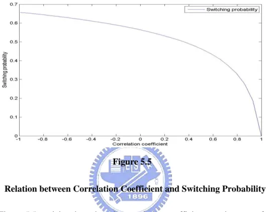
Figure 5.5

Relation between Correlation Coefficient and Switching Probability

Figure 5.5 explains that when the correlation coefficient, , increases from -1 to 1, the switching probability decreases. We know that the brand holder exercises the

switch option depend on the net profit difference of two agents. When the correlation

coefficient increases, the net profit difference decreases. With the same total

switching costs, the brand holder may not be willing to switch the exclusive right

because of decreasing the net profit difference. Finally, there is a negative relation

2. The influence of the commission rate on the probability of switching the exclusive

right in time T is demonstrated in Figure 5.6

Figure 5.6

Relation between Commission Rate and Switching Probability

Figure 5.6 explains when the commission rate, q, increases from 0 to 0.8, the

probability of switching the exclusive right in time T decreases. The brand holder

obtains the cash flow from active agent‟s net profit. Due to the increasing commission

rate, the cash flow and the net profit difference decrease. The brand holder may not be

willing to switch the exclusive right under lower net profit difference. Finally, there is

3. The influence of the Total switching costs on the probability of switching the

exclusive right in time T is demonstrated in Figure 5.7

Figure 5.7

Relation between Total Switching Costs and Switching Probability

Figure 5.7 explains when the total switching costs, K, increase from 0 to 4, the

probability of switching the exclusive right in time T decreases. The total switching

costs are obstacles to entrance. When the obstacles to entrance increase, the brand

holder may not be willing to switch the exclusive agent and the switching probability

decreases. Finally, there is a negative relation between the total switching costs and

4. The influence of the delay cost for idle agent on the probability of switching the

exclusive right in time T is demonstrated in Figure 5.8

Figure 5.8

Relation between Idle Agent’s Delay Cost and Switching Probability Figure 5.8 explains when the idle agent‟s delay cost, _i, increases from 0.01 to 0.08, the probability of switching the exclusive right in time T decreases. The idle

agent‟s delay cost increases, and the idle agent‟s net growth rate decreases. The

probability of switching the exclusive right decreases because the agent with higher

growth rate is easier to be the optimal exclusive agent. Finally, we obtain the negative

5. The influence of the idle agent‟s volatility on the probability of switching the

exclusive right in time T is demonstrated in Figure 5.9

Figure 5.9

Relation between Idle Agent’s Volatility and Switching Probability

Figure 5.9 explains when the idle agent‟s volatility, _i, increases from 0.1 to 0.5, the probability of switching the exclusive right in time T decreases. Because the

volatility means the risk, the brand holder may not switch the exclusive right to the

agent with high volatility. Therefore, when idle agent‟s volatility increases, switching

probability decreases. Finally, we obtain the negative relation between the idle agent‟s

6. The influence of the idle agent‟s growth rate of net profit on the probability of

switching the exclusive right in time T is demonstrated in Figure 5.10

Figure 5.10

Relation between Idle Agent’s Growth Rate and Switching Probability Figure 5.10 explains when the idle agent‟s growth rate, U , increases from 0.03 _i to 0.15, the probability of switching the exclusive right in time T increases. The brand

holder expects that the agent with high growth rate is easier to be the optimal

exclusive agent. Therefore, when the idle agent‟s growth rate increases, the switching

probability increases. Finally, we obtain the positive relation between the idle agent‟s

7. The influence of the active agent‟s delay cost on the probability of switching the

exclusive right in time T is demonstrated in Figure 5.11

Figure 5.11

Relation between Active Agent’s Delay Cost and Switching Probability Figure 5.11 explains when the active agent‟s delay cost, _j, increases from 0.01 to 0.08, the probability of switching the exclusive right in time T increases. The

active agent‟s delay cost increases, and the active agent‟s net growth rate decreases. The brand holder expects that the agent with high growth rate is easier to be the

optimal exclusive agent. The switching probability increases because the active

agent‟s growth rate decreases. Finally, we acquire the positive relation between the active agent‟s delay cost and the switching probability.

8. The influence of the active agent‟s volatility on the probability of switching the

exclusive right in time T is demonstrated in Figure 5.12

Figure 5.12

Relation between Active Agent’s Volatility and Switching Probability Figure 5.12 explains when the active agent‟s volatility, _j, increases from 0.1 to 0.5, the probability of switching the exclusive right in time T increases. Because

the volatility means the risk for the brand holder, he may not switch the exclusive

right to the agent with high volatility. Therefore, when active agent‟s volatility

increases, switching probability increases. Finally, we obtain the positive relation

9. The influence of the active agent‟s growth rate of net profit on the probability of

switching the exclusive right in time T is demonstrated in Figure 5.13

Figure 5.13

Relation between Active Agent’s Growth Rate and Switching Probability Figure 5.13 explains when the active agent‟s growth rate, U , increases from _j 0.03 to 0.15, the probability of switching the exclusive right in time T decreases. The

brand holder expects that the agent with high growth rate is easier to be the optimal

exclusive agent. Therefore, when the active agent‟s growth rate increases, the

switching probability is decreased. Finally, we acquire the negative relation between

the active agent‟s growth rate and the probability of switching.

We acquire all of the relations between each parameter and switching

probability. Table 5.3 shows that how each parameter influences on switching

Table 5.3

Relations between Parameters and Switching Probability

Environmental parameters  K

q

Switching probability

(-)

(-)

(-)

Parameters of idle agent



_i _i u_i

Switching probability

(-)

(-)

(+)

Parameters of active agent



_j



_j

u

_j

Switching probability

(+)

(+)

(-)

To summarize, we can distinguish the results into five factors, which are the net profit

difference, the total switching costs, the cash flow for the brand holder, risk of each

agent and the growth rate of each agent. Switching probability increases when the net

profit difference, the total switching costs and the cash flow for the brand holder

decrease. The brand holder expects that the agent with high growth rate and low

volatility is easier to be the optimal exclusive agent. In addition, we can find that

6. Conclusion and Suggestion

When two agents are competing for the exclusive right, they can earn the different and

uncertain net profits in future. Therefore, claim timing is an important strategy

decision variable for each agent, and it can be optimized with conjecturing the rival‟s

responses. The idle agent has an option to claim the market by sinking the total

switching costs. This paper solves a stochastic real options game in a duopoly agent

market. In order to reduce one dimension, we assume that the optimal strategy

problem is natural homogeneity. In our model, there are some restrictions. First of all,

only one agent can be active in the market. Secondly, we only consider that there are

only two agents competing for the market. Finally, the optimal strategy decisions of

two agents can be converted into optimal switching decisions of the brand holder.

Under these conditions, we can obtain the solutions by using the real options game

method. Using the results, we expect that the agent with high growth rate and low

volatility is a better choice for the brand holder.

This paper analyzes the optimal switching decision under the varied condition

and introduces commission rate in the market. The commission rate does not affect

the results of original model. The results demonstrate how the factors affect hysteresis

and switching probability. The hysteresis increases when the total switching costs, the

decreases. Under the conditions of high commission rate, high correlation coefficient

and high total switching costs, switching is less likely to appear. However, I find out if

the hysteresis increases, it does not mean that the switching probability is less likely

to appear. Switching probability changes depend on each agent‟s parameters and

industry factors.

There are three recommendations for the future research. Firstly, this study

focuses on a duopoly agent market. In real world, there are many agents in an agent

market. We should extend the model to a multiple agents market in future research.

Secondly, in our model, monopolist exists by the exclusive contract. If applying the

model in the other competing market, the patent can also be considered in order to

represent the technical monopolist in the market. Finally, we can apply the model to

the supply chain analysis. For example, Taiwan Semiconductor Manufacturing

Company (TSMC) selects the Original Equipment Manufactures (OEMs) and the

process is one item of the supply chain. Therefore, our model applying to the selection

References

Baldursson, F. M. (1998), “Irreversible Investment under Uncertainty in Oligopoly.”

Journal of Economic Dynamics and Control 22(4), 627-644.

Dixit, A. K. (1989). “Entry and Exit Decisions under Uncertainty.” Journal of

Business, 58(2), 135-157.

Dixit, A. K. and R. S., Pindyck (1994). Investment under Uncertainty, New Jersey:

Princeton University Press.

Grenadier, S. R. (1996). “The Strategic Exercise of Options: Development Cascades

and Overbuilding in Real Estate Markets.‟‟ Journal of Finance 51 (5),

1653-1679.

Harrison, M. J. (1985). Brownian Motion and Stochastic Flow Systems. New York:

John Wiley and Sons.

Hayes, R. H. and W. J., Abernaty (1980), “Managing our Way to Economic Decline.‟‟

Harvard Business Review, July-August, 67-77.

Hayes, R. H. and D. A., Garvin (1982), “Managing as if Tomorrow Mattered.‟‟

Harvard Business Review, May-June, 71-79.

Kensinger, J. (1987). “Adding the Value of Active Management into the Capital

Kulatilaka, N., and L., Trigeorgis. (1994). “The General Flexibility to Switch: Real

Options Revisited.‟‟ International Journal of Finance (6), 78-98.

Lambrecht. B. M. and W. R., Perraudin., (2003). “Real Options and Preemption under

Incomplete Information.‟‟ Journal of Economic Dynamics and Control 27 (4),

619-643.

Margrabe, W. 1978. “The Value of an Option to Exchange One Asset for Another.‟‟

Journal of Financial Economics (18), 7-27.

McDonald, R. L. and D. R., Siegel (1986), “The Value of Waiting to Invest.‟‟

Quarterly Journal of Economics 101 (4), 707–727.

Myers, S. (1987). “Finance Theory and Finance Strategy.‟‟ Midland Corporate

Finance Journal 5, 6 –13.

Shackleton, M. B., A. E., Tsekrekos and R., Wojakowski (2004). “Strategic Entry and

Market Leadership in a Two-player Real Options Game.” Journal of Banking &

Finance 28, 179-201.

Shreve S. (2004). Stochastic Calculus for Finance II: Continuous-Time Model. New

York: Springer.

Slade, M. (1994). “What does an oligopoly maximize?” Journal of industrial

Smets F. (1991). “Exporting versus FDI: The Effect of Uncertainty Irreversibilities

and Strategic Interactions.‟‟ Working Paper, Yale University.

Smit, H. T. J., and L., Trigeorgis (2004). Strategic Investment: Real Options and