THE WINNERLESS COMPETITION PRINCIPLE
SZE-BI HSU AND LIH-ING W. ROEGER
Abstract. We consider a chemostat model of n species of microorganisms competing for k essential, growth-limiting nutrients. Sufficient conditions for the model to possess stable heteroclinic cycles in the limit sets in this model are given. We construct stable heteroclinic cycles that connect the equilibria in the following manner: E1→ E2→ E3→ · · · → En→ E1in which Ei’s are
the one-species equilibria. Therefore the competition among the n species for
k resources is a winnerless competition. Our results show that three essential
nutrients may support any finite number of species and competitive exclusion principle does not hold in the model.
1. Introduction
The chemostat model is a basic model in ecology that describes when two or more populations compete for the same resources, such as a common food supply or a growth-limiting nutrient. It can represent the competition in a simple lake, or as a model of wastewater treatment process [17]. The general chemostat model for
n species competing for k growth-limiting nutrients is as the following [9, 10, 11]:
(1) N0 i(t) = Ni(t)(µi(R1, R2, . . . , Rk) − D), R0 j(t) = D(R0j− Rj(t)) − n X i=1 cjiµi(R1, R2, . . . , Rk)Ni, Ni(0) > 0, Rj(0) ≥ 0, i = 1, 2, . . . , n, j = 1, 2, . . . , k.
Ni(t) denotes the density of species i at time t, and Rj(t) denotes the concentration
of nutrient j at time t; µi(R1, . . . , Rk) is the specific growth rate of species i as a
function of the nutrients Ri’s; D is the flow rate of the chemostat; R0j is the supply
concentration of nutrient j; and cji is the content of nutrient j in species i. The
individual death rates of populations are assumed to be insignificant compared to the flow rate D, i.e., the maximal growth rate of each species, ri, exceeds the
washout rate D since otherwise it cannot survive. According to Liebig’s ”Law of the minimum”, the specific growth rate of species i is determined by the nutrient that is the most limiting, that is
(2) µi(R1, R2, . . . , Rk) = min(f1i(R1), f2i(R2), . . . , fki(Rk)),
Date: July 26, 2007.
2000 Mathematics Subject Classification. 92A15;34C15;34C35.
Key words and phrases. chemostat; resource competition; competitive exclusion; heteroclinic
cycle; competitive system; periodic orbit; winnerless competition.
L.-I. W. Roeger would like to express her gratitude to the people at the National Center for Theoretical Sciences for their hospitality while she visited Taiwan in summers of 2005, 2006, and 2007.
where fji(Rj) is the growth rate of the species i when nutrient Rj is limiting. The
function fji: R+→ R+is assumed to be continuously differentiable and satisfies: fji(0) = 0 and fji0(R) > 0 for R > 0.
For example, we may choose (3) fji(Rj) = riRj
Kji+ Rj, i = 1, 2, . . . , n, j = 1, 2, . . . , k,
which is called the Monod or Michaelis-Menten kinetics for resource up-take. For each species i and each resource j, there is a break-even concentration λji
defined as
fji(λji) = D.
The break-even concentration λjiis the subsistence concentration of each resource
when species i is growth-limited by resource j alone. By the definition of function
fji, we then have fji(x) < D if x < λji; and fji(x) > D if x > λji. In the numerical
example we show later, we assume Monod or Michaelis-Menten kinetics for resource up-take. Then the break-even concentration of species i on resource Rj is
λji= fji−1(D) =
DKji
ri− D.
For model (1), if we form the linear combinations of the variables, we obtain the following equation d dt µ Rj(t) + n X i=1 cjiNi(t) ¶ = D µ R0j− Rj(t) − n X i=1 cjiNi(t) ¶ .
Solving this leads to
Rj(t) + n
X
i=1
cjiNi(t) = R0j+ O(exp(−Dt)).
Therefore, the polygonal set
{(R1, . . . , Rk, N1, . . . , Nn) ∈ Rk+n+ : Rj+ n
X
i=1
cjiNi= R0j, j = 1, . . . , k}
is an invariant and global attracting set for (1). The restriction of (1) to the polygonal set is given by
(4) Ni0(t) = Ni(t) [µi(N1, N2, . . . , Nn) − D] , where µi(N1, N2, . . . , Nn) = µi µ R01− n X j=1 c1jNj(t), R20− n X j=1 c2jNj(t), . . . , R0k− n X j=1 ckjNj(t) ¶ on the set Γ = {(N1, N2, . . . , Nn) ∈ Rn+: n X i=1 cjiNi≤ R0j, j = 1, . . . , k}.
The resources may be easily recovered from the equations
Rj(t) = R0j− n
X
i=1
Huisman and Weissing [9, 10, 11] had used the consumer-resource model (1) to explain biodiversity. They showed by numerical simulations that three or more resources can generate sustained oscillations or even chaotic dynamics of species abundances. For three resources, there are periodic oscillations and the results are verified by Li [12]. When there are five species, chaotic dynamics may occur. Moreover, they showed that three resources can support nine species and five re-sources can support twelve species. Competitive exclusion principle states that at most k species coexist in the competition for k resources. Based on the observation by Huisman and Weissing, the competitive exclusion principle no longer holds for three or more resources in the consumer-resource model (1).
In this manuscript, we find the conditions for the existence of stable heteroclinic cycles of model (1) and use this to extend Huisman and Weissing’s results so that three resources can support any finite species in the way that all species coexist in the form of stable heteroclinic cycle. A heteroclinic contour consists of finitely many saddle equilibria and finitely many heteroclinic orbits connecting these equilibria. The significance of stable heteroclinic cycle is two-fold. First, it is a potential limit set for the dynamics of the system. Second, it is possible to envision the bifurcation of a very long-period periodic orbit from such a cycle [13].
Before we go into details, we introduce the theorem we will apply. The following theorem states the conditions of existence and stability of heteroclinic contours for the canonical Lotka-Volterra model
(5) ˙ai= ai 1 − ai+ N X j6=i ρijaj , i = 1, 2, . . . , n.
This theorem will be generalized to model (1). For the Lotka-Volterra model (5), let’s denote by Ai the equilibrium with only species i exists, i.e. Ai =
(0, 0, . . . , 0, 1, 0, . . . , 0). Assume that there is a heteroclinic orbit Γi connecting
the points Ai and Ai+1, i = 1, 2, . . . , n and An+1= A1. The following result tells
us that the contour or the heteroclinic cycle Γ = ∪n
i=1Γi∪ Ai can be an attractor.
THEOREM 1. [2, Afraimovich et al.] For the Lotka-Volterra competition system
(5), assume that for i = 1, 2, . . . , n,
(6)
ρki> 1, for k 6= i + 1, and ρi+1,i< 1,
ρi,i+1< 2,
ρk,i+1< ρi,i+1, for k 6= i, i + 2,
ν = n Y i=1 µ −1 − ρi,i+1 1 − ρi+1,i ¶ > 1.
(here i + 1 = 1 if i = n). Then there is a neighborhood U of the contour Γ such that for any initial condition a0 = (a0
1, a02, . . . , a0n) in U with a0i > 0, one has
dist(a(t), Γ) → 0 as t → ∞ where a(t) is the orbit going through a0.
The assumptions in Theorem 1 utilized eigenvalues of the Jacobian matrices at
Ai for i = 1, 2 . . . , n. The results can also be applied to the resource-consumer
system (1) and its limiting equations (4). For system (1), consider the limiting equations (4). Denote by Ei the equilibrium with only species i exists, i.e.
Ei= (0, 0, . . . , 0, Ni∗, 0, . . . , 0). Then the eigenvalues of the Jacobian matrix evalu-ated at Eiare (7) σij = ( µj(Ei) − D, for j 6= i, N∗ i ∂µ∂Ni(Eii), for j = i.
Note that σii is always less than zero. Assume that there is a heteroclinic orbit
Γi connecting the points Ei and Ei+1, i = 1, 2, . . . , n and En+1 = E1. Following
Theorem 1, the following result tells us that the contour Γ = ∪n
i=1Γi∪ Ei can be
an attractor for the consumer-resource model (1).
Corollary 1. For the resource-consumer competition system (1), assume that for
i = 1, 2, . . . , n
σik< 0, for k 6= i + 1, and σi,i+1> 0,
(8a)
σi+1,k< σi+1,i, for k 6= i, i + 2,
(8b) ν = n Y i=1 µ −σi+1,i σi,i+1 ¶ > 1. (8c)
(here i + 1 = 1 if i = n). Then there is a neighborhood U of the contour Γ such that for any initial condition a0= (a0
1, a02, . . . , a0n) in U with a0i > 0, one has
dist(a(t), Γ) → 0 as t → ∞ where a(t) is the orbit going through a0.
We will apply Corollary 1 to construct more concrete heteroclinic cycles for the resource-consumer chemostat model (1). This manuscript is organized as follows. In Section 2, the three resources three-species case is reviewed and studied. We show in details how we construct a heteroclinic cycle by embedding the break-even concentrations into the system. In Section 3, We show that the heteroclinic cycle for two-resource n-species case cannot exist. Three resources and more and n species case is presented in Section 4. In Section 5, discussion and possible further work are presented.
2. Three Resources and Three Species
For the consumer-resource model (1), when there are three resources and three species, n = k = 3, Li [12] had done an extended study on the special case when the break-even concentrations of the three species N1, N2, and N3 related to the
three resources S, R, and Q satisfy the following condition:
(9)
λS3< λS2< λS1< S0,
λR1< λR3< λR2< R0,
λQ2 < λQ1 < λQ3< Q0,
where N1 is limited by Q, N2 is limited by S, and N3 is limited by R. The
hy-pothesis (9) also tell us that among all three species N3is the strongest competitor
for resource S and is the weakest competitor for resource Q; N2 is the strongest
competitor for resource Q and the weakest competitor for resource R; and N1 is
the strongest competitor for resource R and the weakest competitor for resource S. Hence, the competition for resources is in a cyclic fashion.
Let the saddle value ν be defined as
(10) ν = −σ13σ21σ32
Li [12] had proved the following results.
THEOREM 2. ([12]) Consider the consumer-resource model (1) when n = k = 3
and its three resources S, R, and Q. If the break-even concentrations satisfy (9) and the saddle value ν < 1, then the heteroclinic cycle E1(Q) → E2(S) → E3(R) → E1 is unstable and there exists a (stable) periodic solution.
The notation E1(Q) → E2(S) → E3(R) → E1will be used throughout the whole
manuscript. It expresses that the heteroclinic cycle is in the order of E1→ E2→ E3→ E1. By adding the resources in the notation, e.g., E1(Q), E2(S), and E3(R),
we simply add extra information for this cycle that N1 is limited by resource Q
near the equilibrium E1, N2 is limited by resource S near the equilibrium E2, and N3 is limited by resource R near the equilibrium E3.
By Corollary 1, we obtain stable condition for the heteroclinic cycle. The results follow.
Corollary 2. Consider the consumer-resource model (1) when n = k = 3 and its
three resources S, R, and Q. If the break-even concentrations satisfy (9) and the saddle value ν > 1, and furthermore, if
(11) σik< 0, for k 6= i + 1, and σi,i+1> 0,
σi+1,k< σi+1,i, for k 6= i, i + 2,
(here i + 1 = 1 if i = 3) then the heteroclinic cycle E1(Q) → E2(S) → E3(R) → E1 is (locally) stable.
There are other ways to produce heteroclinic cycles or periodic solutions. For example, if the break-even concentrations satisfy the following conditions:
(12)
λS1< λS2< λS3,
λR1< λR3< λR2,
λQ2< λQ3 < λQ1,
then we maybe able to find the following heteroclinic cycle
E1(Q) → E2(R) → E3(R) → E1
and a periodic solution depending on the saddle value ν. In addition, we found that if the break-even concentrations for resource S stay fixed in the order λS1< λS2<
λS3, then there are possibly 36 ways to have heteroclinic cycle in the following order
E1→ E2→ E3→ E1.
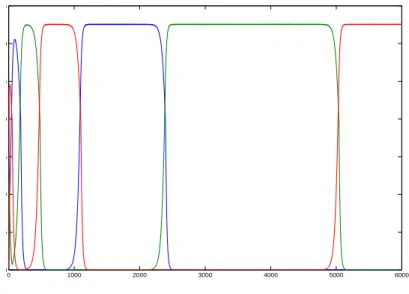
Figure 1 shows an example of a heteroclinic cycle among three species. 3. Three Resources and Four Species
When there are three resources and four species, k = 3 and n = 4, it is possible to have this heteroclinic cycle E1 → E2 → E3 → E4 → E1. There are many
different ways depending on the limiting resources on each species. We may embed the break-even concentrations of the fourth species into the known order (9). By doing this, we are able to find at least 14 cases in which the stable heteroclinic loop E1 → E2 → E3 → E4 → E1 exists. In the following theorem we give one
example that the embedding method will work when the order of the break-even concentrations for the first three species follow the one in the previous section, (9); and the break-even concentrations for species four, λS4, λR4, and λQ4, are
0 1000 2000 3000 4000 5000 6000 0 5 10 15 20 25 30 35
Figure 1. A heteroclinic cycle among three species.
embedded into the the previous order. The resulting stable heteroclinic cycle is stated in the following theorem.
THEOREM 3. For the case of three resources S, R, and Q and four species, if
the break-even concentrations of the four species on the three resources satisfy the following:
(13)
λS3< λS2< λS4 < λS1,
λR4 < λR1< λR3< λR2,
λQ2 < λQ1< λQ4 < λQ3.
Then the assumption (8a) in Corollary can be satisfied. Furthermore, if the eigen-values defined as in (7) satisfy (8b) and (8c), i.e.,
σ13< σ14, σ24< σ21, σ31< σ32, and σ42< σ43 and
ν = σ21σ32σ43σ14 σ12σ23σ34σ41 > 1.
then we have a stable heteroclinic loop in the following order E1(Q) → E2(S) → E3(R) → E4(Q) → E1.
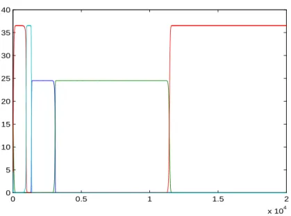
Figure 2 shows an example of a heteroclinic cycle among four species.
Proof. We will apply Corollary 1 in our proof. We show that if assumption (13) is
satisfied, then all conditions in Corollary 1, (8a), (8b), and (8c) are also satisfied so that a stable heteroclinic orbit E1→ E2→ E3→ E4→ E1exists.
Each of the single-species equilibria E1 = (N1∗, 0, 0, 0), E2= (0, N2∗, 0, 0), E3=
(0, 0, N∗
3, 0), and E4= (0, 0, 0, N4∗) must have only one-dimensional unstable
0 0.5 1 1.5 2 x 10⁴ 0 5 10 15 20 25 30 35 40
Figure 2. A heteroclinic cycle among four species.
evaluated at E1, E2, E3, or E4. The eigenvalues σij of each equilibrium are defined
as in (7). They must satisfy σ12 > 0, σ23 > 0, σ34> 0, and σ41 > 0, and σij < 0
for ij 6= 12, 23, 34, and 41.
If E1 = (N1∗, 0, 0, 0) is a steady state at which N1 is limited by Q, then the Q
value at E1 is (14) Q∗ 1= λQ1. Then N∗ 1 can be found to be N∗ 1 = (Q0− λQ1)/cQ1
and the other two corresponding nutrient values are
S1∗= S0− cS1N1∗ and R∗1= R0− cR1N1∗.
In order for E1to be a steady state, i.e., µ1(S1∗, R∗1, Q∗1) − D = 0, we need to have
(15) S∗1 > λS1 and R∗1> λR1.
The Jacobian matrix of (1) when k = 3 and n = 4 at E1 is given by
J(E1) = −N∗ 1fQ10 cQ1 −N1∗fQ10 cQ2 −N1∗fQ10 cQ3 −N1∗fQ10 cQ4 0 σ12 0 0 0 0 σ13 0 0 0 0 σ14 , where f0 Q1= fQ10 (Q∗1) and σ1j= µj(S1∗, R∗1, Q∗1) − D = min(fSj(S1∗), fRj(R∗1), fQj(Q∗1)) − D, j = 2, 3, 4.
We would like to have σ12> 0, σ13< 0, and σ14< 0. In order for σ12> 0, we need
to have
(16) S∗
for σ13< 0, we need to have
(17) S∗
1 < λS3, R∗1< λR3, or Q∗1< λQ3;
and for σ14< 0, we need to have
(18) S∗1 < λS4, R1∗< λR4, or Q∗1< λQ4.
Neither conditions (14)–(18) contradict the assumption (13). We may also con-clude from (14)–(18) that
S∗ 1 > λS1 and R1∗> λR2. That is (19) S 0− λ S1 Q0− λ Q1 > cS1 cQ1 and R0− λ R2 Q0− λ Q1 > cR1 cQ1.
We also obtain that
σ13= fQ3(Q∗1) − D and σ14= fQ4(Q∗1) − D.
If E2= (0, N2∗, 0, 0) is a steady state at which N2is limited by S, then S value
at E2 is (20) S∗ 2 = λS2. Then N∗ 2 can be found to be N2∗= (S0− λS2)/cS2
and the other two corresponding nutrient values are
R∗
2= R0− cR2N2∗and Q∗2= Q0− cQ2N2∗.
In order for E2to be a steady state, i.e., µ2(S2∗, R∗2, Q∗2) − D = 0, we need to have
(21) R∗2> λR2 and Q∗2> λQ2.
The Jacobian matrix of (1) when k = 3 and n = 4 at E2 is given by
J(E2) = σ21 0 0 0 −N∗ 2fS20 cS1 −N2∗fS20 cS2 −N2∗fS20 cS3 −N2∗fS20 cS4 0 0 σ23 0 0 0 0 σ24 , where f0 S2= fS20 (S2∗) and σ2j= µj(S2∗, R∗2, Q∗2) − D = min(fSj(S2∗), fRj(R∗2), fQj(Q∗2)) − D, j = 1, 3, 4.
We would like to have σ21< 0, σ23> 0, and σ24< 0. In order for σ21< 0, we need
to have
(22) S∗
2 < λS1, R∗2< λR1, or Q∗2< λQ1;
for σ23> 0, we need to have
(23) S∗
2 > λS3, R∗2> λR3, and Q∗2> λQ3;
and for σ24< 0, we need to have
(24) S∗
2 < λS4, R∗2< λR4, or Q∗2< λQ4.
Neither conditions (20)–(24) contradict the assumption (13). We may also con-clude from (20)–(24) that
R∗
That is (25) R 0− λ R3 S0− λS2 > cR2 cS2 and Q0− λ Q3 S0− λS2 > cQ2 cS2.
We also obtain that
σ21= fS1(S2∗) − D and σ24= fS4(S2∗) − D.
If E3 = (0, 0, N3∗, 0) is a steady state at which N3 is limited by R, then the R
value at E3 is
(26) R∗3= λR3.
Then N∗
3 can be found to be
N3∗= (R0− λR3)/cR3
and the other two corresponding nutrient values are
S∗
3 = S0− cS3N3∗and Q∗3= Q0− cQ3N3∗.
In order for E3to be a steady state, i.e., µ3(S3∗, R∗3, Q∗3) − D = 0, we need to have
(27) S∗
3 > λS3and Q∗3> λQ3.
The Jacobian matrix of (1) when k = 3 and n = 4 at E3 is given by
J(E3) = σ31 0 0 0 σ32 0 −N∗ 3fR30 cR1 −N3∗fR30 cR2 −N3∗fR30 cR3 −N3∗fR30 cR4 0 0 0 σ34 , where f0 R3= fR30 (R3∗) and σ3j= µj(S3∗, R∗3, Q∗3) − D = min(fSj(S3∗), fRj(R∗3), fQj(Q∗3)) − D, j = 1, 2, 4.
We would like to have σ31< 0, σ32< 0, and σ34> 0. In order for σ31< 0, we need
to have
(28) S∗
3 < λS1, R∗3< λR1, or Q∗3< λQ1;
for σ32< 0, we need to have
(29) S∗
3 < λS2, R∗3< λR2, or Q∗3< λQ2;
and for σ34> 0, we need to have
(30) S∗
3 > λS4, R∗3> λR4, and Q∗3> λQ4.
Neither conditions (26)–(30) contradict the assumption (13). We may also con-clude from (26)–(30) that
λS1> S3∗> λS4 and Q∗3> λQ3. That is (31) S 0− λ S1 R0− λR3 < cS3 cR3 < S0− λ S4 R0− λR3 and Q0− λ Q3 R0− λR3 > cQ3 cR3. We also obtain σ31= fS1(S3∗) − D and σ32= fR2(R∗3) − D.
If E4 = (0, 0, 0, N4∗) is a steady state at which N4 is limited by Q, then the Q value at E4 is (32) Q∗ 4= λQ4. Then N∗ 4 can be found to be N4∗= (Q0− λQ4)/cQ4
and the other two corresponding nutrient values are
S4∗= S0− cS4N4∗ and R∗4= R0− cR4N4∗.
In order for E4to be a steady state, i.e., µ4(S4∗, R∗4, Q∗4) − D = 0, we need to have
(33) S∗
4 > λS4 and R∗4> λR4.
The Jacobian matrix of (1) when k = 3 and n = 4 at E4 is given by
J(E4) = σ41 0 0 0 σ42 0 0 0 σ43 −N∗ 4fQ40 cQ1 −N4∗fQ40 cQ2 −N4∗fQ40 cQ3 −N4∗fQ40 cQ4 , where f0 Q4= fQ40 (Q∗4) and σ4j= µj(S4∗, R∗4, Q∗4) − D = min(fSj(S4∗), fRj(R∗4), fQj(Q∗4)) − D, j = 1, 2, 3.
We would like to have σ41> 0, σ42< 0, and σ43< 0. In order for σ41> 0, we need
to have
(34) S4∗> λS1, R4∗> λR1, and Q∗4> λQ1;
for σ42< 0, we need to have
(35) S∗4 < λS2, R4∗< λR2, or Q∗4< λQ2;
and for σ43< 0, we need to have
(36) S∗4 < λS3, R4∗< λR3, or Q∗4< λQ3.
Neither conditions (32)–(36) contrast to the assumption (13). We may also conclude from (32)–(36) that
S∗ 4 > λS1 and λR2> R∗4> λR1. That is (37) S0− λS1 Q0− λ Q4 > cS4 cQ4 and R0− λR1 Q0− λ Q4 > cR4 cQ4 > R0− λR2 Q0− λ Q4 .
We can also obtain that
σ42= fR2(R∗4) − D and σ43= fQ3(Q∗4) − D.
So far, the four conditions (19), (25), (31), and (37) verify the first assumption (8a) in Corollary 1. With the further assumptions (8b) and (8c), we can then apply
4. Two Resources and n Species
For the consumer-resource model (1), when there are two nutrients and two species in a continuous culture, Hsu et al. [5] had shown that the competition outcomes are similar to the Lotka-Volterra two-species competition models. When there are more than two species, Li and Smith [13] showed that competitive ex-clusion principle holds for the case of 3 species and all of the cases for n > 3 species except for the following case when their break-even concentrations satisfy the following:
(38) λS1< λS2< λS3< · · · < λSn,
λRn< λR,n−1 < · · · < λR2< λR1.
We have additional results for the two-resource n-species case in the following the-orem.
THEOREM 4. Consider the limiting system (4) of the chemostat model with n
species competing for two essential nutrients S and R. Assume that the break-even concentrations satisfy (38). Then there exists no heteroclinic cycle.
Proof. We only need to show that the assumption (8a) in Corollary 1 cannot be
satisfied. The theorem is proved by contradiction.
Suppose there is a heteroclinic cycle connecting all single species equilibria Ei’s.
Without loss of generality we may start the cycle from E1. Let Γij denote the
heteroclinic orbit connecting the two points Ei and Ej. We can summarize the
proof as follows: the heteroclinic orbits Γ12, Γ23, . . . , and Γn−2,n−1 can be found,
but Γn1 does not exist. The cycle is broken between En and E1. Therefore, there
is no heteroclinic cycle.
The proof consists of three parts: (i) if there is a heteroclinic orbit Γk,k+1,
k = 1, 2, . . . , n−1, then species k is limited by resource R, (ii) there is no heteroclinic
orbit Γkm where k + 1 < m ≤ n, and (iii) there is no heteroclinic orbit Γn1.
Claim 1: If there is a heteroclinic orbit Γk,k+1, k = 1, 2, . . . , n − 1, then species
k is limited by the resource R.
If Nk is limited by S, then Sk∗= λS,k and R∗k > λR,k. To guarantee the
hetero-clinic orbit connecting Ekto Ek+1, the k+1st eigenvalue σk,k+1of the Jacobian
ma-trix evaluated at Ek is positive which implies Sk∗> λS,k+1and R∗k > λR,k+1, a
con-tradiction to the assumption (38) that says S∗
k = λSk< λS,k+1. If Nk is R-limited, then S∗ k > λS,k and Rk∗= λR,k. Since λR∗ k < λR,k−1 < λR,k−2< · · · < λR2< λR1, we have σk,k−1< 0, σk,k−2< 0, . . . , σk,2 < 0, and σk,1< 0. S∗
k can be chosen in this way λS,k+1< S∗k < λS,k+2< λS,k+3< · · · < λS,n so that
σk,k+2 < 0, σk,k+3 < 0, . . . , and σk,n < 0. Since Sk∗ > λS,k+1 and R∗k = λR,k >
λR,k+1, we obtain σk,k+1> 0.
Claim 2: There is no heteroclinic orbit connecting Ekto Emwhere k+1 < m ≤ n.
If Nk is S-limited, then Sk∗ = λS,k and Rk∗ > λR,k. σk,m> 0 implies Sk∗> λS,m
and R∗
k > λR,m, a contradiction to (38) which says Sk∗ = λS,k < λS,m. If Nk is
R-limited, then S∗
k > λS,k and Rk∗= λR,k, then σk,k+1< 0 implies Sk∗ < λS,k+1 or
R∗
k < λR,k+1, both are impossible due to (38).
If Nn is R-limited, then R∗n = λR,n and Sn∗ > λS,n. If σn,1 > 0 then Sn∗ > λS,1
and R∗
n> λR,1, a contradiction. If Nnis S-limited, then R∗n> λR,nand Sn∗= λS,n.
If σn,2< 0 then Sn∗< λS,2 or R∗n< λR,2, a contradiction.
So far, the possible heteroclinic orbit is E1(R) → E2(R) → · · · → En−1(R) →
En, but since En→ E1is impossible. We have proved that there is no heteroclinic
loop under the assumption (38). ¤
5. Three or more resources and n species
The following theorem says that three resources can support any finite number of species, which greatly improve the results by Huisman and Weissing [9, 10, 11]. THEOREM 5. Three resources S, R, and Q and n species N1, N2, . . . , Nn.
(39)
λS1< λS2< λS3< · · · < λSn,
λR1< λRn < λR2< λR3< · · · < λR,n−1,
λQ,n−1< λQn< λQ,n−2< · · · < λQ2< λQ1,
Then the assumption (8a) in Corollary 1 can be satisfied. Furthermore, if the eigenvalues defined as in (7) satisfy (8b) and (8c), then we have the following stable heteroclinic loop:
E1(Q) → E2(Q) → · · · → En−2(Q) → En−1(R) → En(S) → E1.
Proof. We only need to verify the following four cases: (i) Ek(Q) → Ek+1, k =
1, . . . , n − 3, (ii) En−2(Q) → En−1, (iii) En−1(R) → En, and (iv) En(S) → E1.
(i) Ek(Q) → Ek+1: Since Nk is limited by Q, we have Q∗k = λQk. Choose Sk∗
and R∗
k such that
λS,k+1< Sk∗< λS,k+2,
λR,k+1< R∗k < λR,k+2.
The Jacobian matrix evaluated at Ek = (0, 0, · · · , Nk∗, 0, · · · , 0) has along the
di-agonal the eigenvalues σkj for j = 1, 2, . . . , n. The eigenvalues are defined as in
(7).
In order to have Ek → Ek+1we need to have σki< 0 for i 6= k+1 and σk,k+1> 0.
For σk,k+1> 0, we need to have
Sk∗> λS,k+1, R∗k > λR,k+1, and Q∗k> λQ,k+1.
This can be done by the way we choose S∗
k, R∗k and Q∗k.
In order to have σki< 0, i 6= k, k + 1, we need
S∗
k < λQi or Rk∗< λRi or Q∗k< λQi.
Since
Q∗
k< λQ,k−1< λQ,k−2< · · · < λQ1,
we have σki< 0 for i = 1, 2, . . . , k − 1. Since
S∗
k < λS,k+2< λS,k+3< · · · < λSn,
we have σki < 0 for i = k + 2, k + 3, . . . , n. Then the eigenvalues of the Jacobian
matrix at Ek satisfy σk,k+1> 0 and σki< 0 for i 6= k + 1.
(ii) En−2(Q) → En−1: Since Nn−2 is limited by Q we have Q∗n−2 = λQ,n−2.
Choose S∗
n−2 and R∗n−2such that
λS,n−1< Sn−2∗ < λSn,
Since S∗
n−2 < λSn we have σn−2,n < 0. Since Q∗n−2 = λQ,n−2 < λQi for i =
1, 2, . . . , n − 3 we have σn−2,i < 0. Then we have σn−1,n−2> 0 and σn−2,i< 0 for
i 6= n − 1, n − 2.
(iii) En−1(R) → En: Nn−1 is limited by R, so R∗n−1 = λR,n−1. Choose S∗n−1
and Q∗
n−1such that
λSn< Sn−1∗ ,
λQn< Q∗n−1< λQ,n−2.
Since Q∗
n−1< λQi for i 6= n − 1, n, we have σn−1,i < 0. Then we have σn−1,n> 0
and σn−1,i< 0 for i 6= n, n − 1.
(iv) En(S) → E1: Nn is limited by S so Sn∗ = λSn. Choose R∗n and Q∗n so that
λRn< Rn∗ < λR2,
λQ1< Q∗n.
Since R∗
n < λR2 < λR3 < · · · < λR,n−1, we have σni < 0 for n 6= 1, n. Then we
have σn1> 0 and σni< 0 for i 6= 1, n. ¤
The previous results can be extended to m + 3 resources and n species.
THEOREM 6. If there are m + 3 resources S, R, Q, P1, . . . , Pm, and n species
N1, N2, . . . , Nn, then under the following conditions
(40)
λS1< λS2< λS3< · · · < λSn,
λR1< λRn< λR2< λR3< · · · < λR,n−1,
λQ,n−1< λQn< λQ,n−2< · · · < λQ2< λQ1,
λPj,1< λPj,2 < λPj,3< · · · < λPj,n, j = 1, 2, . . . , m,
Then the assumption (8a) in Corollary can be satisfied. Furthermore, if the eigen-values defined as in (7) satisfy (8b) and (8c), then we have the following stable heteroclinic loop:
E1(Q) → E2(Q) → · · · → En−2(Q) → En−1(R) → En(S) → E1.
Proof. We only need to verify the following four cases: (i) Ek(Q) → Ek+1, k =
1, . . . , n − 3, (ii) En−2(Q) → En−1, (iii) En−1(R) → En, and (iv) En(S) → E1.
(i) Ek(Q) → Ek+1: Since Nk is limited by Q, we have Q∗k = λQk. Choose Sk∗,
R∗
k, and Pj,k∗ , j = 1, . . . , m such that
λS,k+1< S∗k < λS,k+2,
λR,k+1 < R∗k< λR,k+2,
λPj,k+1< P ∗
j,k< λPj,k+2.
Similar to the arguments before, the eigenvalues of the Jacobian matrix at Ek
satisfy σk,k+1> 0, σki< 0, i 6= k + 1.
(ii) En−2(Q) → En−1: Since Nn−2 is limited by Q we have Q∗n−2 = λQ,n−2.
Choose S∗
n−2, R∗n−2, and Pj,n−2∗ , j = 1, . . . , m such that
λS,n−1< Sn−2∗ < λSn,
λR,n−1< Rn−2∗ ,
λPj,n−1< P ∗
j,n−2< λPj,n.
(iii) En−1(R) → En: Nn−1 is limited by R, so R∗n−1 = λR,n−1. Choose Sn−1∗ ,
R∗
n−1, and Pj,n−1∗ , j = 1, . . . , m such that they satisfy
λSn< Sn−1∗ , λQn< Q∗n−1< λQ,n−2, λPj,n< P ∗ j,n−1. Since Q∗
n−1 < λQi for i 6= n − 1, n, we have σn−1,i < 0. Then we have σn−1,n>
0, σn−1,i< 0, i 6= n, n − 1.
(iv) En(S) → E1: Nn is limited by S, Sn∗ = λSn, and choose Sn∗, R∗n, and Pj,n∗ ,
j = 1, . . . , m satisfying λRn < R∗n< λR2, λQ1 < Q∗n, λPj,1 < P ∗ j,n. Since R∗
n < λR2 < λR3 < · · · < λR,n−1, we have σni < 0 for n 6= 1, n. Then we
have σn1> 0, σni< 0, for i 6= 1, n. ¤
6. Discussion
In this paper we consider the possibility of constructing a stable heteroclinic loop of one-species equlibria for n species competing for k essential resources in a chemostat. The significance of the construction is two- fold. First, it is a potential limit set for the dynamics of the system. Second, it is possible to envision the bifurcation of a very long-period periodic orbit from such a cycle. Thus the existence of the loop may indicate the coexistence state of n species in oscillation form. In [13] Li and Smith conjectured the competitive exclusion principle holds for n species,
n > 2, competing for two essential resources. In Theorem 4 we prove that there
exists no heteroclinic loop for this case. Thus it may give a clue for the future proof of the conjecture. For the case of three essential resources, we construct a stable heteroclinic loop of four species in Theorem 3, thus we extend the result of the paper [12] from three species to four species. Furthermore in Theorem 5 we prove that for three essential resources we are able to construct a stable heteroclinic loop for any finite number of species. Thus our analytic result improves the results of Huisman and Weissing in [9, 10, 11] which are numerical. In fact in Theorem 6, the result can be extended to case of any finite number of species competing for k resources, k > 3.
References
[1] V. S. Afraimovich, S.-B. Hsu, and H.-E. Lin. Chaotic behavior of three competing species of May-Leonard model under small periodic perturbations. International Journal of Bifurcation and Chaos, 11:435–447, 2001.
[2] Valentin S. Afraimovich, M. I. Rabinovich, and P. Varona. Heteroclinic contours in neural ensembles and the winnerless competition principle. International Journal of Bifurcation and Chaos, 14:1195–1208, 2004.
[3] V. S. Afraimovich, V. P. Zhigulin, and M. I. Rabinovich. On the origin of reproducible sequential activity in neural circuits. Chaos, 14:1123–1129, 2004.
[4] S. M. Baer, B. Li, and H. L. Smith. Multiple limit cycles in the standard model of three species competition for three essential resources. J. Math. Biol., 52:745–760, 2006.
[5] S.-B. Hsu, K.-S. Cheng, and S. P. Hubbell. Exploitative competition of microorganisms for two complementary nutrients in continuous cultures. SIAM. J. Appl. Math., 41:422–444, 1981.
[6] S. B. Hsu, S. Hubbell, and P. Waltman. A mathematical theory for single-nutrient competition in continuous cultures of micro-organisms. SIAM. J. Appl. Math., 32:366–383, 1977. [7] J. Hofbauer and K. Sigmund. The Theory of Evolution and Dynamical Systems. Cambridge
University Press, New York, 1988.
[8] S. B. Hsu. Limiting behavior for competing species. SIAM. J. Appl. Math., 34:760–763, 1978. [9] J. Huisman and F. J. Weissing. Biodiversity of plankton by species oscillations and chaos.
Nature, 402:407–410, 1999.
[10] J. Huisman and F. J. Weissing. Biological conditions for oscillations and chaos generated by multispecies competition. Ecology, 82:2682–2695, 2001.
[11] J. Huisman and F. J. Weissing. Fundamental unpredictability in multispecies competition. American naturalist, 157:488–494, 2001.
[12] B. Li. Periodic coexistence in the chemostat with three species competing for three essential resources. Math. Biosci., 174:27–40, 2001.
[13] B. Li and H. L. Smith. How many species can two essential resources support? SIAM. J. Appl. Math., 62:336–366, 2001.
[14] B. Li and H. L. Smith. Periodic coexistence of four species competing for three essential resources. Math. Biosci., 184:115–135, 2003.
[15] G. Laurent, M. Stopfer, R. W. Friedrich, M. I. Rabinovich, A. Volkovskii, and HDI Abarbanel. Odor encoding as an active, dynamical process: Experiments, computation, and theory. ANNUAL REVIEW OF NEUROSCIENCE, 2001, 24:263–297.
[16] M. Rabinovich, A. Volkovskii, P. Lecanda, R. Huerta, HDI Abarbanel, and G. Laurent. Dynamical encoding by networks of competing neuron groups: Winnerless competition . PHYSICAL REVIEW LETTERS, AUG 6, 2001, V8706(N6):8102,U149–U151.
[17] H. L. Smith and P. Waltman. The Theory of the Chemostat, Cambridge Studies in Math. Biol., Cambridge University Press, New York, 1995.
[18] D. Tilman, S. Polasky, and C. Lehman. Diversity, productivity and temporal stability in the economies of humans and nature. J. Environmental Economics and Management, 49:405–426, 2005.
(S.-B. Hsu) Department of Mathematics, National Tsing-Hua University, Hsinchu 300, Taiwan
E-mail address: [email protected]
(L.-I. W. Roeger) Department of Mathematics and Statistics, Box 41042, Texas Tech University, Lubbock, TX 79409, Tel: 806-742-2580, Fax: 806-742-1112