Updating generalized association rules with evolving taxonomies

(1)

Updating Generalized Association Rules with Evolving Taxonomies

Ming-Cheng Tseng1, Wen-Yang Lin2and Rong Jeng3

2

(corresponding author)

1

Institute of Information Engineering, I-Shou University, Kaohsiung 840, Taiwan

2

Department of Computer Science and Information Engineering, National University of Kaohsiung, Kaohsiung 811, Taiwan

E-mail: wylin@nuk.edu.tw

3

Department of Information Management, I-Shou University, Kaohsiung 840, Taiwan

Abstract

Mining generalized association rules among items in the presence of taxonomies has been recognized as an important model for data mining. Earlier work on mining generalized association rules, however, required the taxonomies to be static, ignoring the fact that the taxonomies of items cannot necessarily be kept unchanged. For instance, some items may be reclassified from one hierarchy tree to another for more suitable classification, abandoned from the taxonomies if they will no longer be produced, or added into the taxonomies as new items. Additionally, the analysts might have to dynamically adjust the taxonomies from different viewpoints so as to discover more informative rules. Under these circumstances, effectively updating the discovered generalized association rules is a crucial task. In this paper, we examine this problem and propose two novel algorithms, called Diff_ET and Diff_ET2, to

(2)

Keywords: Data mining, generalized association rules, frequent itemsets, evolving

taxonomies.

1. Introduction

Mining association rules from large databases of business data, such as transaction records, comprises a popular topic within the area of data mining [1][2]. An association rule is an expression of the form X  Y, where X and Y are sets of items. Such a rule reveals that transactions in the database containing items in X tend to also contain items in Y, and the probability, measured as the fraction of transactions that contain X also contain Y, is called the confidence of the rule. The support of the rule is the fraction of the transactions that contain all items in both X and Y. For an association rule to be valid, the rule should satisfy a user-specified minimum support, called ms, and minimum confidence, called mc, respectively. The problem of mining association rules is to discover all association rules that satisfy ms and mc.

In many applications, there are explicit or implicit taxonomies (hierarchies) over the items, so it may be more useful to find associations at different levels of the taxonomies than only at the primitive concept level [13][21]. For example, consider the taxonomies of items in Figure 1.

PDA EPSON EPL MITAC Mio ACER N

Desktop PC PC

IBM TP Systemax V Gateway GE

Figure 1. Example of taxonomies.

It is likely that the association rule,

(3)

does not hold when the minimum support is set to 40%, but the following association rule may be valid,

Desktop PC EPSON EPL.

To the best of our knowledge, all work to date on mining generalized association rules required the taxonomies to be static. However, the taxonomies of items may change as time passes [7], and thus some items will be reclassified from one classification tree to another. For example, IBM TP could be reclassified from PC (Personal Computer) to MC (Mobile Computer) group. Some trees of the taxonomies will be merged together or be split into smaller trees if the items on the trees cannot meet the demands of a new classification. Items will also be abandoned if those items are no longer produced, and new items would be added into the taxonomies. In addition to taxonomies evolution arisen from application background change, the analysts might also like to adjust the taxonomies from different viewpoints to discover more informative rules [11][12]. For example, the analysts would like to add an additional level, say “Product Vendor”, into the taxonomies to discover rules that exploit associations involving such a concept. Under these circumstances, it is important to find a new method to effectively update the discovered generalized association rules.

In this paper, we introduce the problem of updating the discovered generalized association rules under evolving taxonomies. We give a formal problem description and clarify the situations for a taxonomy update in Section 2.

(4)

(2) The process of generating frequent itemsets is very time-consuming.

To be more realistic and cost-effective, it is better to perform the association mining algorithms to generate the initial association rules, and when updates to the taxonomies occur, apply an updating method to re-build the discovered rules. The challenge becomes that of developing an efficient updating algorithm to facilitate the overall mining process. This problem is nontrivial because updates to the taxonomies not only can reshape the concept hierarchy and the form of generalized items, but also may invalidate some of the discovered association rules, thus turning previous weak rules into strong ones, and generating important new rules.

In this paper, we propose two algorithms, called Diff_ET and Diff_ET2 (Differentiating Evolving Taxonomies), for mining the generalized frequent itemsets. These algorithms are capable of effectively reducing the number of candidate sets and database re-scanning, and so they can update the generalized association rules efficiently. A detailed description of the algorithms is given in Section 3.

In Section 4, we evaluate the performance of the proposed algorithms with two leading generalized associations mining algorithms, Cumulate and Stratify [21], using synthetic data. A brief description of previous related work is presented in Section 5. Finally, we summarize our work and propose future investigations in Section 6.

2.

Update of Generalized Association Rules

2.1. Problem description

Let I {i1, i2,…,ip} be a set of items and DB {t1, t2,…,tn} be a set of

transactions, where each transaction tiTID, Ahas a unique identifier TID and a set

of items A (A I). Assume that a set of taxonomy of items, T, is available and is denoted as a set of hierarchies (trees) on IJ, where J {j1, j2,…,jq} represents the

(5)

set of generalized items derived from I. A generalized association rule is an implication of the form A B, where A, B I J, A B , and no item in B is an ancestor of any item in A.

Given a user-specified ms and mc, the problem of mining generalized association rules is to discover all generalized association rules whose support and confidence levels are larger than the specified thresholds. In the literature [13][21], this problem is usually reduced to the problem of finding all frequent itemsets for a given minimum support.

After an initial discovery of all the generalized association rules in DB, let L be the set of all generalized frequent itemsets with respect to ms. As time passes, some update activities may occur to the taxonomies due to various reasons [11][7]. Let

T denote the updated taxonomies. The problem of updating discovered generalized association rules in DB is to find the set of frequent itemsetsLwith respect to the refined taxonomies T .

2.2 Types of taxonomy updates

Intuitionally, the taxonomy evolution and its effect on previously discovered frequent itemsets are more complex than those for data updates because the taxonomy evolution induces item rearrangement in the taxonomies; and once an item, primitive or generalized, is reclassified into another category, all of its ancestor (generalized items) in the old as well as the new taxonomies are affected. In this subsection, we describe different situations for taxonomy evolution, and clarify the essence of frequent itemset updates for each type of taxonomy evolution.

(6)

(1) Item insertion: New items are added to the taxonomies.

(2) Item deletion: Obsolete items are pruned from the taxonomies.

(3) Item renaming: Items are renamed for certain reasons, such as error correction, product promotion, etc.

(4) Item reclassification: Items are reclassified into different categories.

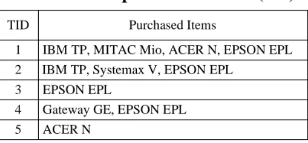
Note that hereafter the term “item”refers to a primitive or a generalized item. In the following, we elaborate each type of evolutions further using the example transactions in Table 1.

Table 1. Example of a database (DB)

1

5 4 3 2

IBM TP, MITAC Mio, ACER N, EPSON EPL TID Purchased Items

ACER N

Gateway GE, EPSON EPL EPSON EPL

IBM TP, Systemax V, EPSON EPL

Type 1: Item insertion. There are different strategies to handle this type of update

operation, depending on whether the inserted item is a primitive or a generalized item.

When the new inserted item is primitive, the support of any itemset consisting of that item is zero, so there is no need to perform association update with respect to the new inserted item until some new transactions consisting of it are added into the source data. On the other hand, if the new item represents a generalization, then only after the new generalization has incurred some item reclassification, will the insertion affect the previously discovered associations.

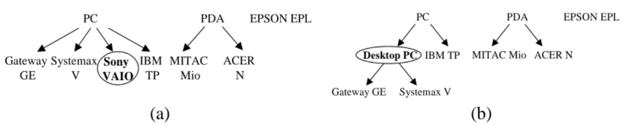
Example 1. Figure 2 shows this type of taxonomy evolution. In Figure 2(a), a new

primitive item “Sony VAIO”is inserted into the generalized item “PC”. Because the new item “Sony VAIO”does not appear in the original transactions, and so is not in the original set of frequent itemsets, we do not have to process it until there is an

(7)

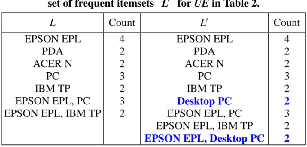
incremental database update. Next, we consider the case of a new generalization insertion. In Figure 2(b), a generalized item “Desktop PC”is inserted as a child of the generalized item “PC”,anditems “Gateway GE”and “Systemax V”arereclassified to the new generalization “Desktop PC”. Since items “Gateway GE”and “Systemax V” already exist in the original database, we must process them to update the generalized frequent itemsets. For illustration, Tables 2(a) and 2(b) show the corresponding extended database before and after the insertion of the generalized item “Desktop PC”, respectively. Let ms 40% 2 transactions). The original set of frequent itemsets L and the new set of frequent itemsets Lare shown in Table 3. Comparing Lwith L, we can observe two new frequent itemsets, {Desktop PC} and {EPSON EPL, Desktop PC}. PC IBM TP Gateway GE Systemax V PDA MITAC Mio ACER N EPSON EPL Sony VAIO

PDA EPSON EPL

MITAC Mio ACER N

Desktop PC PC IBM TP Systemax V Gateway GE (a) (b)

Figure 2. Example of taxonomy evolution caused by item insertion. The inserted new item is: (a) primitive; (b) generalized.

Table 2. Original and updated extended databases derived from Table 1 and Figure 2(b). 1 5 4 3 2

TID Primitive Items Generalized Items Original Extended Database ( ED)

PC, PDA PC

PDA IBM TP, MITAC Mio, ACER N, EPSON EPL IBM TP, Systemax V, EPSON EPL EPSON EPL

Gateway GE, EPSON EPL ACER N PC 1 5 4 3 2

TID Primitive Items Generalized Items Original Extended Database (ED)

PC, PDA PC, Dsektop PC

Gateway GE, EPSON EPL ACER N

PC, Dsektop PC

(8)

Table 3. Original set of frequent itemsets L for ED and the new set of frequent itemsets Lfor UE in Table 2.

L Count L Count EPSON EPL PDA ACER N PC IBM TP EPSON EPL, PC EPSON EPL, IBM TP

4 2 2 3 2 3 2 EPSON EPL PDA ACER N PC IBM TP Desktop PC EPSON EPL, PC EPSON EPL, IBM TP

EPSON EPL, Desktop PC

4 2 2 3 2 2 3 2 2

Type 2: Item deletion. Similar to the insertion case in Figure 2(b), the removal of a

primitive item or generalization would lead to item reclassification, and we shall conduct item support recounting.

Example 2. Figure 3 shows this type of taxonomy evolution, where Figure 3(a) shows

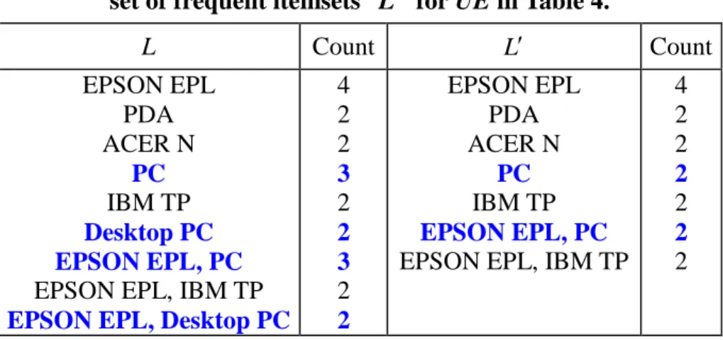
that the primitive item “Gateway GE” is deleted from its top generalized item “Desktop PC”;and Figure 3(b) shows the generalized item “Desktop PC”is deleted from its top generalized item “PC”, and items “Gateway GE”and “Systemax V”are reclassified to “PC”. For illustration, Tables 4(a) and 4(b) show the corresponding extended database before and after the deletion of the primitive item “Gateway GE”, respectively. Let ms40% 2 transactions). From Table 4, the original set of frequent itemsets L and the new set of frequent itemsets Lare shown in Table 5. Comparing

Lwith L, we can observe that two old frequent itemsets, {Desktop PC} and {EPSON EPL, Desktop PC}, become infrequent, and the support counts of {PC} and {EPSON EPL, PC} are changed from 3 to 2. Note that“Gateway GE”is not a candidate since it is not in the new taxonomies. Next, let us consider the deletion of a generalized item from the taxonomies, where Tables 6(a) and 6(b) show the corresponding extended

(9)

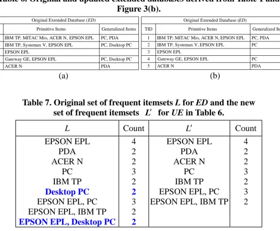
database before and after the deletion of the generalized item “Desktop PC”, respectively. The original set of frequent itemsets L and the new set of frequent itemsets Lare shown in Table 7. Comparing Lwith L, we observe that two old frequent itemsets, {Desktop PC} and {EPSON EPL, Desktop PC}, have been discarded from L.

PDA EPSON EPL

MITAC Mio ACER N Desktop PC PC IBM TP Systemax V Gateway GE PC IBM TP Systemax V Gateway GE Desktop PC PDA MITAC Mio ACER N EPSON EPL (a) (b)

Figure 3. Example of a taxonomy evolution caused by item deletion: (a) primitive; (b) generalized.

Table 4. Original and updated extended databases derived from Table 1 and Figure 3(a). 1 5 4 3 2

Gateway GE, EPSON EPL ACER N PC, Dsektop PC 1 5 4 3 2

PC, PDA PC, Desktop PC

(a) (b)

L Count L Count EPSON EPL PDA ACER N PC IBM TP Desktop PC EPSON EPL, PC

EPSON EPL, IBM TP

4 2 2 3 2 2 3 2 2 EPSON EPL PDA ACER N PC IBM TP EPSON EPL, PC

EPSON EPL, IBM TP 4 2 2 2 2 2 2

(10)

Table 6. Original and updated extended databases derived from Table 1 and Figure 3(b). 1 5 4 3 2

Gateway GE, EPSON EPL ACER N PC, Dsektop PC 1 5 4 3 2

PC, PDA PC

PC

(a) (b)

L Count L Count EPSON EPL PDA ACER N PC IBM TP Desktop PC EPSON EPL, PC EPSON EPL, IBM TP

4 2 2 3 2 2 3 2 2 EPSON EPL PDA ACER N PC IBM TP EPSON EPL, PC EPSON EPL, IBM TP

4 2 2 3 2 3 2

Type 3: Item renaming. Items are renamed for many reasons such as error correction,

product promotion, or other reasons, such as changing a name just for good luck. When items are renamed, we do not have to process the database since the processing codes of the renamed items are the same. Instead, we just replace the discovered frequent itemsets and the association rules with the new names.

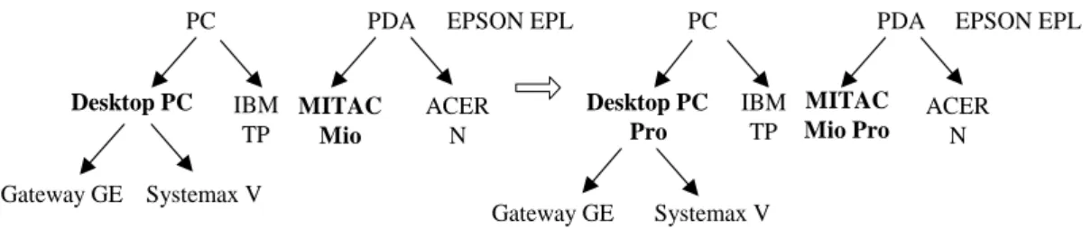
Example 3. Figure 4 shows this type of taxonomy evolution, where the generalized

item “Desktop PC”is renamed to “Desktop PC Pro”, and the primitive item “MITAC Mio”is renamed to “MITAC Mio Pro”.

(11)

PC Desktop PC Pro IBM TP EPSON EPL PDA MITAC Mio Pro ACER N PC Desktop PC IBM TP EPSON EPL PDA MITAC Mio ACER N Gateway GE Systemax V Gateway GE Systemax V

Figure 4. Example of a taxonomy evolution caused by item renaming.

Type 4: Item reclassification. Among all types of taxonomy updates this is the most

profound operation. Once an item, primitive or generalized, is reclassified into another category, all of its ancestor (generalized items) in the old as well as the new taxonomies are affected. That is, the supports of these affected generalized items must be recounted, as do the frequent itemsets containing any one of the affected generalized items.

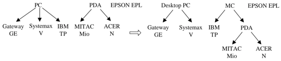
Example 4. In Figure 5, the a reclassified item “IBM TP”willchangethesupport

counts of the generalized items“PC”,“Desktop PC”,and “MC”,andalso affect the support counts ofany itemsetscontaining “PC”,“Desktop PC”,or“MC”.Tables 8(a) and 8(b) show the corresponding extended database before and after the classification of item “IBM TP”. Let ms 40% 2 transactions). The original set of frequent itemsets L and the new set of frequent itemsets Lare shown in Table 9. We observe that there are four new frequent itemsets, {MC}, {Desktop PC}, {EPSON EPL, MC}, and {EPSON EPL, Desktop PC}, added into L, and {PC} and {EPSON EPL, PC} are discarded from L.

(12)

Systemax V PC IBM TP Gateway GE EPSON EPL ACER N PDA MITAC Mio EPSON EPL Desktop PC Systemax V Gateway GE IBM TP ACER N PDA MITAC Mio MC

Figure 5. Example of a taxonomy evolution caused by item reclassification.

Table 8. Original and updated extended databases derived from Table 1 and Figure 5. 1 5 4 3 2

PC, PDA PC

Gateway GE, EPSON EPL ACER N PC 1 5 4 3 2

MC, PDA MC, Dsektop PC

MC, PDA IBM TP, MITAC Mio, ACER N, EPSON EPL

IBM TP, Systemax V, EPSON EPL EPSON EPL

Dsektop PC

(a) (b)

Table 9. Original set of frequent itemsets L for ED and the new set of frequent itemsets Lfor UE in Table 8.

L Count L Count EPSON EPL PDA ACER N PC IBM TP EPSON EPL, PC

EPSON EPL, IBM TP 4 2 2 3 2 3 2 EPSON EPL PDA ACER N MC IBM TP Desktop PC EPSON EPL, MC

EPSON EPL, IBM TP

4 2 2 3 2 2 2 2 2

Note that the basic taxonomy update operations are not commutative; different orders of updates will result in different taxonomy and not all permutations of a given set of updates are feasible. For example, consider the taxonomy in Figure 2. To transfer the taxonomy in (a) into (b), the feasible order is first inserting the new generalization “Desktop PC”and then reclassifying “Gateway GE”and “Systemax V” to “Desktop PC”.

(13)

to the original database; and so according to the above discussions, we only need to consider the taxonomy evolution caused by insertion of generalized items, deletion of items, and reclassification of primitive or generalized items.

3. The Proposed Algorithms

In this section, we look at algorithms for updating discovered frequent itemsets under taxonomy evolution. We first introduce the basic concept, and then describe the details of our two algorithms.

3.1. Algorithm basics

Let ED denote the extended version of DB by adding, in taxonomies T, the ancestors of each primitive item to each transaction, and UE denote another extension of DB by adding generalized items in the updated taxonomies T . A straightforward way to find updated generalized frequent itemsets would be to run any of the current algorithms for finding generalized frequent itemsets, such as Cumulate and Stratify [21], on the updated extended transactions UE. This simple approach, however, ignores the fact that many discovered frequent itemsets are not affected by a taxonomy evolution. Recounting the supports of these unaffected itemsets should be avoided.

Thus, a better approach is to differentiate the unaffected itemsets from the affected ones, and then use them to reduce the work spent on support counting of itemsets. To this end, we must first identify the so called affected primitive items, affected generalizations, and affected transactions, as discussed below. To facilitate

(14)

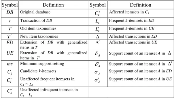
Table 10. Symbol table.

Symbol Definition Symbol Definition

DB Original database  k C Affected itemsets in Ck t Transaction of DB k L Frequent k-itemsets in ED

T Old item taxonomies

k

L Frequent k-itemsets in UE

T  New item taxonomies  Affected transactions in ED

ED Extension of DB with generalized items in T

 Affected transactions in UE

UE Extension of DB with generalized

items in T  A

Support count of an itemset A in 

ms Minimum support setting

A

 Support count of an itemset A in 

k

C Candidate k-itemsets

A

 Support count of an itemset A in ED



k

C Unaffected frequent itemsets in

CkLk

A

 Support count of an itemset A in UE



k

C Unaffected infrequent itemsets in

Ck－Lk

Definition 1. An affected primitive item is a leaf item whose ancestor set changes with

respect to a taxonomy evolution.

Figure 6 shows the procedure for identifying the set of affected primitive items.

1. Let P bethe set of primitive items in TT ; 2. for each item aP do

3. if the ancestors of a in T is different from the ancestors of a in T then

4. Add a to the set of affected primitive items AP; 5. end for

6. return (AP);

Figure 6. Procedure iden_AP(T, T )

Definition 2. A generalized item is called an affected generalization if its descendent

primitive item set changes with respect to a taxonomy evolution.

Figure 7 shows the procedure for identifying the set of affected generalizations.

1. Let G bethe set of generalized items in TT ; 2. for each item aG do

3. if the descendent primitive items of a in T is different from the descendent

(15)

4. Add a to the set of affected items AG; 5. end for

6. return (AG);

Figure 7. Procedure iden_AG(T, T )

For example, consider Figure 5. The generalized items “Desktop PC”, “PC”and “MC”are affected generalizations since their support counts will be changed by the affected primitive item “IBM TP”after the taxonomy evolution. In Figure 2(b), only “Desktop PC”isanewborn affected generalization; “PC”and “PDA”are not affected because the support counts of “PC” come from the three unchanged descendent primitive items“IBM TP”,“Systemax V” and “Gateway GE”,and “PDA”from two unchanged descendentprimitiveitems,“MITAC Mio”and “ACER N”.

Definition 3. For a given itemset A, we say A is an affected itemset if it contains at

least one affected generalization.

Definition 4. A transaction is called an affected transaction if it contains at least one

of the affected primitive items with respect to a taxonomy evolution. Figure 8 shows the procedure for identifying affected transactions.

1. for each transaction tED or t UE do

2. if any item at AP then /* AP: the set of affected primitive items */

3. Mark t as an affected transaction; 4. end for

Figure 8. Procedure iden_AT(ED, UE, AP)

Example 5. Let us consider Figure 5. In Table 8, Transactions 1 and 2 are affected

(16)

Observation 1. The supports of all primitive items in T do not change with respect to

a taxonomy evolution.

Observation 2. The supports of unaffected itemsets do not change with respect to a

taxonomy evolution.

Observation 3. The transactions containing no affected generalization do not affect

the supports of itemsets.

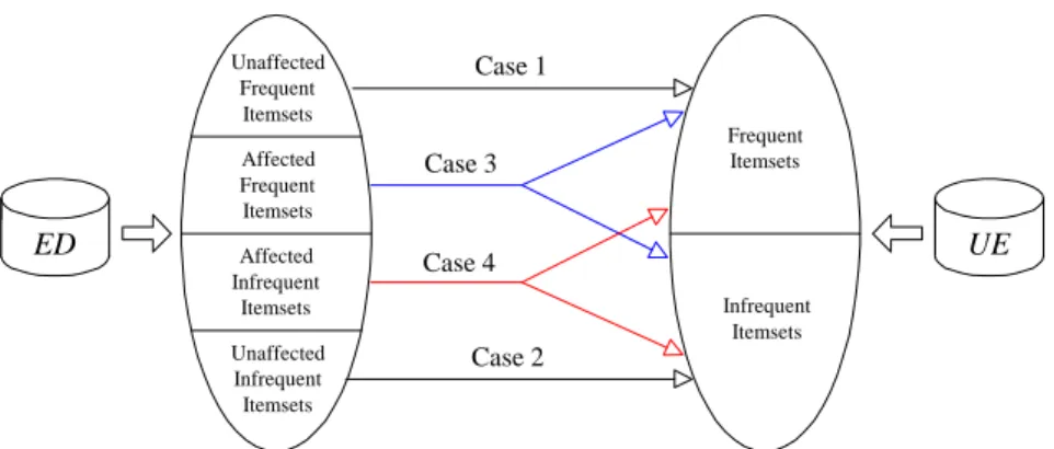
After clarifying the algorithm basics, we will elaborate on how to facilitate the support counting in the mining process. We observe that there are four different cases in dealing with the support counting of an itemset A.

(1) If A is an unaffected itemset and is frequent in ED, then it is also frequent in UE. (2) If A is an unaffected itemset and is infrequent in ED, then it is also infrequent in

UE.

(3) If A is an affected itemset and is frequent in ED, then it may be either frequent or infrequent in UE.

(4) If A is an affected itemset and is infrequent in ED, then it may be either frequent or infrequent in UE.

These four cases are depicted in Figure 9. Note that only Cases 3 and 4 need further database rescanning to determine the support counts of A.

(17)

Case 1 Case 2 Case 4 Case 3 ED _Affected UE Infrequent Itemsets Affected Frequent Itemsets Unaffected Frequent Itemsets Unaffected Infrequent Itemsets Infrequent Itemsets Frequent Itemsets

Figure 9. Four cases arising from the taxonomy evolution.

3.3. Algorithm Diff_ET

Based on the aforementioned concepts with the level-wise approach widely used in most efficient algorithms to generate all frequent k-itemsets, we propose an algorithm called Diff_ET, which processes only the updated extended database UE. The main process of Diff_ET is presented as follows.

First, add generalized items in the new item taxonomy T into the original database DB to form UE and identify affected generalizations for dividing candidate itemsets. Next, let candidate 1-itemsets C be the set of items in the new item1

taxonomies T . That is, all items in T are candidate 1-itemsets. Then load the original frequent 1-itemsets L1and divide C into three subsets:1

 1 C , C , and1  1 C .  1

C consists of unaffected 1-itemsets in L1, and C1 contains affected 1-itemsets, and 

1

C is composed of unaffected 1-itemsets not in L1, where C is for Case 1,1  1

C for

Cases 3 and 4, and C for Case 2. According to Case 2,1  1

C is infrequent; therefore, 

1

C is pruned. Then compute the support counts of each 1-itemset in C₁ over only transactions that contain affected items in UE. After this, we create new frequent

(18)

procedure until no frequent k-itemsetsLkare created.

The Diff_ET algorithm is shown in Figure 10.

Input: (1) DB: the database; (2) the minimum support setting ms; (3) T: the old

item taxonomies; (4) T : the new item taxonomies; (5) L: the set of original frequent itemsets.

Output: L: the set of new frequent itemsets with respect to T . Steps:

1. Add generalized items in T into the original database DB to form UE; 2. AGiden_AG(T, T ); /* Identifing affected items */

3. k 4. repeat

5. if kthen Generate C from₁ T ; 6. elseC_kapriori-gen(L_k_₁);

7. Delete any candidate inC that consists of an item and its ancestor;_k

8. Load original frequent itemsetsL ;_k

9. _Divide

k

C into three subsets: C_k, C_k, and C_k; /* C_k consists of unaffected itemsets inL , and_k C_kcontains affected itemsets, and



k

C contains unaffected itemsets not inLk */

10. _{Count the occurrences of each itemset A in} 

k

C over UE; 11.

k

L{AC_ksupUE(A)ms}Ck;

12. until Lk

13. LUkLk;

Figure 10. Algorithm Diff_ET.

3.3.1. An example for Diff_ET

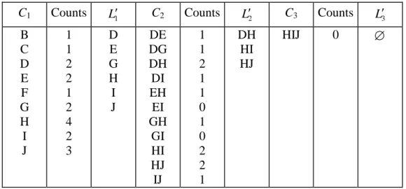
Consider the taxonomies in Figure 11, where item “A”standsfor“PC”,“B”for “Gateway GE”,“C”for“Systemax V”,“D”for“IBM TP”“E”for“PDA”,“F”for “MITAC Mio”,“G”for“ACER N”,“H”for“EPSON EPL”, “I”for“Desktop PC”, “J”for“MC”and“K”for“ASUS P2X”. Let ms25% 2 transactions). Tables 11 and 12 show the summary of candidates, counts and frequent itemsets in ED and UE, respectively.

(19)

consists of unaffected 1-itemsets C₁{D, E, G, H} in L1; the second contains

affected generalized 1-itemsets C₁{I, J},where “I”and “J”are new generalized items; and the third consists of unaffected 1-itemsets C₁{B, C, F} not in L1. Since

all 1-itemsets in C₁ are frequent and do not change their supports in UE, we do not need to process them; we only have to process generalized 1-itemsets {I, J}. According to Case 2, C₁ is infrequent and so is pruned directly. Next, UE is scanned for {I, J}. After comparing the supports of {I} and {J} to ms, the new set of frequent 1-itemsets Lis {D, E, G, H, I, J}.1

Next, we use Lto generate candidate 2-itemsets₁ C , obtaining₂ C₂{DE, DG,

DH, DI, EH, EI, GH, GI, HI, HJ, IJ}. However, only {DI}, {EI}, {GI}, {HI}, {HJ}, and {IJ} undergo support counting, because the others are composed of unaffected items. Note that 2-itemsets {AD, EG} in ED and {DJ, EG, EJ, GJ} in UE are deleted due to the existence of an item-ancestor relationship. After that, the procedure of generating frequent 2-itemsets is the same as that for generatingL₁. The new set of frequent 2-itemsets Lis {DH, HI, HJ}.₂

Finally, we use the same approach to generateL₃, obtaining L₃. The overall

(20)

1 5 4 3 2 D, F, G, H J, E D, C, H J, I TID Primitive Items Generalized Items G B, H H I J, E Updated Extended Database (UE)

1 5 4 3 2 D, F, G, H A, E D, C, H A TID Primitive Items Generalized Items G B, H H A E Original Extended Database (ED)

H C I B J D G E F H C A D B G E F

Figure 11. Example of mining generalized association rules caused by item reclassification.

Table 11. Summary for candidates, counts and frequent itemsets generated from ED.

C1 Counts L1 C2 Counts L2 C3& L3

A B C D E F G H 3 1 1 2 2 1 2 4 A D E G H AE AG AH DE DG DH EH GH 1 1 3 1 1 2 1 1 AH DH 

Table 12. Summary for candidates, counts and frequent itemsets generated from UE.

C1 Counts L₁ C2 Counts L₂ C3 Counts L₃

B C D E F G H I J 1 1 2 2 1 2 4 2 3 D E G H I J DE DG DH DI EH EI GH GI HI HJ IJ 1 1 2 1 1 0 1 0 2 2 1 DH HI HJ HIJ 0 

(21)

B, C, D, E, F, G, H, I, J

D, E, G, H

D, E, G, H, I, J

DE, DG, DH, DI, EH, EI, GH, GI, HI, HJ, IJ DH HIJ DH, HI, HJ I, J 2 C Generate C₂ Affected C₂

DI, EI, GI, HI, HJ, IJ 3 C Generate Scan UE Scan UE 1 C Generate 2 L Generate L₁ Load B, C, F Affected C₁ 3 L  3 C 2 L Generate L₃ DE, DG, EH, GH 2 L in not inL₂ Unaffected 2 C DI EI GI HI HJ IJ 1 0 0 2 2 1 I J 3 2 1 L in 1 L not in Unaffected C₁ L1 1 L

(22)

3.4. Algorithm Diff_ET2

We also propose another algorithm called Diff_ET2, which simultaneously processes both the original extended database ED and the updated extended database

UE. As stated previously, only Cases 3 and 4 need further database rescanning to

determine the support counts of itemset A. For Case 3, we have to rescan the affected transactions in ED and UE, to decide whether A is frequent or not. As for Case 4, the following lemma provides an effective pruning strategy to reduce the number of candidate itemsets and so avoid unnecessarily database rescans.

Lemma 1. If an affected itemset AL (frequent itemsets in ED) and A  , then AA

L(frequent itemsets in UE).

Proof. If A L, then  |ED| ms. Note that |UE| |ED| and |_A | ||. Hence,

A

 + (A A  ) |ED| ms |UE| ms. Thus, A A L. 

Thus in Case 4, we scan the affected transactions, in ED and in UE, respectively, to count the occurrences of A. If the support counts of A in are greater than those in , then we have to scan UE to decide whether A is frequent or not.

Example 6. Consider Figure 13. Let ms60% (3 transactions). Then item “I”is not

frequent in ED. Hence, are not available in L. From_{I} and , we have  _{I} 1,

{I}

0 and _{I} _{I} 1, i.e., _{I} ,_{I} “I” is infrequent in UE according to Lemma 1. Therefore, we do not need to scan the transactions in UEto determine whether item “I”isfrequent or not. This reduces the number of candidates before scanning UE.

(23)

H G E F A D C I K B H G E F A D C I B 1 5 4 3 2 F, H, K E H TID Primitive Items Generalized Items B, C, D, H D, G, H D, F, H A, E A, I Updated Extended Database (UE)

A, E  1 5 4 3 2 F, H, K A, I, E H TID Primitive Items Generalized Items B, C, D, H D, G, H D, F, H A, E A, I Original Extended Database (ED)

A, E 

Figure 13. Example of mining generalized association rules caused by item reclassification.

Based on the aforementioned concept, the main process of Diff_ET2 is presented as follows.

First, add all generalized items in the old and new item taxonomies T and T into the original database DB to form ED and UE, respectively, and identify affected primitive items and affected generalizations. We identify affected primitive items for affected transactions. Next, let the set of candidate 1-itemsets C be the set of items1

in the new item taxonomies T , i.e. all items in T are candidate 1-itemsets. Then load the original frequent 1-itemsets L1 and divide C into the three subsets of1

 1 C , 

1

C , and C ; where₁ C₁ consists of unaffected 1-itemsets in L1, C1 contains

affected 1-itemsets, and C₁ contains unaffected 1-itemsets not in L1. According to

Case 2, C is infrequent, so₁ C₁ is pruned directly. After dividing C , we first1

compute the support counts of each 1-itemset A in C1 over the affected transactions

of  and ; letting the values be  andA , respectively. Then, for eachA

1-itemset A that is in L1and C , i.e., A1   1

C L , calculate the support count1 A

(24)

which are frequent in C . For the next cycle we generate candidates 2-itemsets C₁ 2

from Land repeat the same procedure for generating₁ Luntil no frequent₁ k-itemsetsLkare created.

The Diff_ET2 algorithm is shown in Figure 14.

Input: (1) DB: the database; (2) the minimum support setting ms; (3) T: the old

item taxonomies; (4) T : the new item taxonomies; (5) L: the set of original frequent itemsets.

Output: L: the set of new frequent itemsets with respect to T . Steps:

1. Add generalized items in T into the original database DB to form ED; 2. Add generalized items in T into the original database DB to form UE; 3. APiden_AP(T, T ); /* Identifing affected items */

4. AGiden_AG(T, T ); /* Identifing affected generalizations */ 5. Call iden_AT(ED, UE, AP); /* Identifing affected transactions */ 6. k

7. repeat

8. if kthen Generate C from1 T ;

9. elseC_kapriori-gen(L_k_₁);

10. Delete any candidate inC that consists of an item and its ancestor;_k

11. Load original frequent itemsetsL ;_k

12. _Divide _{C into three subsets:}_k _C_k_, _C_k_{, and} _C_k_; _/* _C_k _{consists of} unaffected itemsets inL , and_k C_kcontains affected itemsets, and



k

C contains unaffected itemsets not inLk */

13. _{Count the occurrences of each itemset A in} 

k

C over ; 14. _{Count the occurrences of each itemset A in} 

k

C over ; 15. _{for each itemset A}_ 

k

C L_k do /* Case 3 */ 16. Calculate _A  _A  _A ;_A

17. for each itemset A L and_k _A  do_A /* Case 4 & Lemma 1 */ 18. Count the occurrences of A over UE -;

19. Add the count into ;A

20. end for

21.

k

L{AC_ksupUE(A)ms}Ck;

22. until Lk

23. LUkLk;

(25)

3.4.1. An example for Diff_ET2

Consider Figure 13 and let ms 60% 3 transactions). The set of frequent itemsets L {A, D, E, H, AE, AH, DH, EH, AEH}. Note that item “K” is not interesting and is deleted from the old taxonomy; therefore, we do not add its ancestors to UE.

The Diff_ET2 algorithm first divides all 1-itemsets in C1into three subsets: one

consists of unaffected 1-itemsets C₁{D, E, H} in L1; the second contains affected

generalized 1-itemsets C₁{A, I},where“A”is frequent in L1, while “I”is not; and

the third consists of unaffected 1-itemsets C₁{B, C, F, G} not in L1. Since

1-itemsets in C1 are frequent and do not change their supports in UE, we do not

need to process them; we only need to process generalized 1-itemsets {A, I}. According to Case 2, C₁ is infrequent and pruned directly. Next, Transaction 1 in

ED and UE is scanned since the transaction is affected by item “L”.We then subtract the support countsofitem “A”inand add their support counts in . For example, we have _{A} _{A}  _{A} _{A} . Because _{I} _{I} 1, i.e.,

{I}

 ,{I} item “I”isinfrequent in UE according to Lemma 1. Therefore, we do not

need to scan the transactions in UEto determine whether item “I”isfrequentor notAftercomparing thesupportsof“A”to ms, the new set of frequent 1-itemsets L₁

is {A, D, E, H}.

Next, we use Lto generate candidate 2-itemsets₁ C , obtaining₂ C₂{AE, AH,

(26)

procedure of generating frequent 2-itemsets is the same as that for generating L1. The

new set of frequent 2-itemsets Lis {AH, DH, EH}. Finally, we use the same2

approach to generate L₃, obtaining L₃.

4. Performance Evaluation

In order to examine the performance of Diff_ET and Diff_ET2, we conducted experiments to compare them with Cumulate and Stratify, using the synthetic dataset generated by the IBM data generator [2], and Microsoft foodmart2000 database (Foodmart for short), a sample supermarket data warehouse provided in MS SQL 2000. The data for Foodmart is drawn from sales_fact_1997, sales_fact_1998 and sales_fact_dec_1998 in foodmart2000. The corresponding item taxonomy consists of three levels: There are 1560 primitive items in the first level (product), 110 generalized items in the second level (product_subcategory), and 47 generalized items in the top level (product_category). The comparisons were evaluated according to certain aspects, including the differences in minimum supports, transaction sizes and evolution degree. Here, the evolution degree is measured by the fraction of generalized items that contain affected generalized items. In the implementation of each algorithm, we also used two different support counting strategies: one with the horizontal counting [1][2][3][18] and the other with the vertical intersection [19][24]. For the horizontal counting, the algorithms are denoted as Cumulate(H), Stratify(H), Diff_ET(H), and Diff_ET2(H). For the vertical intersection counting, they are denoted as Cumulate(V), Stratify(V), Diff_ET(V), and Diff_ET2(V). The parameter settings are shown in Table 13. All experiments were performed on an Intel Pentium-IV 2.80GHz with 2GB RAM, running on Windows 2000. Note that in some figures,

(27)

vertical scales are in logarithmic representation for better resolution.

Table 13. Default parameter settings for synthetic data generation.

Default value Parameter

Synth1 Foodmart |DB| Number of original transactions 177783 62568

|t| Average size of transactions 16 12

N Number of items 231 1717

R Number of groups 30 47

L Number of levels 3 3

F Fanout 5 14

Minimum supports: We first compared the performance of these four algorithms

with varying minimum supports at constant evolution degree 7.9% for Synth1 and 2.5% for Foodmart, and the number of transactions, fanout and groups are set to default values. The experimental results are shown in Figures 15 and 16 for dataset Synth1 and Foodmart, respectively. In Figure 15, at ms 0.5%, Diff_ET(V) performs 101% and 416% faster than Cumulate(V) and Stratify(V), respectively, while Diff_ET(H) performs 257% and 358% faster than Cumulate(H) and Stratify(H), respectively. In Figure 16, at ms 0.075%, Diff_ET(V) and Diff_ET2(V) perform 41% faster than Cumulate(V), and overwhelms Stratify since Stratify took too much time in finding top itemsets, while Diff_ET(H) and Diff_ET2(H) perform 44% and 55% faster than Cumulate(H), respectively. Among our algorithms, Diff_ET(V) and Diff_ET2(V) perform better than Diff_ET(H) and Diff_ET2(H). The performance difference between Diff_ET and Diff_ET2 is not significant.

(28)

1 10 100 1000 10000 0.5 1 1.5 2 2.5 3 3.5 ms % R u n ti m e (s ec .) Cumulate(V) Stratify(V) Diff_ET 2(V) Diff_ET (V) Cumulate(H) Stratify(H) Diff_ET 2(H) Diff_ET (H) log

Figure 15. Performance comparison of Diff_ET, Diff_ET2, Cumulate, and Stratify for different ms over Synth1.

1 10 100 1000 10000 0.05 0.10 0.15 0.20 0.25 0.30 0.35 ms % R u n ti m e (s ec .) Cumulate(V) Stratify(V) Diff_ET 2(V) Diff_ET (V) Cumulate(H) Stratify(H) Diff_ET 2(H) Diff_ET (H) log

Figure 16. Performance comparison of Diff_ET, Diff_ET2, Cumulate, and Stratify for different ms over Foodmart.

Transaction sizes: We then compared the four algorithms under varying transaction

sizes at ms 1.0% with constant affected item percent 7.9% for Synth1 and at ms 0.1% with affected item percent 2.5% for Foodmart. The other parameters are set to default values. Since Stratify exhibits poor performance at ms0.1% for Foodmart as shown in Figure 16, we only compare our algorithms with Cumulate. The results are depicted in Figures 17 and 18 for Synth1 and Foodmart, respectively. It can be seen

(29)

that all algorithms exhibit linear scalability. In Figure 17, the vertical version of our algorithms performs better than the vertical version of Cumulate and Stratify, and Diff_ET2(H) performs better than Stratify(V) under 100,000 transactions. In Figure 18, Diff_ET and Diff_ET2(V) overwhelm Cumulate(V), and Diff_ET(H) and Diff_ET2(H) perform better than Cumulate(H), while Diff_ET2(H) beats Cumulate(V) over 40,000 transactions. 1 10 100 1000 2 4 6 8 10 12 14 16 18 Number of transctions (x 10,000) R u n ti m e (s ec .) Cumulate(V) Stratify(V) Diff_ET 2(V) Diff_ET (V) Cumulate(H) Stratify(H) Diff_ET 2(H) Diff_ET (H) log

Figure 17. Performance comparison of Diff_ET, Diff_ET2, Cumulate, and Stratify different transactions over Synth1.

(30)

60 80 100 120 140 1 2 3 4 5 6 7 Number of transctions (x 10,000) R u n ti m e (s ec .) Cumulate(V) Diff_ET 2(V) Diff_ET (V) Cumulate(H) Diff_ET 2(H) Diff_ET (H)

Figure 18. Performance comparison of Diff_ET, Diff_ET2, Cumulate, and Stratify different transactions over Foodmart.

Evolution degree: Finally, we compared the algorithms under varying degrees of

evolution with ms 1.0% for Synth1 and with ms 0.1% for Foodmart. The other parameters were set to default values. Since Stratify presents poor performance at ms 0.1% for Foodmart, we only compare our algorithms with Cumulate. Intuitively, with more affected primitive items, there should be more affected transactions; with more affected generalizations, there should be more affected itemsets. In the experiments, the affected primitive items and affected generalizations were reclassified randomly with some new groups, and the results are depicted in Figures 19 and 20 for Synth1 and Foodmart, respectively. As the results show, our algorithms are greatly affected by the degree of evolution, whereas Cumulate and Stratify exhibit steady performance. In Figure 19, Diff_ET(V) beats Cumulate under 55% of evolution and Diff_ET2(V) only under 25%, while Diff_ET(H) and Diff_ET2(H) perform almost the same under 3%. In Figure 20, Diff_ET2(V) performs better than Cumulate(V) under 31% of evolution, while Diff_ET2(H) performs better than

(31)

Cumulate(H) under 31% of evolution. In both figures, Diff_ET(V) and Diff_ET2(V) exhibit better performance than Diff_ET(H) and Diff_ET2(H). Note that Diff_ET overwhelms Diff_ET2 most of the time since Diff_ET2 needs to scan ED and UE simultaneously, and the advantage of Lemma 1 for Diff_ET2 disappears when the number of affected transactions increases.

10 100 1000 10000 0 10 20 30 40 50 60 70 80 Evolution % R u n ti m e (s ec .) Cumulate(V) Stratify(V) Diff_ET 2(V) Diff_ET (V) Cumulate(H) Stratify(H) Diff_ET 2(H) Diff_ET (H) log

Figure 19. Performance comparison of Diff_ET, Diff_ET2, Cumulate, and Stratify for different degrees of evolution over Synth1.

40 80 120 160 200 10 15 20 25 30 35 40 45 Evolution % R u n ti m e (s ec .) Cumulate(V) Diff_ET 2(V) Diff_ET (V) Cumulate(H) Diff_ET 2(H) Diff_ET (H)

(32)

5. Related Work

The problem of mining association rules in the presence of taxonomy information was addressed first by Han et al. [13] and Srikant et al. [21], independently. In [21], the problem was referred to mining generalized association rules, aiming to find associations among items at any level of the taxonomies under the minimum support and minimum confidence constraints. In [13], the problem mentioned was somewhat different from that considered in [21] because they generalized the uniform minimum support constraint to a form of assignment according to level, i.e., items at the same level received the same minimum support. The objective was to develop mining associations level-by-level in a fixed hierarchy. That is, only associations among items on the same level were examined progressively from the top level to the bottom.

The problem of updating association rules incrementally was first addressed by Cheung et al. [4]. They developed the essence of updating the discovered association rules when new transaction records are added into the database over time, and they proposed an algorithm called FUP (Fast UPdate). They further examined the maintenance of multi-level association rules [5], extending the model to incorporate the situations of deletion and modification [6]. Their approaches [5][6], however, did not consider the generalized items, and hence could not discover generalized association rules.

Subsequently, a number of techniques have been proposed to improve the efficiency of incremental mining algorithms [14][15][20][22], although all of them were confined to mining associations between primitive items. The problem of maintaining generalized associations incrementally has been recently investigated [23], wherein the model of generalized associations was extended to that with

(33)

non-uniform minimum support.

In summary, all work on mining generalized association rules required the taxonomies to be static and ignored the fact that taxonomies of items may change over time or be adjusted by the analysts [11][7]. This paper is the first, to our knowledge, to propose methods for solving this problem.

6. Discussions and Conclusions

In this paper we have investigated the problem of updating generalized association rules under evolving taxonomies. We presented two algorithms, Diff_ET and Diff_ET2, for updating generalized frequent itemsets. Empirical evaluation showed that both algorithms are effective and have good linear scale-up characteristic. Before we come to an end, we like to point out that our algorithms can be applied to some extensions of the problem concerned in this paper. Firstly, though we have assumed, for simplicity, the item taxonomy is arranged as hierarchy tree, the proposed algorithms indeed can handle the taxonomy organized as directed acyclic graph or lattice. Secondly, the proposed algorithms can be applied to other types of data sources not in transactional format. As founded in [9], the process of discovering knowledge from databases or data warehouses usually involves some preliminary steps including relevant data extraction, cleansing, and transformation to prepare the data workable for applying the appropriate mining algorithms or tools. In this context, our algorithms can be applied to update previously discovered patterns once the relevant data have been prepared in transactional format.

(34)

incorporates incremental database updates and fuzzy taxonomic structure. Another important direction is on embedding the frequent pattern maintenance scheme into a data mining platform. An example is on-line discovery of multi-dimensional association rules from databases or data warehouses [15]. The realization of such systems heavily depends on an auxiliary repository depicting to some extent the statistics of the patterns to be mined. Previous work toward this avenue includes J. Han on utilizing OLAP cube to create an OLAP-like mining environment [10][15], iceberg cube [8], OLAM cube [16], and materialized data mining views [7], etc. Efficiently maintaining this auxiliary repository with respect to data source update and/or taxonomic structure (or more general, schema) evolution then become another important research issues.

Acknowledgement

We would like to acknowledge many constructive comments from the anonymous referees. This work was supported by the National Science Council of ROC under grant NSC 94-2213-E-390-006.

References

[1] R.Agrawal,T.Imielinski,and A.Swami,“Mining association rulesbetween sets ofitemsin largedatabases,”Proc. 1993 ACM-SIGMOD Intl. Conf. Management of Data, 1993, pp. 207-216.

[2] R.Agrawaland R.Srikant,“Fastalgorithmsformining association rules,”Proc. 20th Int. Conf. Very Large Data Bases, 1994, pp. 487-499.

[3] S. Brin, R. Motwani, J.D. Ullman, and S. Tsur, "Dynamic itemset counting and implication rules for market basket Data," SIGMOD Record, Vol. 26, 1997, pp.

(35)

255-264.

[4] D.W. Cheung, J. Han, V.T. Ng, and C.Y. Wong. “Maintenance of discovered association rules in large databases:An incremental update technique,” Proc.

1996 Int. Conf. Data Engineering, 1996, pp.106-114.

[5] D.W. Cheung, V.T. Ng,B.W.Tam,“Maintenanceofdiscovered knowledge:a case in multi-level association rules,” Proc. 1996 Int. Conf. Knowledge

Discovery and Data Mining, 1996, pp. 307-310.

[6] D.W. Cheung, S.D. Lee, and B. Kao, “A general incremental technique for maintaining discovered association rules,”Proc. DASFAA'97, 1997, pp. 185-194.

[7] B. Czejdo, M. Morzy, M. Wojciechowski, and M. Zakrzewicz, “Materialized views in data mining,”Proc. 13th Intl. Workshop on Database and Expert

Systems Applications, 2002, pp. 827-831.

[8] M. Fang, N. Shivakumar, H. Garcia-Molina, R. Motwani, J.D. Ullman, “Computing iceberg queries efficiently,”Proc. 24th Intl. Conf. Very Large Data

Bases, 1998, p.299-310.

[9] U. Fayyad, G. Piatetsky-Shapiro, and P. Smyth,“TheKDD processforextracting usefulknowledgefrom volumesofdata,”Communications of the ACM, Vol. 39,

No. 11, 1996, pp. 27–34.

[10] J. Han, “OLAP mining: An integration of OLAP with data mining,”Proc. IFIP

Conf. Data Semantics, 1997, pp. 1-11.

[11] J. Han, Y. Cai, and N. Cercone, “Knowledge discovery in databases: An attribute-oriented approach,”Proc. 18th Intl. Conf. Very Large Data Bases, 1992, pp. 547-559.

(36)

Discovery in Databases (KDD’94), 1994, pp. 157-168.

[13] J. Han and Y. Fu, “Discovery of multiple-level association rules from large databases,”Proc. 21st Int. Conf. Very Large Data Bases, 1995, pp. 420-431.

[14] T.P. Hong, C.Y. Wang, and Y.H. Tao, “Incremental data mining based on two support thresholds,” Proc. 4th Int. Conf. Knowledge-Based Intelligent Engineering Systems and Allied Technologies, 2000, pp.436-439.

[15] M. Kamber, J. Han, and J. Y. Chiang, “Metarule-guided mining of multidimensional association rules using data cubes,”Proc. 3rd Intl. Conf.

Knowledge Discovery and Data Mining (KDD'97), 1997, pp. 207-210.

[16] W.Y. Lin, J.H. Su, and M.C. Tseng, “OMARS: The framework of an online multi-dimensional association rules mining system,”ICEB 2nd Intl. Conf.

Electronic Business, Taipei, Taiwan, 2002.

[17] K.K. Ng and W. Lam, “Updating of association rules dynamically,”Proc. 1999

Intl. Symp. Database Applications in Non-Traditional Environments, 2000, pp.

84-91.

[18] J.S. Park, M.S. Chen, and P.S. Yu, "An effective hash-based algorithm for mining association rules," Proc. 1995 ACM SIGMOD Intl. Conf. Management of Data, San Jose, CA, USA, 1995, pp. 175-186.

[19] A.Savasere,E.Omiecinski,and S.Navathe,“An efficientalgorithm for mining association rules in large databases,” Proc. 21st Intl. Conf. Very Large Data

Bases, 1995, pp. 432-444.

[20] N.L.Sarda and N.V.Srinivas,“An adaptive algorithm forincrementalmining of association rules,”Proc. 9th Intl. Workshop on Database and Expert Systems Applications, 1998, pp. 240-245.

(37)

Intl. Conf. Very Large Data Bases, 1995, pp. 407-419.

[22] S. Thomas, S. Bodagala, K. Alsabti, and S. Ranka, “An efficient algorithm for the incremental updation of association rules in large databases,”Proc. 3rd Intl.

Conf. Knowledge Discovery and Data Mining, 1997.

[23] M.C.Tseng and W.Y.Lin,“Maintenance of generalized association rules with multiple minimum supports,”Intelligent Data Analysis, Vol. 8, 2004, pp. 417-436.

[24] M.J. Zaki, "Scalable algorithms for association mining," IEEE Transactions on