利用平滑係數與分量迴歸縱橫資料模型估計生產效率

行政院國家科學委員會專題研究計畫 成果報告

利用平滑係數與分量迴歸縱橫資料模型估計生產效率

研究成果報告(精簡版)

計 畫 類 別 ： 個別型 計 畫 編 號 ： NSC 97-2410-H-004-005- 執 行 期 間 ： 97 年 08 月 01 日至 98 年 07 月 31 日 執 行 單 位 ： 國立政治大學金融系 計 畫 主 持 人 ： 黃台心 計畫參與人員： 學士級-專任助理人員：邱郁芳 處 理 方 式 ： 本計畫涉及專利或其他智慧財產權，1 年後可公開查詢

中 華 民 國 98 年 09 月 30 日

計畫名稱: 利用平滑係數與分量迴歸縱橫資料模型估計生產效率 精簡報告 執行期限:97/08/01~98/07/31 計畫編號:NSC 97-2410-H-004-005-執行機構:國立政治大學 主持人:黃台心 教授(金融系)

目 錄

I. Introduction --- 1

II. Semiparametric Smooth Coefficient Model with Composed Errors--- 3

III. Monte Carlo Simulations--- 3

IV. An Empirical Illustration --- 4

V. Conclusions --- 7

參考文獻 --- 8

I. Introduction

The partially linear model considered by Robinson (1988) and Stock (1989) offers a compromise by combining an unknown smooth function with a prespecified linear function. Recently, a competitor of partially linear model, known as a semiparametric smooth coefficient model (SSCM) or as a varying coefficient model, has received much attention by researchers. It is introduced by Cleveland et al. (1991) to generalize the employment of local regression techniques from

one-dimensional to multidimensional setting. The SSCM is more flexible than the partially linear model as it allows for all or a part of the coefficients to be functions of exogenous variables, including a time trend. It thus has been successfully employed to analyze financial and economic data. The model can also be used to analyze the time series autoregressive model. See, for example, Chen and Tsay (1993), Cheng and Zhang (2007), Fan and Zhang (1999), and Hastie and Tibshirani (1993).

The SSCM is a locally parametric model and its computation involved in the estimation is conceptually not too complicated. There are three methods in the literature designed for estimating the model. Among them, the local polynomial smoothing approach is suggested by Fan and Zhang (2008), and has been used by, e.g., Wu et al. (1998), Hoover et al. (1998), Fan and Zhang (1999), and Kauermann and Tutz (1999). Li et al. (2002) propose a SSCM that nests a partially linear model as a special case. Also see, for example, Fan (1992), Fan and Zhang (1999), and Cai et al. (2000a, 2000b).

The current paper goes one step ahead to a panel data setting and allows for the presence of production inefficiency varying with time. Following Aigner et al. (1977), Meeusen and van den Broeck (1977), Kumbhakar (1990), and Battese and Coelli (1992), the production inefficiency is modeled under the framework of the

2

stochastic frontier approach (SFA). Fan et al. (1996) develop a semiparametric estimation procedure in the context of the SFA using cross-sectional data.

A partially linear model in the context of panel data can be further generalized to a semiparametric smooth coefficient model that is given by

( ) ( )

it it it it it

y z Xz  (1)

where subscripts i (= 1,…,n) and t (= 1,…,T) index firm and time, y is the dependent variable, (.) is an unknown function of vector z, belonging to the nonparametric part of the model, X is a vector of explanatory variables,  is the(.)

corresponding vector of unspecified smooth functions of z, and  denotes the random disturbance uncorrelated with either z or X.

Compared to the published approaches, our model may have the following distinctive features. The semiparametric smooth coefficient model of (1) is

advantageous in that its specification is more flexible than a parametric linear model and a partially linear model. The panel data setting of model (1) allows for time variant composed errors particularly suitable for, but not restricted to, the study of the evolution of managerial efficiencies.1 Contrary to the partially linear model,

coefficient vector  is not forced to be constant. It is allowed to be dependent(.)

upon some variables z, capturing the non-neutral effects of z on y. As claimed by Li et al. (2002), the sample size required to yield a reliable semiparametric estimation is not as large as that required for estimating a nonparametric model. Given the forgoing features, model (1) offers a flexible specification at least lessening the potential specification error.

1 _{The assumption of time-invariant (in)efficiency is strong and unrealistic due to the fact that firms are}

usually operating in a competitive atmosphere. It is hard to believe that a firm’s technical efficiency remains constant through many time periods and is still viable, except for, e.g., a state-owned enterprise.

II. Semiparametric Smooth Coefficient Model with Composed Errors

Equation (1) differs from the standard nonparametric, partially linear, and semiparametric smooth coefficient regression models due to the nonzero conditional mean of  givenit Xit and zit. This leads to a biased estimator of the smooth

intercept  when kernel smoothing technique of, say, Li et al. (2002) are employed to estimate the coefficients of interest. It is therefore necessary to cope with the non-zero mean problem in the first place. We simply combine the method of Li at al. (2002) with those of Fan et al. (1996) and Robinson (1988), but generalize to the panel data setting with time-varying technical efficiency.

Error term  is assumed to be equal to_it v_it  , whereU_it v_it is a two-sided normal random variable and identically and independently distributed (i.i.d.) as

2

(0, _v)

N  . Following Battese and Coelli (1992), inefficiency term U_it is specified as U_it u_iexp[ (t T)], in which u_i is a time-invariant nonnegative random variable distributed as 2

(0, _u)

N  and  is an extra unknown parameter. The detailed estimation procedure is overlooked here to save space.

III. Monte Carlo Simulations

This section conducts a variety of Monte Carlo simulations to gain further insight into the finite sample performance of the proposed estimators. The purposes of the simulations are threefold. First, it is important to see if ˆ, ˆ, and  are robustˆ2 to functional form specification. To be more specific, we consider two different SFA models with the same covariates and error-related parameters, but different sets of smooth intercept and smooth coefficient. This aims to examine whether the changes of smooth intercept and smooth coefficient in their forms and magnitudes incur drastic impacts on the remaining parameter estimates. Second, we plan to study the

4

effect of sample size on the accuracy of ˆ, ˆ, and  by shifting the number ofˆ2 firms (n) and the sample period (T). It is important to check whether the

performance of the three estimators is considerably influenced by the slower convergence rates of ˆ(.) and  in the cases of finite samples. This isˆ(.)

empirically meaningful in panel data context, where the inefficiency term is assumed to be time-variant and evolves nonlinearly. Our results facilitate researchers

adopting the SSCM to examine efficiency and productivity using micro- and

macro-level panel data. This is perhaps the main contribution of the current paper. The last objective is to understand the likely effect of various values of  on the performance of estimators _ˆ,2

u

 _ˆ2

v

 and ˆ. Various sets of prescribed values of  are investigated, where for ease of comparison we employ the same sets of values as listed in Table 2 of Aigner et al. (1977). The same sets of values are also adopted by Fan et al. (1996).

IV. An Empirical Illustration

In this section we perform an empirical study to compare the performance of the SSCM with that of a purely parametric model. The balanced panel data used here are similar to that used by Duffy and Papageorgiou (2000) and Kneller and Stevens (2003). The output (Y) is represented by GDP and the input of capital stock (K) is measured by the aggregate physical capital stock. Both variables are further

converted into constant, end-of-period 1987 U.S. dollars for all 81 countries over the period 1960–1987. Labor (L) is measured by the number of individuals in the workforce between ages of 15 and 64. Human capital (z) is measured by the mean years of schooling of the workforce. Readers are suggested to refer to the appendix of Duffy and Papageorgiou (2000) for details about the construction of this data. Table 5 shows the summary statistics for variables ln(Y), ln( )L , ln( )K and z.

The SSCM we consider allows the coefficients of ln( )K and ln( )L to vary with variable z in order to capture the possible nonneutral productivity effect on national output, without the need of specifying a particular function form, a priori. The maintained model is specified as:

( )

lnY_it (z_it)_K(z_it) lnK_it _L(z_it) lnL_it  v_it u e_i  t T (2) where i1, 2,,81 and t1, 2,, 28. The parametric model is specified as the Cobb-Douglas form with variable human capital being treated as extra inputs:

2 ( )

0 1 2

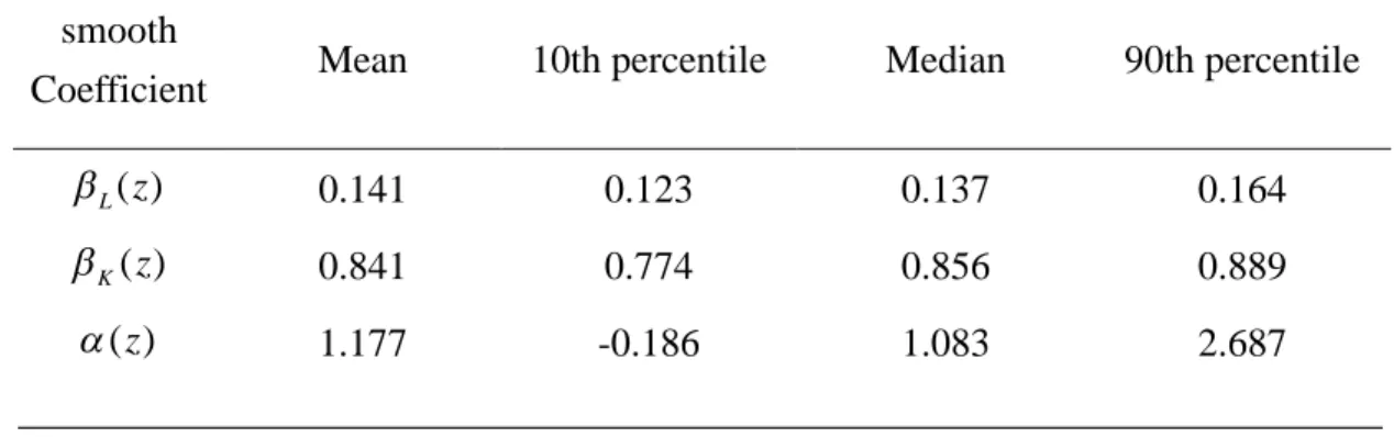
lnY_it   z_itz_it _klnK_it _LlnL_it  v_it u e_i  t T (3) Table 1 tabulates the mean values and the 10th, median, and 90th of the smooth coefficients estimates of our semiparametric model (2). Table 2 presents the parameter estimates of the Cobb-Douglas function.

The ML estimates (standard errors) of  and  of the SSCM are 2.3367 (0.0052) and 0.0217 (1.75 10 ), 6 respectively. As a result the implied estimates of

2

v

 and 2

u

 are 0.1225 and 0.0224, respectively. Evidence is found that the rate of the technical efficiency improvement () of the SSCM is faster than that of the Cobb-Douglas function. This indicates that the potentially restrictive Cobb-Douglas functional form may not be well descriptive of the true but unknown production technology, in such a way as to underestimate the evolution speed of the technical efficiency. In addition, the average technical efficiency score derived from the Cobb-Douglas function is as low as 0.431, which is much less than 0.714 of the SSCM. The left box of Figure 1 draws the residual distribution of (2), whereas the right box draws that of (3). The former distribution is seen to be somewhat higher than the latter distribution, due partially to the smaller inefficiency of (2) than that of (3). The figure shows that the middle 50% of the residuals yielded from (2) are less dispersed than those from (3). The SSCM outperforms the Cobb-Douglas model in

6

terms of the goodness of fit, since the R-squares of the SSCM and the Cobb-Douglas models are equal to 0.927 and 0.648, respectively.2

Table 1. Estimates of the Smooth Coefficient Functions

_____________________________________________________________________

Table 2. Parameter Estimates of the Cobb-Douglas Function

2

We also estimate a translog production function, in which the additional terms of _{(ln )L ,}2 _(lnK)2_,

and ln * lnL K are appended to (14). The estimated average technical efficiency score and

R-square are close to those of the Cobb-Douglas function.

smooth

Coefficient Mean 10th percentile Median 90th percentile ( ) L z  0.141 0.123 0.137 0.164 ( ) K z  0.841 0.774 0.856 0.889 ( )z  1.177 -0.186 1.083 2.687 Variables Parameter

Estimates Standard Errors Intercept 6.5087*** 0.30109 lnL 0.28062*** 0.01906 lnK 0.55787* 0.01034 z -0.04321*** 0.01178 2 z 0.01479*** 0.00167  _{0.00133*** 0.00043} 2 2 u v   1.26864*** 0.21348 2 2 2 u u v    0.98806*** 0.00211

V. Conclusions

This paper is devoted to extending the SSCM of Li et al. (2002) from a

cross-sectional framework to the more popular and important panel data framework, which allows for the presence of time-varying technical efficiency. Under the maintained framework, we develop the likelihood function for the composed errors, which cannot be directly estimated by the maximum likelihood due to the presence of nonparametric and smooth coefficient functions. We instead propose a group of estimation procedures adapting from Robinson (1988) and Fan et al. (1996), who develop valid estimation approaches for a semiparametric model. A local least squares method with a kernel weight function is suggested to estimate the smooth coefficient functions. Monte Carlo simulations are used to confirm that our proposed estimators of interest have the desirable property of consistency.

Due to the fact that the SSCM with error components is a quite flexible specification appropriate for describing a general production and/or cost regression relationship with varying coefficients and panel data are getting more important for applied researchers for the past two decades, our modeling offers an alternative and is perhaps preferable to a parametric model. Using international macroeconomic panel data the SSCM suggests that the marginal effects of labor and capital stock are

significantly affected by human capital nonlinearly. In addition, the slope of the estimated _L( )z is increasing after z = 6, while the shape of the estimated _K( )z is concave after z = 6. A parametric model fails to provide such information. The empirical study appears to support that the SSCM is preferable to the traditional Cobb-Douglas (translog) function in terms of the goodness of fit and the ability of Log-likelihood 1272.84

8

extracting valuable information from the data.

參考文獻

Aigner, D.J., C.A.K. Lovell, and P. Schmidt (1977), Formulation and estimation of stochastic frontier production function models, Journal of Econometrics, 6, 21-37.

Battest, G.E. and T.J. Coelli (1992), Frontier production functions, technical efficiency and panel data: With application to paddy farmers in India, Journal of Productivity Analysis, 3, 153-169.

Cai, Z., J. Fan, and R. Li (2000a), Efficient estimation and inferences for

varying-coefficient models, Journal of the American Statistical Association, 95, 888–902.

Cai, Z., J. Fan, and Q. Yao (2000b), Functional coefficient regression models for nonlinear time series models, Journal of the American Statistical Association, 95, 941–956.

Chen, R. and R.S. Tsay (1993), Functional –coefficient autoregressive models, Journal of the American Statistical Association, 88, 298-308.

Cheng, M.Y. and W. Zhang, (2007), Statistical estimation in generalized multiparameter likelihood models. Manuscript.

Cleveland, W. S., E. Grosse, and W. M. Shyu, (1991), Local regression models, in Statistical Models in S (Chambers, J. M. and T. J. Hastie, eds), 309–376, Wadsworth & Brooks, Pacific Grove.

Duffy, J. and C. Papageorgiou, (2000), A cross-country empirical investigation of the aggregate production function specification, Journal of Economic Growth, 5, 87–120.

Fan, J. (1992), Design-adaptive nonparametric regression. Journal of the American Statistical Association, 87, 998–1004.

Fan, Y., Q. Li, and A. Weersink (1996), Semiparametric estimation of stochastic production frontier models, Journal of Business and Economic Statistics, 14, 460-468.

Fan, J. and W. Zhang (1999), Statistical estimation in varying-coefficient models, The Annals of Statistics, 27, 1491–1518.

Fan, J. and W. Zhang (2008), Statistical methods with varying coefficient models, Statistics and Its Interface, 1, 179-195.

Hastie, T. and R. Tibshirani (1993), Varying coefficient models, Journal of the Royal Statistical Society, Series B, 55, 757-796.

Hoover, D. R., J. A. Rice, C. O. Wu, and L.P. Yang (1998), Nonparametric smoothing estimates of time-varying coefficient models with longitudinal data, Biometrika, 85, 809–822.

Kauermann, G. and G. Tutz (1999), On model diagnostics using varying coefficient models, Biometrika, 86, 119–128.

Kneller, R. and A. Stevens (2003), The specification of the aggregate production function in the presence of inefficiency, Economics Letters, 81, 223–226.

Kumbhakar, S.C. (1990), Production frontiers, panel data, and time-varying technical inefficiency, Journal of Econometrics, 46, 201-212.

Li, Q., C.J. Huang, D. Li, and T.T. Fu (2002), Semiparametric smooth coefficient models, Journal of Business and Economic Statistics, 20, 412–422.

Meeusen, W. and van den Broeck (1977), Efficiency estimation from Cobb-Douglas production functions with composed error, International Economic Review, 18, 435-444.

Robinson, P.M. (1988), Root-N-Consistent semiparametric regression, Econometrica, 56, 931-54.

Stock, J.H. (1989), Nonparametric policy analysis, Journal of the American Statistical Association, 84, 567-575.

Wu, C. O., C. T. Chiang, and D. R. Hoover (1998), Asymptotic confidence regions for kernel smoothing of a varying-coefficient model with longitudinal data. Journal American Statistical Association, 93, 1388–1402.

10 計畫成果自評 本研究案於計畫申請時，係以三年期計畫為藍本進行規劃，打算用三年時 間，逐步探討平滑係數與分量迴歸縱橫資料模型。唯經過評審後被刪成一年期計 畫，時間縮短的結果，只能完成第一部分，故本結案報告內容僅為以平滑係數縱 橫資料模型為主，探討估計生產效率的方法。 本研究成果，主要將平滑係數迴歸模型從橫斷面擴充至縱橫資料模型，並容 許生產無效率項隨時間變動，更符合實際情況。使用 Monte Carlo 模擬方法，證 明本研究建議的估計步驟，可以得到具備一致性的係數估計式，適合用於實證分 析，提供實證研究者更多的選擇，故應有一定的學術價值。