前饋式零相位誤差強健控制器應用於微型化藍光讀寫頭兩段式致動器設計

國 立 交 通 大 學

機械工程學系

碩 士 論 文

前饋式零相位誤差強健控制器應用於微型化藍

光讀寫頭兩段式致動器設計

Dual-Stage Actuator Feed-forward Robust Controller Design

with ZPETC Method In Miniaturized Optical Disc Drive

指導教授：鄭泗東 教授

研 究 生：周伯謙

Dual Stage Actuator Feed-forward Robust Controller Design

with ZPETC Method In Miniaturized Optical Disc Drive

前饋式零相位誤差強健控制器應用於微型化藍

光讀寫頭兩段式致動器設計

研 究 生：周伯謙 Student : Po-chien Chou

指導教授：鄭泗東教授 Advisor : Dr. Stone Cheng

國 立 交 通 大 學

機械工程學系

碩 士 論 文

Department of Mechanical Engineering,

National Chiao-Tung University,

June 2008

Hsinchu , Taiwan, Republic of China

i

摘要

有PZT的雙軸控制致動器設計用來提供高速尋軌與聚焦的讀取動

作,解決以往微型化讀寫頭(mini-ODD)容易受外在干擾影響而不易

快速讀取資料情況,新式的蹺板式雙軸致動器機械上有點對於聚焦

能提供更迅速更精確的讀取.主致動器VCM做大範圍的低頻調整移

動聚焦尋軌,同時配合PZT精密小範圍高頻的精密調整.遠比傳統單

軸VCM來的迅速.在機構的伺服控制方面,期望微型化藍光光學讀寫

頭在10800rpm高速運轉下,控制系統一方面能達到高速響應,另一方

面對於低頻與高頻的干擾能有效排除,現今雙軸伺服控制設計更比

起傳統單軸致動器控制器的設計更顯得困難與複雜,再建模基礎下,

建立一個有效的強健干擾觀察迴路對致動器做控制,一方面強健傳

統PID控制器對於干擾影響的不穩定性,一方面抑制建模過程中系統

不確定因素所帶來的影響.對於突發干擾能做有效抑制.解決微型讀

寫頭受外在衝擊時對系統讀取碟片所帶來的影響.另外對於PZT壓電

效應與碟盤偏心不平整所產生的週期性干擾,以快速零相位誤差控

制迴路(ZPET-FF)控制迴路對其做修正,以強健觀察迴路系統抑制突

發干擾,以快速零相位誤差控制迴路抑制週期性干擾,在兩者搭配下

期望能更快速的達到系統的預估的頻率響應值是本論文的目的

ii

Abstract

A swing-arm/PZT dual-stage actuator is designed to provide high

performance solution to realize precise tracking and focusing operation of

miniaturized optical disc drive (mini-ODD). Because of its dual-stage

mechanical characteristics can perform the focusing action smoother and

more precise; the servo system to control such a dual-stage system tends

to be more complex than a conventional single-stage ODD system. Based

on the modeling results, a robust tracking observer control system with

both two degree of freedom control system is proposed. In order to

suppress the disturbance quickly, this paper designs the zero phase error

tracking controller (ZPETC) plus feed-forward servo loop with the

memory of tracking error to satisfy tracking error transient response and

improve the sensitive focusing performance of dual-stage miniaturized

actuator. The conclusion points out that the proposed robust ZPETC

servo system has a precise tracking response and rejects both periodic

disturbance and sudden disturbance.

iii

誌謝

感謝指導老師鄭泗東教授這兩年來對我的諄諄教誨與細心指導,使我不僅再分 析邏輯的能力有所提升,並且完成本篇論文研究.期間鄭泗東教授的鼎力相助以 及支持鼓勵,使控制實驗可以順利成功,學生我點滴在心頭,由衷感激鄭老師的協 助與打氣!也感謝林君穎學長與侯冠州學長提供光學頭組裝的設備與量測的空間, 以及對我的關心與鼓勵,在施錫富教授熱心的指導之下,使我對於光陸方面的組 裝有著顯著的進步,更謝謝鄭泗東老師與吳炳飛老師使我對控制構思與干擾阻絕 研究方向的思考判斷技巧有著顯著的進步,使的我論文能更臻完整.此外感謝呂 宗熙實驗室學長對於系統健模的幫忙與建議,讓我在實驗方法與思考方向有更大 的突破,在此也謝謝曹致維,余偉廷,郭富存等等好同學提供寶貴建議!同時,感謝 實驗室學長以及學弟的支持與鼓勵,讓我能夠再碩士求學生涯中留下快樂的回憶 感謝交大電機控制工程研究所,中興機械工程研究所,交大光電研究所,經濟 部微型化光學頭計畫,以及行政院國家科學委員會提供本研究所需的經費,使得 言就可以順利的進行 最後,僅將本論文獻給一路走來永遠支持我的家人,謝謝你們對我的關心與 照顧,使我能夠堅持到底地完成學業,並且打開雙臂迎接嶄新的挑戰

iv

Table of Conents

中文摘要 i ABSTRACT ii 誌謝 iii TABLE OF CONTENTS iv LIST OF FIGURES v 1. INTRODUCTION 1.1 Background ……….……... 1

1.2 Blue ray optical head ……… 3

2. ROBUST DISTURBANCE OBSERVER ON 2DOF SERVO SYSTEM 2.1 Tracking control system………... 7

2.2 Robust feedback controller based on disturbance observer……… . 8

2.3 Robust stability condition……… . 10

2.4 2DOF control System………. 13

3. ZERO PHASE ERROR TRACKING CONTROL AND SYSTEM IDENTIFICATION 3.1 Feed-forward control system……… 17

3.2 Phase pre-compensator design………. 18

3.3 ZPETC controller………. 19

3.4 System Identification……… 22

3.5 Least squares method……… 25

3.6 ARMAX model………. 26

4. TWO DEGREE OF FREEDOM IN DUAL-STAGE SERVO SYSTEM 4.1 Dual-stage control loop……….. 31

v

4.2 Two degree of freedom control ..……… 34

5. HIGH SPEED PERIODIC DISTURBANCE REJECTION USING ZPET-FF CONTROL 5.1 ZPET-FF loop………. 38

5.2 Estimators of VCM and PZT……… 39

6. EXPERIMENT AND SIMULATION 6.1 Seesaw frequency response and PZT frequency response……… 41

6.2 Piezoelectric ceramic ………... 43

6.3 System identification……… 45

6.4 2DOF system response……….... 48

6.5 Periodic disturbance response……….. 49

6.6 sudden disturbance reject……… 50

7. CONCLUSION………... ……….. 52

vi

FIGURE CAPTIONS

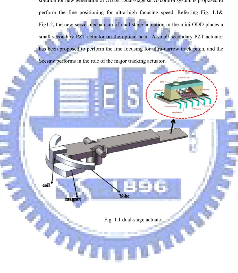
Fig. 1.1 dual-stage actuator ………...4

Fig. 1.2 dual-stage actuator action……….5

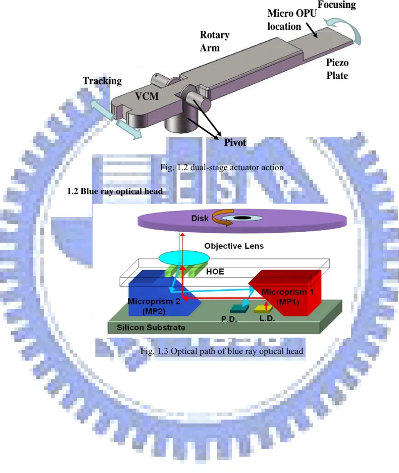
Fig. 1.3 Optical path of blue ray optical head………5

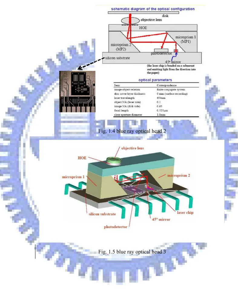
Fig. 1.4 blue ray optical head 2………..6

Fig. 1.5 blue ray optical head 3 ……….6

Fig. 1.6 optical head on seesaw actuator ………...7

Fig. 2.1 tracking servo system for ODD ………...9

Fig. 2.2 Robust feedback controller based on disturbance observer ………..10

Fig. 2.3 multiple perturbation of inner loop………12

Fig. 2.4 robust stability condition………13

Fig. 2.5 General model of 2DOF control System………16

Fig. 2.6 2DOF Control System……….16

Fig. 2.7.sudden disturbance model………...17

Fig. 2.8.step response………...18

Fig. 3.1 feed-forward control system………...20

Fig. 3.2 Feed-Forward (FF) controller……….21

Fig. 3.3 Feed-forward controller design………...…21

Fig. 3.4 Feed-forward controller………..22

Fig. 3.5 ZPETC controller ………...23

Fig. 3.6 ZPECT controller………24

Fig. 3.7 dynamical model……….26

vii

Fig. 3.9 input signals………27

Fig. 3.10 parametric model………..28

Fig. 4.1 Two-input-two-output control………35

Fig. 4.2 Two-input-one-output control………35

Fig. 4.3 dual-stage control loop………35

Fig. 4.4 two degree of freedom control………37

Fig. 4.5 action in initial time………38

Fig. 4.6 action in infinite time………..38

Fig. 5.1 ZPET-FF controller model………..40

Fig. 5.2 ZPET-FF loop……….40

Fig. 6.1 Seesaw frequency response……….…44

Fig. 6.2 PZT frequency response……….44

Fig. 6.3 piezoelectric ceramic………...45

Fig.6.4 piezoelectric ceramic………45

Fig. 6.5 System Identification of VCM………47

Fig. 6.6 System Identification of PZT………..47

Fig. 6.7 System Identification of VCM………49

Fig. 6.8 System Identification of PZT………..49

Fig. 6.9 servo system response……….50

Fig. 6.10 periodic disturbance response………..……….51

Fig. 6.11 sudden disturbance rejection………52

1

INTRODUCTION

1.1 Background

Optical disk drive is one of the most popular systems of information storage. Two promising candidates are near-field recording and holography. Holographic data storage technology provides far-field optical recording and readout. High capacities are obtained by using a very high numerical aperture optical stylus for reading data from and writing data onto the optical disk [4]. In optical holography, data are impressed onto an optical coherent beam using a spatial light modulator. Resulting in very small spot sizes approaching dimensions less than 100 nm, the focusing spot is near to the optical lens, requiring close proximity between the optical head and disk, making removability of the media more difficult. Referring Fig.1, the new servo mechanism of dual stage actuation in the mini-ODD places a small secondary PZT actuator on the optical head. The PZT actuator has been proposed to perform the fine focusing for narrow track pitch, and the Seesaw performs in the role of the major tracking actuator. Optical disk drive is one of the most popular systems of information storage. Two promising candidates are near-field recording and holography. Holographic data storage technology provides far-field optical recording and readout. High capacities are obtained by using a very high numerical aperture optical stylus for reading data from and writing data onto the optical disk [4]. In optical holography, data are impressed onto an optical coherent beam using a spatial light modulator. Resulting in very small spot sizes approaching dimensions less than 100 nm, the focusing spot is near to the optical lens, requiring close proximity between the optical head and disk, making removability of the media more difficult. From the control point view, it cannot be achieved by the current ODDs employing the sole actuator of VCM. The VCM limits the bandwidth extension in the single-stage servo system because of its mechanical resonances and

2

high frequency uncertainties [3]. As such dual-stage actuation is seen to be the solution for new generation of ODDs. Dual-stage servo control system is proposed to perform the fine positioning for ultra-high focusing speed. Referring Fig. 1.1& Fig1.2, the new servo mechanism of dual stage actuation in the mini-ODD places a small secondary PZT actuator on the optical head. A small secondary PZT actuator has been proposed to perform the fine focusing for ultra-narrow track pitch, and the Seesaw performs in the role of the major tracking actuator.

3

Micro OPU

location

Focusing

Tracking

Piezo

Plate

Pivot

Rotary

Arm

VCM

Micro OPU

location

Focusing

Tracking

Piezo

Plate

Pivot

Rotary

Arm

VCM

Fig. 1.2 dual-stage actuator action 1.2 Blue ray optical head

4

Fig. 1.4 blue ray optical head 2

5

Fig. 1.6 optical head on seesaw actuator

There are two methods to improve the optical devices to exceed our hope. One method is improving the gain margin by analysis and redesign of VCM parameters [10]. It regulates the topology optimization and shape optimization of VCM. The VCM suspension design is to decrease the shock resistances and the equivalent mass with increasing first torsion frequency. The shape design is mass reduction for reducing power consumption [7] [9], and the position error signal (PES) would be maintained in minimum. Because of mini VCM structure and complex magnetic circuit, this mechanical design has some problems to decrease it thickness [10]. The complexity will not only impact the cost of the ODD but also degrade the servo performance owing to long delay time. A control problem is that the overshoot or oscillation may delay of the output signal and result in a long seeking time.

The other method is accomplished by control designed for robust performance [3]. The system must follow the track to keep the residual focusing error below its tolerance. Hence, the focusing servo system should keep the robust performance against sudden disturbance. Generally, the conventional tracking servo system is

6

accomplished by the feedback servo designed using PID control. It is difficult to compensate the sudden disturbance and periodic disturbance. The robust control and the adaptive control methods are used to eliminate the effects of uncertainty for systems with uncertainty. The adaptive control method has more applications in industrial and the robust control can effectively control systems with parameter uncertainty [7]. Recently, the several robust control has been realized by H∞ control theory, disturbance observer and so on. The robust control system based on H∞ control theory can keep a robust stable condition for parameter variation by its loop shaping [8] [9]. This paper focuses on a useful control loop, a two degree of freedom servo system is designed on the basis of doubly coprime factorization to consider the robust stability [8].

This paper is organized as follows. Section II used the robust tracking observer control system based on both two degree of freedom control system. Section III discusses the zero phase error tracking control (ZPETC) and a method of the system identification. Section IV gives a brief introduction on dual-stage servo system. Section V the new control method of ZPETC loop is in the dual stage robust control system. The performance of the proposed control scheme and experimental results are discussed in Section V. The conclusion is discussed in Section VI.

7

II. ROBUST DISTURBANCE OBSERVER ON

2DOF SERVO SYSTEM

2.1 Tracking control system

Significant progress in areal storage density of an ODD can be accomplished by using a dual-stage actuator system. In such a servo system a high-bandwidth and highly accurate micro actuator is used in combination with a traditional VCM to position the read/write head over the data track. The track following servo control system is required to perform robustly in the presence of uncertainties induced by disturbances and product variability. Because of the conventional is difficult to carry out the quick suppression of the sudden disturbance. The proposed two degree of freedom servo system considering the robust stability according to inertia variation is designed on the basis of Doubly Coprime Factorization and Disturbance Observer. For the design of a robust servo system, uncertainties are taken into account in the form of an uncertainty model. The uncertainty model consists of a nominal model together with an unknown but bounded description of the disturbances and uncertainty.

Fig. 2.1 tracking servo system for ODD

Generally, the block diagram of the tracking control system for an optical disk drive is shown in Fig2.1. Here, P(s) is the tracking actuator for an optical disk drive, which is a moving-coil actuator. xref is the tracking position reference to be followed.

8

2.2 Robust feedback controller based on disturbance observer

Based on coprime factorization, the transfer function P(s) of the tracking actuator VCM and PZT are expressing by:

( ) ( ) ( ) N s P s D s = (1)

Bezout identity equation : ( )N s X s⋅ ( )+D s Y s( ) ( ) 1⋅ = (2) The robust feedback controller C(s) is determined by the coprime factorization

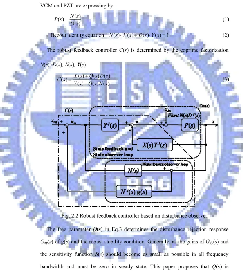
N(s), D(s), X(s), Y(s). ( ) ( ) ( ) ( ) ( ) ( ) ( ) X s Q s D s C s Y s Q s N s + = − (3)

Fig. 2.2 Robust feedback controller based on disturbance observer

The free parameter Q(s) in Eq.3 determines the disturbance rejection response

Gdy(s) of g(s) and the robust stability condition. Generally, as the gains of Gdy(s) and

the sensitivity function S(s) should become as small as possible in all frequency bandwidth and must be zero in steady state. This paper proposes that Q(s) is determined by the stable and proper function g(s). A gain of g(s) is unity in steady state. The sensitivity function S(s) and the disturbance rejection response Gdy(s) are

9

represented as shown in (6) and (7). The block diagram of proposed robust control system is illustrated as shown in Fig. 2.2.

( ) ( ) ( ), (0) 1 ( ) Y s Q s g s g N s = ⋅ = (4)

(

)

( ) ( ) ( ) ( ) ( ) ( ) ( ) ( ) ( ) ( ) ( ) ( ) 1 ( ) X s Q s D s X s g s C s Y s Q s N s Y s N s Y s g s + ⋅ = = + − ⋅ ⋅ ⋅ − (5)

[

]

Sesitivity function ( )S s =D s Y s( )⋅ ( ) 1⋅ −g s( ) (6)

[

]

Disturbance rejection response G sdy( )=N s Y s( )⋅ ( ) 1⋅ −g s( ) (7)

Proof: 1 ( ) ( ) ( ) : ( ) ( ) ( ) 1 ( ) 1 ( ) ( ) ( ) in in dis P s P s G s x u x Y s X s X s P s P s Y s Y s = ⋅ ⋅ + ⎛ ⎞ ⎛ ⎞ +_⎜ ⋅ _⎟ +_⎜ ⋅ _⎟ ⎝ ⎠ ⎝ ⎠ ( ) ( ) ( ) ( ) ( ) ( ) in ( ) ( ) ( ) dis P s Y s P s x u x Y s X s P s Y s X s P s ⎡ ⎤ ⎡ ⋅ ⎤ =_{⎢ ⎥}⋅ +_{⎢ ⎥}⋅ + ⋅ + ⋅ ⎣ ⎦ ⎣ ⎦

[

]

( ) 1 1 ( ) ( ) ( ) 1 ( ) 1 ( ) ( ) in ref in in ref g s g s u x N s u x u x x N s g s g s N s = + ⋅ ⋅ − ⇒ = ⋅ − ⋅ ⋅ − − ( ) 1 1 ( ) ( ) ( ) ( ) ( ) ( ) 1 ( ) ref 1 ( ) ( ) ( ) ( ) ( ) dis P s g s Y s P s x x x x Y s X s P s g s g s N s Y s X s P s ⎡ ⎤ ⎡ ⎤ ⎡ ⋅ ⎤ =_{⎢ ⎥ ⎢}⋅ ⋅ − ⋅ ⋅ _{⎥ ⎢}+ _⎥⋅ + ⋅ − − + ⋅ ⎣ ⎦ ⎣ ⎦ ⎣ ⎦

(

)

(

)

(

)

( ) ( ) ( ) ( ) 1 ( ) ( ) ( ) ( ) 1 ( ) ( ) ( ) 1 ( ) ( ) ( ) ref dis N s P s x N s Y s g s P s x x N s Y s g s N s X s g s g s P s ⋅ ⋅ + ⋅ ⋅ − ⋅ ⋅ = ⋅ ⋅ − +⎡_⎣ ⋅ ⋅ − + ⎤_⎦⋅

[

]

[

]

[

]

[

]

[

]

( ) ( ) ( ) ( ) ( ) ( ) ( ) ( ) 1 ( ) ( ) ( ) 1 ( ) ( ) ( ) 1 ( ) ( ) ( ) _{( ) ( )} 1 ( ) 1 ( ) ( ) ( ) 1 ( ) ( ) ( ) 1 ( ) ref ref dis dis N s P s x N s P s x P s x P s x N s Y s g s N s Y s g s x N s X s g s g s P s _{X s g s} P s Y s N s Y s g s N s Y s g s ⋅ ⋅ ⋅ ⋅ + ⋅ + ⋅ ⋅ ⋅ − ⋅ ⋅ − = = ⎡ ⋅ ⋅ − + ⎤⋅ ⎡ ⎤ ⎣ ⎦ _{+ + ⋅} + _{⎢ ⎥} ⋅ ⋅ − ⋅ ⋅ − _{⎣ ⎦}

[

]

[

]

[

]

[

]

[

]

( ) ( ) ( ) ( ) ( ) 1 ( ) ( ) ( ) ( ) ( ) 1 ( ) ( ) ( ) ( ) 1 ( ) ( ) ( ) ( ) ( ) ( ) ( ) 1 1 ( ) ( ) ( ) 1 ( ) ( ) ( ) ( ) ( ) ( ) 1 ( ) ref ref dis dis N s N s x N s x N s Y s g s x N s D s _x N s Y s g s D s D s Y s g s x X s g s N s N s X s g s Y s N s Y s g s D s D s Y s D s Y s g s ⋅ ⋅ _{⋅ + ⋅ ⋅ − ⋅} + ⋅ ⋅ ⋅ − ⋅ ⋅ − = = ⎡ ⎤ ⎡ ⋅ ⎤ +_⎢ + _⎥⋅ +_⎢ + _⎥ ⋅ ⋅ − ⋅ ⋅ ⋅ − ⎣ ⎦ ⎣ ⎦

[

]

[

]

[

]

[

]

[

]

( ) ( ) ( ) 1 ( ) ( ) ( ) 1 ( ) 1 ( ) ( ) 1 ( ) ( ) ( ) 1 ( ) ( ) ( ) ( ) 1 ( ) ref dis N s x N s Y s g s x D s Y s g s x D s Y s g s N s X s g s g s D s Y s g s ⋅ + ⋅ ⋅ − ⋅ ⋅ ⋅ − = ⎡ ⎤ ⋅_⎣ ⋅ ⋅ − + ⋅ ⋅ − + _⎦ ⋅ ⋅ −

10

[

]

( ) ( ) ( ) 1

_[

[

_]

( )

]

( ) ( ) 1 ( ) ( ) ( ) 1 ( ) ref dis N s x N s Y s g s x x D s Y s g s D s Y s g s ⋅ + ⋅ ⋅ − ⋅ ⎡ ⎤ =_⎣ ⋅ ⋅ − _⎦⋅ ⋅ ⋅ −

2.3 Robust stability condition

The inner loop is the closed loop system based on the state feedback and the state observer. The outer loop system is equivalent to the closed loop system based on disturbance observer. Fig. 2.2 points out that g(s) is equivalent to the low pass filter of the conventional disturbance observer and defines the complementary sensitivity function T(s) of the outer loop system. [1−g(s)] is the sensitivity function of the outer

loop system, and [N(s)·Y(s)] is the sensitivity function of the inner loop.

Fig. 2.3 multiple perturbation of inner loop

Since the lower resonant frequency is dominant for the frequency characteristics of the tracking actuator, we use the following approximation:

2 ˆ( ) a s K P s M s D s K = ⋅ + ⋅ +

Ka , M , D and Ks are the force constant, the mass of the moving parts of the

actuator, and the viscosity coefficient and the spring modulus. We denote P(s) as

ˆ( )

P s

when these parameters are nominal. Taking multiplicative perturbation E(s) into account, the model is given by:

[

]

ˆ

( ) ( ) 1 ( )

11

Fig. 2.4 robust stability condition

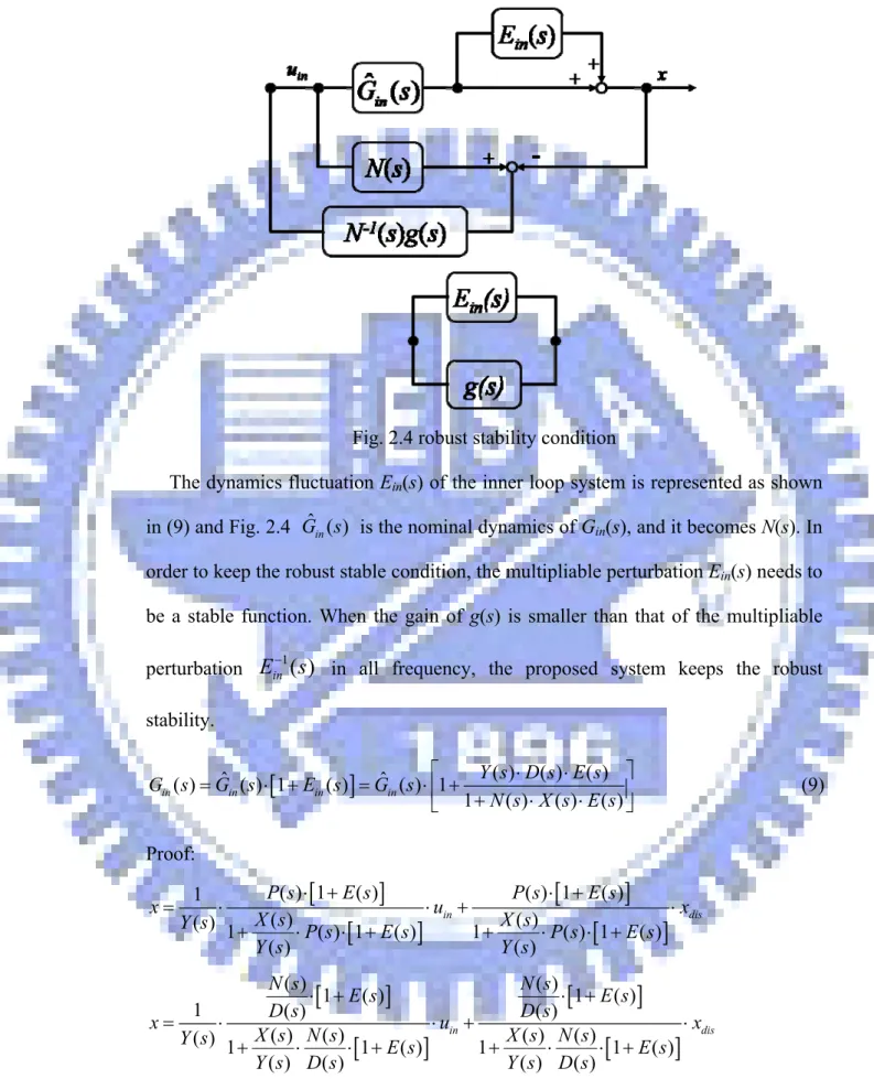
The dynamics fluctuation Ein(s) of the inner loop system is represented as shown

in (9) and Fig. 2.4 is the nominal dynamics of Gin(s), and it becomes N(s). In

order to keep the robust stable condition, the multipliable perturbation Ein(s) needs to

be a stable function. When the gain of g(s) is smaller than that of the multipliable perturbation

E

_in−1

( )

s

in all frequency, the proposed system keeps the robust stability.

[

]

( ) ( ) ( ) ˆ ˆ ( ) ( ) 1 ( ) ( ) 1 1 ( ) ( ) ( ) in in in in Y s D s E s G s G s E s G s N s X s E s ⎡ ⋅ ⋅ ⎤ = ⋅ + = ⋅ +_{⎢ ⎥} + ⋅ ⋅ ⎣ ⎦ (9) Proof:

[

]

[

]

[

]

[

]

( ) 1 ( ) ( ) 1 ( ) 1 ( ) ( ) ( ) 1 ( ) 1 ( ) 1 ( ) 1 ( ) ( ) ( ) in dis P s E s P s E s x u x X s X s Y s _{P s E s P s E s} Y s Y s ⋅ + ⋅ + = ⋅ ⋅ + ⋅ + ⋅ ⋅ + + ⋅ ⋅ +

[

]

[

]

[

]

[

]

( ) ( ) 1 ( ) 1 ( ) 1 ( ) ( ) ( ) ( ) ( ) ( ) ( ) 1 1 ( ) 1 1 ( ) ( ) ( ) ( ) ( ) in dis N s N s E s E s D s D s x u x X s N s X s N s Y s _{E s E s} Y s D s Y s D s ⋅ + ⋅ + = ⋅ ⋅ + ⋅ + ⋅ ⋅ + + ⋅ ⋅ + ˆ ( )_in G s

12

[

]

[

]

[

]

( ) 1 ( ) ( ) ( ) 1 ( ) ( ) ( ) ( ) ( ) 1 ( ) in dis N s E s u N s Y s E s x x D s Y s N s X s E s ⋅ + ⋅ + ⋅ ⋅ + ⋅ = ⋅ + ⋅ ⋅ +

[

]

[

]

( ) 1 ( ) ( ) ( ) 1 ( ) 1 ( ) ( ) ( ) in dis N s E s u N s Y s E s x x N s X s E s ⋅ + ⋅ + ⋅ ⋅ + ⋅ = + ⋅ ⋅

[

]

1 ( ) ˆ ( ) ( ) 1 ( ) ( ) ( ) in in dis E s x G s u Y s x N s X s E s + = ⋅ ⋅ + ⋅ + ⋅ ⋅

[

]

_[

_]

1 ( ) ( ) ( ) ( ) ( ) ˆ ( ) ( ) 1 ( ) ( ) ( ) in in dis N s X s Y s D s E s x G s u Y s x N s X s E s ⎧ + ⋅ + ⋅ ⋅ ⎫ = ⋅_{⎨ ⎬}⋅ + ⋅ + ⋅ ⋅ ⎩ ⎭

[

]

( ) ( ) ( ) ˆ ( ) 1 ( ) 1 ( ) ( ) ( ) in in dis Y s D s E s x G s u Y s x N s X s E s ⎧ ⋅ ⋅ ⎫ = ⋅ +_{⎨ ⎬}⋅ + ⋅ + ⋅ ⋅ ⎩ ⎭

For the purpose of satisfying the robust stability condition (9) and stabilizing the

Ein(s), this paper suitably designs g(s), the gains of state feedback and state observer.

( ) ( ) 1 in E s g s⋅ _∞ < (10) Proof:

{

_ˆ

}

( ) ( ) ( ) (1 ( )) ( ) in in in in g s N s u G s E s u N s ⎡ ⎤ ⋅ −_⎣ ⋅ + _⎦⋅ ⋅

[

]

{

}

( ) ( ) ( ) (1 ( )) ( ) ( ) ( ) in in in in g s N s u N s E s u E s g s N s ⋅ − ⋅ + ⋅ ⋅ = − ⋅

Moreover, as the robust control system is requested to keep the desired disturbance rejection response Gdy(s), the proposed system should consider the

perturbation of Gdy(s) caused by the parameter variation. The dynamical model of

disturbance input signal is xdis(s). Moreover, the position disturbance xpd(s) caused by

xdis(s) can he defined as shown in Eq11. Hence, the disturbance suppression response

Gdy(s) of tested servo system is determined by Eq.12.

2 ( ) a ( ) pd dis s K x s x s M s D s K = ⋅ ⋅ + ⋅ + (11)

[

]

( ) ( ) ( ) ( ) 1 ( ) ( ) dy pd x s G s D s Y s g s x s = = ⋅ ⋅ − (12) Proof:

13 ( ) ( ) ( ) ( ) ( ) ( ) pd dis dis N s x s P s x s x s D s = ⋅ = ⋅

[

]

[

]

( ) ( ) ( ) ( ) 1 ( ) ( ) ( ) ( ) 1 ( ) ( ) ( ) pd dis N s x s D s Y s g s x s D s Y s g s x s D s = ⋅ ⋅ − ⋅ = ⋅ ⋅ − ⋅ ⋅

[

]

( ) ( ) ( ) ( ) 1 ( ) ( ) is equal to Eq.7 dy dis G s x s =N s Y s⋅ ⋅ −g s ⋅x s 144424443

The tested robust feedback controller C(s) keeps both the desired robust stable condition for parameter variations and the desired disturbance suppression response. In order to realize these robust control performances of C(s), this paper satisfies the both equations Eq.13. ε is the gain margin of the disturbance suppression response. When ε is small, the tested robust feedback controller C(s) has a disturbance suppression response. In this paper, the feedback controller C(s) satisfies

both the robust stability condition on ± 20% multiplicative perturbation of spring constant Ks, and the sensitivity function S(s) becomes -60dB around 100[rad/sec].

Therefore, the gain margin ε is 0.01, and the poles of tested robust feedback controller C(s) are determined as shown in system ID.

( ) ( ) pd x s S s⋅ _∞ <ε (13)

[

]

{

}

( ) ( ) ( ) 1 ( ) pd x s D s Y s g s ε ∞ ⋅ ⋅ ⋅ − < 1 1−g s( ) < ⋅ε ⎡_⎣D s Y s x( )⋅ ( )⋅ _pd( )s ⎤_⎦ − 2.4 2DOF control System

The robust control system based on disturbance observer has sometimes a high overshoot and an oscillated response. In order to overcome these problems, this paper proposes a new two-degrees-of-freedom control system based on doubly coprime factorization.

14

Fig. 2.5 General model of 2DOF control System

Fig. 2.6 2DOF Control System

Where, P(s) denotes the plant to be controlled. The feedback compensator C1(s)

defines both the disturbance rejection response Gdy(s) and a robust stability. The

feed-forward compensator C2(s) defines a reference input response Gry(s). It is

obvious that the feed-forward compensator C2(s) is not able to improve the stability

of the closed-loop system. Therefore, the feedback controller C1(s) must be designed

to stabilize the feedback system composed of P(s) and C1(s).

[

]

( ) ( ) ( ) 1 ( ) dy G s =N s Y s⋅ ⋅ −g s ( ) ( ) ( ) ry G s =N s R s⋅

[

]

( ) ( ) ( ) 1 ( ) S s =D s Y s⋅ ⋅ −g s

15 Proof: ( ) ( ) 1 ( ) ( ) ( ) : ( ) ( ) ( ) ( ) ( ) 1 1 ( ) ( ) ( ) ( ) in in dis N s N s D s D s G s x u x Y s X s N s X s N s Y s D s Y s D s = ⋅ ⋅ + ⎛ ⎞ ⎛ ⎞ +_⎜ ⋅ _⎟ +_⎜ ⋅ _⎟ ⎝ ⎠ ⎝ ⎠ ( ) _in ( ) ( ) _dis x N s u= ⋅ +N s Y s x⋅ ⋅

[

]

( ) ( ) 1 ( ) ( ) ( ) ( ) 1 ( ) 1 ( ) ( ) in ref in in ref g s R s g s u R s x N s u x u x x N s g s g s N s = ⋅ + ⋅ ⋅ − ⇒ = ⋅ − ⋅ ⋅ − − ( ) 1 ( ) ( ) ( ) ( ) 1 ( ) ref 1 ( ) ( ) dis R s g s x N s x x N s Y s x g s g s N s ⎡ ⎤ = ⋅_⎢ ⋅ − ⋅ ⋅ _⎥+ ⋅ ⋅ − − ⎣ ⎦

[

]

( ) ( ) ref ( ) ( ) 1 ( ) dis x N s R s x= ⋅ ⋅ +N s Y s⋅ ⋅ −g s ⋅x

[

]

2( ) ( ) ( ) 1( ) ( ) ( ) 1 C s =D s R s⋅ +C s ⋅ N s R s⋅ − Proof:

[

1 2

]

[

1 2

]

1 1 ( ) ( ) ( ) ( ) ( ) ( ) ( ) ( ) 1 ( ) ( ) ( ) ( ) ( )

ref ref ref

C s C s P s C s C s N s N s R s x x x C s P s D s C s N s + ⋅ + ⋅ ⋅ ⋅ = ⋅ = ⋅ + ⋅ + ⋅

[

1 2

]

1 ( ) ( ) ( ) ( ) ( ) ( ) ref ref C s C s R s x x D s C s N s + ⋅ = + ⋅

[

D s R s( )⋅ ( )+C s N s R s1( )⋅ ( )⋅ ( )

]

⋅xref =

[

C s1( )+C s2( )

]

⋅xref

[

]

2( ) ( ) ( ) 1( ) ( ) ( ) 1 C s =D s R s⋅ +C s ⋅ N s R s⋅ −

16

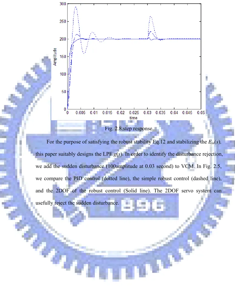
Fig. 2.8.step response

For the purpose of satisfying the robust stability Eq.12 and stabilizing the Ein(s),

this paper suitably designs the LPF g(s). In order to identify the disturbance rejection, we add the sudden disturbance (100amplitude at 0.03 second) to VCM. In Fig. 2.5, we compare the PID control (dotted line), the simple robust control (dashed line), and the 2DOF of the robust control (Solid line). The 2DOF servo system can usefully reject the sudden disturbance.

17

III ZERO PHASE ERROR TRACKING

CONTROL AND SYSTEM

IDENTIFICATION

3.1 feed-forward control system

A control problem is that the overshoot or oscillation may delay of the output signal and result in a long seeking time. Solving this problem can use the ZPET Controller to repair the phase error and delay. The ZPETC design method was proposed by Tomizuka [10] to improve tracking accuracy in feedback control loop. The design of the ZPETC controller directly cancels the stable (well – damped) poles and zeros in the position feedback loop and compensates for the unstable zeros to achieve the zero phase error in the servo system [4]. Recently, the Miniaturized Optical Disc Drive has been realized by ZPET control system. This is a new developed methods involve compensation for all undesired zeros or heavy computations [2] [3]. This system has been shown to reduce residual focusing error far better than conventional feedback control, and has demonstrated the capability to reduce the residual focusing error [5]. The feed-forward controller desires to track any time varying output signal without the phase error. Those uncertain item and delay time produce the phase error. Although it is further assumed that a feedback controller remains system stable, the feed-forward controller is useful to achieve a good tracking performance fast.

In the past, this pole-zero cancellation method was not approach to stable to any condition. If there exist non-minimum phase zeros in the transfer function to be controlled, this method is no doubt make the actuator unstable. The pole-zero cancellation method only cancels those stable zeros and poles, but the system still have phase lag between the actual output signal and the desired tracking signal.

18

Tomizuka (1987) solved this control problem from the frequency response and designed a new type of feed-forward controller. The proposed feed-forward control system can reduce the tracking error caused by time delay.

Fig. 3.1 feed-forward control system

It supposes the feedback closed loop transfer function in the discrete time. The transfer function includes the stable plant (actuator) and feedback controller. Referring Fig.3.1 the transfer function write down as:

( ) ( )

( ) ( )

( )

1 function denominator function numerator 1 1 1 1 1 1 _{( )} ( ) 1 c d c closed C A z z P z z B z G z C z P z − − − − − − − − ⋅ ⋅ ⋅ = = + 64748 123 (14) Where 1 1 2 3 1 2 3

(

) 1

...

n c c c c cn

A z

−

= +

a z

−

+

a z

−

+

a z

− +

+

a z

− 1 1 2 3 0 1 2 3 0

(

)

...

m

,

0

c c c c c cm c

B z

−

=

b

+

b z

−

+

b z

−

+

b z

− +

+

b z

−

b

≠

1 1

(

) and

(

)

c c

A z

−

B z

− _{are the stable polynomials of the Z-transform.}

d

z

− is the time delay of that uncertain disturbance which makes the unnecessary delay of machine.

3.2 phase pre-compensator design

Fig. 3.2 describes the phase pre-compensator design of the dynamic system. It uses the poles-zeros cancellation method which the closed loop have the stable zeros.

19

Fig. 3.2 Feed-Forward (FF) controller

1 1 1 1 ( )

1

(

)

(

)

(

)

d c FF c closed z

z A z

C

G

z

B z

− − − − ⋅

=

=

(15)

The term zd represent to a d-step lead of the transfer function. The step lead zd

used to compensate the system delay. zd made the input signal yd(z) to the d step lead

signal d

( )

d

z y z

⋅ .

( )

( )

1 1 1 1 1 1 ( ) ( ) ( ) ( )

( )

(

)

(

)

d c d c d c c FF closed d z A z z B z y z B z A z

y z

C

z

−

G

z

− _⎢⎡ ⋅ ₋ − ⎤ ⎡_{⎥ ⎢} − ⋅ ₋ − ⎤_⎥⋅

y z

⎣ ⎦ ⎣ ⎦

=

⋅

=

⋅

=

(16)

When the output signal y(z) equal to the input signal yd(z), the system with

feed-forward controller can track any time varying signal without have the phase shifted.

3.3 ZPETC controller

Fig. 3.3 Feed-forward controller design

The closed loop transfer function divides into two terms, the controllable item and the non-controllable item. The linear transfer function consists of the controllable poles and zeros. The stable poles and zeros take the error signal approximate to zero in infinite. And the non-controllable transfer function consists of all unstable zeros. The unstable zeros include both non-minimum phase zeros and overly oscillatory

20

zeros. Those unstable zeros cause the errors signals which passing the feed-forward controller explode or exceeding the oscillation of the plant. It takes the new function numerator ⎡_⎣

B z

_ca

(

−1

)

⋅

B z

_cu

(

−1

)

⎤_⎦ to replace the old numerator

B z

_c

(

−1

)

.

When the transfer function of the closed-loop system of the feedback control system is Gclosed (z-1), and we divided the zeros of the Gclosed (z-1) into two parts:

( )

1

_{( )}

( )

_{( )}

1 _{1 1} 1 1

(

)

(

)

closed d _{d a u} c _{c c} c c z

z

B z

z B z

B z

G

A z

A z

− − − _{− − −} − − ⋅

=

=

(17) 1 1 2 3 0 1 2 3 0

(

a

)

a a a a

...

a q

,

0

a c c c c c cq c

B z

−

=

b

+

b z

−

+

b z

−

+

b z

− +

+

b z

−

b

≠

1 1 2 3 0 1 2 3 0

(

)

...

p

,

0

u u u u u u u c c c c c cp c

B z

−

=

b

+

b z

−

+

b z

−

+

b z

− +

+

b z

−

b

≠

q + p = m, and

₍ 1₎ a₍ 1₎ u₍ 1₎ c c c B z− ₌B z− _⋅B z− 1

(

)

a c

B z

− has all accepted zeros. 1

(

)

u c

B z

− include the plant zeros outside and on the unit circle of the complex plane.

Referring Eq.17, the ZPET feed-forward controller is expressed as:

( )

1

_{( )}

( )

1 ₁ 1 1 1 ( ) ( ) ( ) d _d c _c FF a u c c c z z A z z A z C B z B z B z − − ₋ − − − = = ⋅ (18)

Fig. 3.4 Feed-forward controller

Although the closed loop has the unstable zeros, the frequency response remains approach to stable without explode and unstable.

21

( )

1 1 1

_{( )}

1 1 1 ₁

(

)

(

)

(

)

(

)

(

)

d d c c FF a u a u c c c c z

z A z

z A z

C

B z

B z

B z

B

− − − − − −

=

=

(19)

( )

( )

1 - 1 1 1 1 ₁ 1 ₁

(

)

(

)

(

)

(

)

( )

( )

( )

(

)

(

)

d d a u u c c c c u d d a u c c c c

z A z

z

B z

B z

B z

y z

y z

y z

B

B z

B

A z

− − − − − − ⎡ ⎤ _⋅ ⋅ ⋅ ⋅ ⎢ ⎥ ⎢ ⎥ ⎣ ⎦

⋅

=

=

⋅

(20) The prefect control makes

( )

1 1

(

)

_{( )}

u c u d c

B z

_{y z}

B

−

⋅ equal to y(z). In this desired

situation, the phase shifted will disappear and approach to neglect. But the polynomial of the unstable zeros

B z

_cu

(

−1

)

is not easy to handle. It takes

( )

'( )

( )

(1)

u c u d d c

B z

y z

y z

B

⋅

=

to the substitution for

1 ( ) ( ) ( ) (1) u c d u c B z y z y z B − ⋅ = .

Fig. 3.5 ZPETC controller

( )

( )

1 - 1 1 -1 1 ( ) 1 1

( )

(

)

(

)

(

)

( )

( )

(

)

d u d d a u c c c c u a u c c c c y z

B z

z A z

z

B z

B z

y z

B

B z

B

A z

− − − − ⎡ ⎤ _⋅ ⋅⎢ ⎥⋅ ⋅ ⎢ ⎥ ⎣ ⎦

⋅

=

⋅

( )

1 2 1

( )

(

)

( )

cu cu

( )

d u c

B z B z

y z

y z

B

− ⋅

=

(21)

( )

1 2 2 2 0 1

(

)

( )

_{( ) ( )}

_{( )}

u u c c e m d u c

B z

_{B z y z R}

_I

B

ω

ω

− ⋅ ≠

⋅

₌

₊

(22) Eq.22 shows the degree of the transfer function in the complex plane:

( )

1

( )

_{( )}

_{( )}

jwT u c e m u c _{z e}

B z

_{R w}

_{jI w}

B

₌

=

+

(23)

22

( )

1 1

(

)

_{( )}

_{( )}

j T u c e m u c _{z e}

B z

_R

_jI

B

_ω

ω

ω

− =

=

−

(24)

( )

( )

1 1 1 ( ) ( ) ( ) ( ) 1 1 tan ( ) tan ( ) 0 u u c c m m u u c c e e B z B z I I B B R R ω ω ω ω − − ⎡ ⎤ − ⎡ ⎤ ⎢ ⎥ ⎢ ⎥ ⎣ ⎦ ⎣ ⎦ ∠ + ∠ = − = (25)

Eq.24 and Eq.25 make the phase error approach to the minimum. The actual output signals will track to the time varying signals. Even if the control method is effective to handle the unstable zeros in the feed-forward controller, but also it still has an inevitable magnitude

R

_e

( )

ω

2

+

I

_m

( )

ω

2 in the ZPETC controller.

Fig. 3.6 ZPECT controller From Fig.3.5 the ZEPTC is express as:

( )

( )

_{( )}

1 1 2 1 1 1 1 ₁ ( ) ( ) ( ) ( ) ( ) ( ) ( ) ( ) _{( )} u d d u c c c c d d u a u a u c c c _{c c} B z z A z z A z B z r z y z y z B B z B _{B z B} − − − ₋ ⎡ ⎤ ⎡ ⎤ ⋅ ⋅ ⋅ ⎢ ⎥ ⎢ ⎥ ⎢ ⎥ ⎢ ⎥ ⎣ ⎦ ⎣ ⎦ ⋅ = = ⋅ (26)

Eq.26 will replace the polynomial u( ) c B z to the polynomial

B

_cu*

(

z

−1

)

: 2 3 4 5 6 5 0 1 2 3 4 6 ( ) ... u u u u u u u u c c c c c c c c B z =b +b z b⋅ + ⋅z +b ⋅z +b ⋅z +b ⋅z +b ⋅z + 1 * * * 2 * 3 * 4 * 5 * 6 5 0 1 2 3 4 6 *

₍

1

₎

u u u u u u u _... c c c c c c c u c b b z b z b z b z b z b z

B z

− _{= + ⋅} − _{+ ⋅} − _{+ ⋅} − _{+ ⋅} − _{+ ⋅} − _{+ ⋅} − ₊ * 1

where is the maximum order of polynomial

( )

(

)

u u s c c s z

B z

=

B z

−

⋅

z

(27)

( )

( )

1 * 1 2 ₁ 2 1 1 ( ) ( ) 1 ( ) 1

(

)

( )

( )

( )

( )

(

)

d s u c c a u c c d u c c d d a u c c z A z B z B z B

z A z

B z

r k

y z

y z

B z

B

+ − − − − − ⋅ ⋅ ⋅ ⋅

⋅

=

=

⋅

(28) d s

z + can estimate d+s step to compensate the closed loop delay time in advance.

23

3.4 System Identification

Designed ZPETC need the useful inverse model, so we investigated a more accurate control model by comparing the tracking characteristics of VCM and PZT in the ZPETC loop. A model is the knowledge of the properties of a system, and it is necessary to solve problems of control, signal processing, system design. Sometimes a simple model is useful for explaining certain phenomena.

A model may be given in three following forms:

¾ Knowledge of the system's behavior is summarized in a person's mind.

¾ Graphs and tables: e.g. the step response, Bode plot, closed-loop block diagram. ¾ Mathematical models: Here it confines this class of model to differential and

difference equations, or it can used state equation to solve the dynamically system.

There are two ways constructing mathematical models. A. Physical modeling:

Newton's laws from physics such as balance equations are used to describe the dynamical behavior of a process. In many cases the processes are so complex that it is not possible to obtain reasonable models using only physical analyze.

B. System identification:

Some experiments are performed on the system. A model is fitted to the output data by assigning accepted values to model parameters. System identification is the field of modeling dynamic systems from experimental data.

24

Fig. 3.7 dynamical model

The system is controlled by input signal u(t). But the nonlinear disturbance v(t) exists in the dynamical system, and it is hard to reduce the outside disturbance. A useful model should encompass essential characteristic without becoming too complex to control. There are four steps to design an acceptable model of System Identification:

z Perform experiments, and collect sampling data. z Determine/choose model structure.

z Estimate model parameters. z Model validation.

Fig. 3.8 system identification

Input signal: The input signal is used in a system identification experiment. It has a significant influence on the resulting parameter estimates. Sometimes, the input signal must be introduced to yield a reasonable identification results. There are three input signals can used in the system identification in the identification experiment:

25

Fig. 3.9 input signals 1. Step function:

A step function is given in: 0 0 0 ( ) 0 t u t u t ⎧ ⎨ ⎩ < = ≥

The step input signal gives information about the dynamics. Rise time, sitting time, overshoot and static gain are directly related to the frequency response.

2. Autoregressive moving average process (ARMA):

1 1

(

) ( )

(

) ( )

C z u t

−

₌

D z

−

_⋅

e t

1 1 1 ( ) 1 ... mc mc C z− = +c z⋅ − + +c ⋅z− 1 1 1 ( ) 1 ... md md D z− = +d z⋅ − + +d ⋅z−

Different parameters Cn and Dn lead to input signal emphasizing the

identification in different frequency ranges. 3. Sum of sinusoids: 1

( )

m _j

sin(

_{j j}

)

j

u t

a

ω

t

θ

= ⋅

=

∑

⋅

+

1 2 3 4

0

≤

ω ω ω ω

≤

≤

≤

≤

...

≤

π

It can choose the parameter of thea_j,

ω

_j, and

θ

_j. 3.5 Least squares method

Least squares method is the best method of the system identification to make a feasible model. The simplest parametric model is linear regression. It can be shown

26 in:

( )

ˆ ( ) ( )_t T( ) ( ) y t =y +e t =

φ

t ⋅ +

θ

e t (29)

Fig. 3.10 parametric model

The data y(t) is the values of system measurement.

φ

( )t is the known values, and θ is a vector of unknown parameters. Given an input signal, the method wants to calculate the unknown parameter θ. The way is to minimize the modeling errors e(t) that between the actual y(t) and the model prediction y(t). The system identification model must be more similar than the actual system.

The actual output signal y includes:

(1), (2), (3),..., ( ) T

y=⎡_⎣y y y y n ⎤_⎦ (30)

Suppose that input signals and output signals are in discrete time t. The sample values can be related through a linear difference equation.

1 2 3

( )

( 1)

(

2)

(

3) ...

_n

(

)

y t

+

a y t

⋅

− +

a y t

⋅

− +

a y t

⋅

− + +

a y t n

⋅

−

1

( 1)

1

(

2) ....

m

(

)

( )

b u t

⋅

b u t

⋅

b u t m

⋅

v t

=

− +

− + +

−

+

(31)

The disturbance v(t) is described as a moving average (MA) of a noise sequence

e(t), and the n steps and m steps are the phase shift in the dynamic system.

( ) ( )T ( ) y t =

φ

t ⋅ +

θ

v t ₍₃₂₎ 1 2 1 2 [ , ,... , , ,... ]T n m a a a b b b

θ

=

27

[

( 1),

(

2),...,

(

), ( ), ( 1), (

2),..., (

)]

T

_{y t}

_{y t}

_{y t n u t u t}

_{u t}

_{u t m}

φ

= −

− −

−

−

−

−

−

−

1

( )

(

) ( )

v t

=

C z

−

⋅

e t

₍₃₃₎ 1 1 2 3 4 1 2 3 4

(

)

1

...

p p

C z

−

= +

c z

⋅ −

+

c z

⋅ −

+

c z

⋅ −

+

c z

⋅ −

+ +

c z

⋅ − 3.6 ARMAX model

The ARMAX model includes an autoregressive (AR) part, a moving average (MA) errors part, and a control unknown part.

The ARMAX model is referring Eq.32 and Eq.33 to:

part part part

1 1 1

(

) ( )

(

) ( )

(

) ( )

autoregressive control moving averagep

A z

−

⋅

y t

=

B z

−

⋅

u t

+

C z

−

⋅

e t

1442443 1442443 1442443

The function can use actual sampling output signal y(t) and an ideal output signal

y(t) that is expected by the ideal model.

ˆ ( ) ( ) ( ) e t = y t −y t ₍₃₄₎

( )

ˆ ( ) ( ) _{y t} ( ) T( ) e t = y t − = y t −

φ

t ⋅

θ

The Least squares method uses the sum of squared errors (SSE).

2 1 ( ) N T t e t e e = ⋅ =

∑

(35) 2 T T T T T T SSE e e y y= ⋅ = ⋅ +

θ φ φ θ

⋅ ⋅ ⋅ − ⋅

θ φ

⋅ ⋅y ₍₃₆₎

The unknown model vector θ will gain and that the disturbance e(t) that between these two vectors must to be the minimum. In this case, the SSE is minimized and approach to zero.

( )

_{ 0 ˆ ( ) _t ( ) T( ) ( ) T( ) y t y e t

φ

t

θ

e t

φ

t

θ

≈ = + = ⋅ + = ⋅ (37)

(

)

(

T

)

_{2 2 2}

₍

₎

₀ T T T e e SSE y y

φ

φ φ θ

φ

φ θ

θ

θ

⋅ ⋅ ⋅ ⋅ ∂ ∂ = − ⋅ + ⋅ ⋅ = − ⋅ − ⋅ ≈ ∂ ∂ ₍₃₈₎

28

last term is the minimum. The solution of least squares parameter estimate is

(

)

1

ˆ T T _y

θ = φ φ⋅ − ⋅

φ

⋅

(39) Assume further Eq.36 that e(t) is a noise or disturbance and the estimate

(

)

1

ˆ T T _y

θ = φ φ⋅ − ⋅

φ

⋅ . There are two properties hold:

( )

_ˆ

(

)

1

(

)

1

(

)

1: _{E θ E}⎡ _{φ φ}T_⋅ − _⋅φT_⋅y⎤ _E⎡ _{φ φ}T _⋅ − _⋅φT_{⋅ ⋅ +φ θ e} ⎤ ⎢ ⎥ ⎢ ⎥ ⎣ ⎦ ⎣ ⎦ = =

(

)

1 ( ) T T _{E e} φ φ

θ

⋅ − ⋅

φ

⋅

θ

= + = ˆ θ is an unbiased estimate of θ.

( )( )

_{ˆ ˆ}

( )

1

( )

1 ( ) ( ) 2 : _E⎡ _{θ θ θ θ− −} T⎤ _E⎧⎡ _{φ φ}T − _⋅φT_{⋅E e} ⎤ ⎡_{⋅ φ φ}T − _⋅φT _{⋅E e} ⎤T⎫ ⎨ ⎬ ⎢ ⎥ ⎢_⎣ ⎥ ⎢_{⎦ ⎣} ⎥_⎦ ⎣ ⎦= ⎩ ⎭

(

)

1

(

)

1 ( ) T T _{E e e}T T φ φ⋅ − ⋅

φ

⋅

φ

φ φ⋅ − = ⋅ ⋅ ⋅

Because that the noise is used to_{E e e}( _⋅ T)_{=CI, so the covariance matrix of}

θ

^

is shown as cov( )

θ

^ _{=C φ φ}

(

T_⋅

)

−1_.

( )

ˆ 1 cov T 0 N C _N N φ φ θ − ⎛ ⋅ ⎞ ⋅⎜ ⎟ ⎝ ⎠

= → → ∞ in the finite full rank matrix.

It introduces a symbol (n) to represent the fact that n sampling data points.

1 1 ˆ_{( )} T_{( ) ( )} T_{( ) ( )} 1 n _{( )} t n n n n y n y t n θ φ φ −

φ

= ⎡ ⋅ ⎤ ⋅ ⋅ ⎣ ⎦ = ⋅ =

∑

(40) -1 1 1 ˆ_{( )} 1 _{( )} 1 n _{( ) ( )} 1 _{( 1) (}ˆ _{1) ( )} t n t y t y n n n y n n y t n n n θ θ = = ⎛ ⎞ _{⎡ ⎤} ⋅ _⎜ + _⎟ ⋅_⎣ − ⋅ − + _⎦ ⎝ ⎠ =

∑

= ⋅

∑

= ˆ_{( 1)} ˆ_{( 1) ( )} ˆ _{( )} ˆ_{( 1)} 1 _{( 1)} 1 n n n y n n y n n n⎡⎣ ⋅θ − −θ − + ⎤⎦ θ n⋅⎡⎣ −θ − ⎤⎦ = = − − ˆ_{( )n} ˆ_{(n 1) K n e n( ) ( )} θ θ ⇒ = − + ⋅ (41) ˆ_{( )n}

θ : the estimation of the model parameters in the sampling time n

29

K(n): a weighting factor should be shown how much the value of e(n) will modify

the parameter vector.

Suppose at sampling time (n), we already calculated θ , but the new output signal ˆ

y(t) is available at time (n+1), we need to recalculate θ . ˆ

ˆ_{(n 1)} ˆ_{( )n correction factor}

θ + =θ +

(42) When the sampling time n is the same as the new sampling data time n+1, the ideal model is the optimum solution that the correction factor would be close to zero. It can be computationally more efficient and less memory intensive, especially if the system can avoid doing large matrix inverse calculations. It gives an estimate of the model from the first step and implements the real-time responses of the system. In the following we will derive the recursive form of the least squares algorithm by modifying the non-continuous sampling data. So, the model parameter vector is computed.

( )

_n

T

_{y n}

( )

(

_n

1)

T

_{y n}

(

1)

( ) ( )

_{n y n}

φ

⋅

=

φ

−

⋅

− +

φ

⋅

(43) 1 1 1 1 ( ) ( )T ( ) n ( ) ( )T n ( ) ( )T ( ) ( )T t t P n−

φ

n

φ

n

φ

t

φ

t −

φ

t

φ

t

φ

n

φ

n = = ⋅ = =

∑

⋅ =

∑

⋅ + ⋅ 1_{( 1) ( ) ( )}T P n−

φ

n

φ

n = − + ⋅ (44) 1 ˆ

_{( )}

_n

_{( )n} T _{( )n}

_{( )}

_n

T

_{y n}

_{( )}

_{P n}

_{( )}

_{(n 1)}T _{y n( 1) ( ) ( )n y n} θ

=

_⎣⎡φ ⋅φ ⎤_⎦− ⋅

φ

⋅

=

⋅

⎡_⎣

φ

− ⋅ − +

φ

⋅ ⎤_⎦ ˆ

₍

_n

₁₎

_{P n}

_{( ) ( )}

_n

_{y n}

_{( )}

_{( )}

_n

T

₍

_n

₁₎

T θ ⎡_⎣

φ

⎤ ⋅_{⎦ ⎣}⎡

φ

⋅

φ

⎤_⎦

=

− +

⋅

−

−

(45) ˆ

_{( )}

_n

ˆ

₍

_n

₁₎

_{K n}

_{( ) ( )}

_n

θ

=

θ

− +

⋅

ε

(46) 1 1 ( 1) ( ) ( ) ( 1) ( ) ( ) ( 1) ( ) ( 1) 1 ( ) ( 1) ( ) T T T P n n n P n n n P n P n P n n P n n φ φ

φ

φ

φ

φ

− − ⎡ − + ⋅ ⎤ ⎣ ⎦ − ⋅ ⋅ ⋅ − = = − − + ⋅ − ⋅

The linear function

_{y t}

( )

₌

_φ

T

( )

_t

_{⋅ +}

_θ

_{e t}

( )

_{to be minimized in a least squares}

algorithm 2 1 ( ) n t y e t = ⎡ ⎤ ⎣ ⎦ =

∑

is:

30 2 2 1 1 ( ) n ( ) T( ) n n t ( ) T( ) t t V

θ

y t

φ

t

θ

λ

− y t

φ

t

θ

= = ⎡ ⎤ ⎡ ⎤ ⎣ ⎦ ⎣ ⎦ =

∑

− ⋅ =

∑

− ⋅ (47) When the

λ

<1, it is supposed to 0.99 or 0.95. The forgetting factor is useful in

the linear system model. The forgetting factor makes that the order data has less effect in the coefficient estimation. This meaning that the measurements obtained previously are discounted. Real Time Identification is using the RLS algorithm with a forgetting factor

λ

. The properties of the process may change very slowly with time, and the algorithm is able to track the time-varying parameters. The smaller the value of forgetting factor, the quicker the information in previous data will be forgotten.

1

λ

=

1 ( 1) ( ) ( ) ( 1) ( ) ( 1) 1 ( ) ( 1) ( ) T T P n n n P n P n P n n P n n

φ

φ

λ

φ

φ

⎡ − ⋅ ⋅ ⋅ − ⎤ = ⋅_⎢ − − _⎥ + ⋅ − ⋅ ⎣ ⎦ ₍₄₈₎

The RLS algorithm is given by:

( )

n

y n

(

1), (

u n

1), (

e n

1)

T

φ

= −

⎡_⎣

−

−

−

⎤_⎦ ˆ ( ) ( ) T( ) ( 1) e n = y n −

φ

n ⋅θ n− ( 1) ( ) ( ) ( 1) ( 1) 1 ( ) ( 1) ( ) 1 ( ) P n P n _T n T n P n n P n n P n φ φ φ φ

λ

⎡ − ⋅ ⋅ ⋅ − ⎤ ⋅_⎢ − − _⎥ + ⋅ − ⋅ ⎣ ⎦ = ( ) ( ) ( ) K n =P n ⋅

φ

n ˆ_{( )n} ˆ_{(n 1) K n e n( ) ( )} θ =θ − + ⋅ (49) It has four steps to determining the ARMAX structure in the RLS algorithm:

1 1 1

(

) ( )

(

) ( )

(

) ( )

A q

−

_⋅

y t

₌

B q

−

_⋅

u t

₊

C q

−

_⋅

e t

1 2 1 ( ) ( 1) ( 2) ... _na ( _a) ( 1) y t = −a y t⋅ − −a y t⋅ − − −a ⋅y t n− +b u t⋅ − 2 ( 2) ... nb ( b) 1 ( 1) 2 ( 2) ... b u t⋅ b u t n⋅ c e t⋅ c e t⋅ + − + + − + − + − +

31 ( ) ( ) nc c c e t n⋅ e t + − + 1. Initialization:

Set

θ

ˆ

(0)

,P(0) , (0),..., (1e e −n_c) 0= , and the model starts from t+1 2. It will measure current sampling output data at the time t = n.

3. It uses RLS method toe n( ), ˆθ( )n , andP n . ( )

4. ˆθ( )n →θˆ(n−1) , P n( )→P n( −1) and e n( )→e n( −1) to the next step

t=n+1,But it considers in the linear system by:

( ) T( ) ( )

32

IV. TWO DEGREE OF FREEDOM IN

DUAL-STAGE SERVO SYSTEM

4.1 dual-stage control loop

Industries are striving for ODDs with smaller form factors and higher recording density. Conventionally, the VCM is used as the sole actuator in ODDs. With the amazing increment of focus speed, VCM cannot support the position accuracy for the narrower track width, because the limited bandwidth of VCM may not allow the servo loop to sufficiently suppress the high-frequency disturbance. A high-track density requires a higher precision servo system, which cannot be achieved by the ODDs employing the sole actuator VCM. Therefore, the seesaw actuator has the angle of inclination in horizontal plane when the motion of focusing the disk. The angle of the unnecessary inaccuracy causes the VCM actuator not to focus in a precise pitch. The servo mechanism of dual-stage micro actuator PZT, which holding the optical read/write head may be embedded in the arm of the seesaw suspension is placed in front of seesaw swing-arm. This secondary micro-actuator is made of piezo-electronic material (PZT-5Z) [4]. Although the displacement of the PZT actuator is smaller than the major (seesaw) actuator, the suspension produces a tilt to the horizontal plane when the optical head focuses the optic axis of disc. The PZT actuator can be effectively decrease the focusing time and correct the departure. It has been proposed to perform the fine positioning for ultra-high focusing speed. In view of the control point, it designs appropriate VCM and micro-actuator PZT controllers. A micro-actuator controller has been proposed as an effective way to attain the sufficiently high servo bandwidth and suppress the high-frequency noise, but the piezo-effect produces the new periodic disturbance.

33

Fig. 4.1 Two-input-two-output control

Fig. 4.2 Two-input-one-output control

In accordance with mechanical requirement, dual-stage servo system is generally designed as two typical configurations. The first one is a two input two output control system and the second one is a two input one output control system. The signal inputs in micro-actuator and major VCM and controller responds to signals from VCM and PZT output singly or position error signal (PES) both PZT and VCM. The PES observed the robustness of the dynamic system such as high frequency disturbances and non-linear uncertain variations.