國 立 交 通 大 學
電
子工程學系
電
子研究所碩士班
碩
士
論
文
IEEE 802.16e OFDMA 多輸入輸出通道估測技術之探討與數位
訊號處理器實現
Study in IEEE 802.16e OFDMA MIMO Channel Estimation
Techniques and Associated Digital Signal Processor
Implementation
研 究 生:余光中
指導教授:林大衛 博士
IEEE 802.16e OFDMA 多輸入輸出通道估測技術之
探討與數位訊號處理器實現
Study in IEEE 802.16e OFDMA MIMO Channel Estimation
Techniques and Associated Digital Signal Processor
Implementation
研究生:余光中
Student:
Kuang-Chung
Yu
指導教授: 林大衛 博士 Advisor: Dr. David W. Lin
國 立 交 通 大 學
電子工程學系 電子研究所碩士班
碩士論文
A Thesis
Submitted to Department of Electronics Engineering & Institute of Electronics College of Electrical and Computer Engineering
National Chiao Tung University in Partial Fulfillment of the Requirements
for the Degree of Master of Science
in
Electronics Engineering December 2008
Hsinchu, Taiwan, Republic of China
IEEE 802.16e OFDMA 多輸入輸出通道估測技術之探討
與數位訊號處理器實現
研究生:余光中 指導教授:林大衛 博士
國立交通大學
電子工程學系 電子研究所碩士班
摘要
正交分頻多重進接(OFDMA)技術近來在行動環境中廣受注目且已經應用在許多 數位通訊應用中。如果利用多通道傳輸(MIMO)更可提高其傳輸效率以及抵抗通道衰 減的能力。本篇論文介紹 IEEE 802.16e 正交分頻多工存取(OFDMA)裡,多通道傳輸 通道估計的問題、演算法、分析、以及實作方面的議題。 在通道估測當中,我們實做了兩個方法並去比較其效能。第一個是線性內插,首 先我們使用最小平方差的估測器來估計在導訊上的通道頻率響應,之後我們分別在頻 域以及時域上使用線性內插法來得到資料載波上的平率響應。第二個方法是 Wiener filter,由於此方法需要知道導訊載波以及資料載波通道的互相關,因此第一步是先用 線性內插求得資料載波上的頻率響應,之後利用此結果去估測我們需要的互相關。最 後我們利用其互相關以及導訊載波頻率響應的自相關求得 Wiener filter 在各個導訊載 波的權重,以求得資料載波上更精確的頻率響應。其中 Wiener filter 的準確度和我們 統計的通道範圍有關,因此對於不同的通道範圍我們也做了模擬。 在模擬當中,我們先在 AWGN 通道上驗證我們的模擬模型,然後再放置於多重 路徑的 SUI-2 和 SUI-3 通道上模擬。 為了增進程式在數位處理器上的實行效率,我們將原始的浮點運算 C 程式修改為 定點運算的程式版本。並做模擬以觀察其效能。 在本篇論文中,我們首先簡介 IEEE802.16e OFDMA 上行以及下行多通道傳輸的 標準機制,以及各種通道估測的技術。接著是模擬多通道傳輸上使用不同通道估測技 術的方式,最後介紹 DSP 的實現環境以及定點數的模擬結果。Study in IEEE 802.16e OFDMA MIMO Channel Estimation
Techniques and Associated Digital Signal Processor
Implementation
Student: Kuang-Chung Yu Advisor: Dr. David W. Lin
Department of Electronics Engineering
& Institute of Electronics
National Chiao Tung University
Abstract
OFDMA (orthogonal frequency division multiple access) technique has drawn much interest recently in the mobile transmission environment and been successfully applied to a wide variety in the mobile transmission environment and been successfully applied to a wide variety of digital communications applications over the past several years. If we applied MIMO (multiple input and multiple output) technique it can enhance the performance of the transmission and the capability of the resistance the channel fading. In this thesis, we introduce the MIMO channel estimation problems, algorithms, analyses and implementation issues for IEEE 802.16e OFDMA PHY system.
In the channel estimation, we have implemented two methods to compare the performance. The first is linear interpolation. First we use LS estimator to estimate the channel response on pilot subcarriers, and then we use linear interpolation in time domain and frequency domain separately to get the frequency response on data subcarriers. The second method is Wiener filter. Because of using this method we need to know the cross-correlation of pilot and data subcarriers’ channel responses, the first step is using the linear interpolation to get the frequency responses on data subcarriers and then using this result to estimate the cross-correlation we want. Finally we use the cross-correlation and the autocorrelation of pilot subcarrier channel responses to get the weight of pilot subcarriers, and get the more accurate channel response on data subcarriers. Meanwhile, the accuracy of Wiener filter is related to the rang of channel responses we use to average, so we also simulate in different channel range.
simulation on SUI-2 and SUI-3 multipath channel.
In order to increase the efficiency on DSP, we rewrite the floating-point C program to fixed-point version, and do the simulation to see the performance.
In the thesis, we first introduce the standard of the IEEE 802.16e OFDMA MIMO transmission and variant channel estimation methods. Then we simulate MIMO transmission using different channel estimation techniques. Finally we introduce the DSP implementation environment and fixed-point simulation result.
誌謝
本篇論文的順利完成,首先誠摯地感謝我的指導老師林大衛博士,感謝老師 在這兩年多以來的細心指導,給予我在課業、研究上的幫助,使我學到了分析問 題及解決問題的能力,同時,老師親切隨和的態度,也使我們能勇於發問,能夠 勇於面對問題。在此,僅向老師致上最高的感謝之意。 另外要感謝的,是實驗室的洪崑健學長、吳俊榮學長及王海薇學姊。謝謝你 們熱心地幫我解決了許多研究相關的問題。 感謝通訊電子與訊號處理實驗室(commlab),提供了充足的軟硬體資源,讓 我在研究中不虞匱乏。感謝 94 級耀鈞、柏昇、依翎、順成四位學長的指導,以 及 95 級的昀澤、婉清、佳楓等實驗室成員,讓我的研究生涯充滿歡樂又有所成 長。 最後,要感謝的是我的家人,他們的支持讓我能夠心無旁騖的從事研究工作。 謝謝所有幫助過我、陪我走過這一段歲月的師長、同儕與家人。謝謝! 誌於 2008.12 新竹交大 光中Contents
1 Introduction 1
2 Introduction to IEEE802.16e OFDMA and MIMO Systems 3
2.1 Overview of OFDMA [4], [5] . . . 3
2.1.1 Cyclic Prefix . . . 4
2.1.2 Discrete-Time Baseband Equivalent System Model . . . 5
2.2 Introduction to MIMO System . . . 6
2.2.1 Transmit Diversity . . . 7
2.2.2 Spatial Multiplexing . . . 9
2.3 Basic OFDMA Symbol Structure in IEEE 802.16e . . . 10
2.3.1 OFDMA Basic Terms . . . 10
2.3.2 Frequency Domain Description . . . 11
2.3.3 Primitive Parameters . . . 11
2.3.4 Derived Parameters . . . 12
2.3.5 Frame Structure . . . 13
2.4.1 Data Mapping Rules . . . 14
2.4.2 Carrier Allocations . . . 15
2.4.3 Pilot Modulation . . . 18
2.4.4 Data Modulation . . . 19
2.5 Downlink Transmission in IEEE 802.16e OFDMA . . . 19
2.5.1 Data Mapping Rules . . . 20
2.5.2 Preamble Structure and Modulation . . . 20
2.5.3 Subcarrier Allocations . . . 22
2.5.4 Pilot Modulation . . . 25
2.5.5 Data Modulation . . . 25
2.6 Space-Time Coding in IEEE 802.16e OFDMA . . . 25
2.6.1 STC Using Two Antennas . . . 26
2.6.2 STC/FHDC Configurations . . . 26
2.6.3 Uplink Using STC . . . 27
2.6.4 STC Using Two Antennas in Downlink PUSC . . . 27
3 Channel Estimation Techniques 29 3.1 Pilot-Symbol-Aided Channel Estimation [9] . . . 29
3.1.1 The Least-Squares (LS) Estimator [10] . . . 29
3.1.2 The LMMSE Estimator [11] . . . 30
3.2 Two-Dimensional Channel Estimators . . . 31
3.2.2 2-D Wiener Filter [14] . . . 32
4 Simulation of STC Uplink Channel Estimation 34 4.1 Linear Interpolation . . . 34
4.2 Wiener Filtering . . . 35
4.3 STC Decoding . . . 38
4.4 Simulation Conditions . . . 38
4.4.1 OFDMA Uplink System Parameters . . . 38
4.4.2 Channel Models . . . 39
4.5 Simulation Results . . . 41
4.5.1 Simulation Flow . . . 41
4.5.2 Validation of Simulation Model . . . 42
4.5.3 Simulation Results and Analysis . . . 43
5 Simulation of STC Downlink PUSC Channel Estimation 61 5.1 System Parameters and Channel Models . . . 61
5.2 Linear Interpolation . . . 61
5.3 Wiener Filtering . . . 63
5.4 Simulation Study . . . 65
5.4.1 Simulation Flow . . . 65
5.4.2 Validation with AWGN Channel . . . 65
6 The DSP Hardware and Associated Software Development Environment 75
6.1 The TMS320C6416 DSP . . . 75
6.1.1 TMS320C64x Features [21] . . . 75
6.1.2 Central Processing Unit [21] . . . 77
6.1.3 Memory Architecture [21] . . . 83
6.2 The Code Composer Studio Development Tools [24], [25] . . . 85
6.3 Code Optimization Methods [27] . . . 87
6.3.1 Compiler Optimization Options [24], [25] . . . 89
6.3.2 Using Intrinsics . . . 91
7 Fixed-Point DSP Implementation 92 7.1 Data Formats Considerations . . . 92
7.2 Fixed-Point Simulation . . . 93
7.3 DSP Computation Load . . . 93
7.4 Program Code . . . 106
8 Conclusion and Future Work 110 8.1 Conclusion . . . 110
8.2 Potential Future Work . . . 111
List of Figures
2.1 Discrete-time model of the baseband OFDMA system (from[4]). . . 4
2.2 Time structure of OFDMA symbol (from [6]). . . 5
2.3 Discrete-time baseband equivalent of an OFDMA system with M users (from [5]). . . 6
2.4 Schematic block diagram of Alamouti’s transmit diversity (from [8]). . . 7
2.5 Example of the data region which defines the OFDMA allocation (from [6]). 11 2.6 OFDMA frequency description (from [6]). . . 11
2.7 Example of an OFDMA frame (with only mandatory zone) in TDD mode (from [7]). . . 13
2.8 Example of mapping OFDMA slots to subchannels and symbols in the uplink (from [7]). . . 15
2.9 Structure of an uplink tile (from [6]). . . 15
2.10 PRBS generator for pilot modulation (from [6] and [7]). . . 18
2.11 QPSK, 16-QAM, and 64-QAM constellations (from [6]). . . 19
2.12 Example of mapping OFDMA slots to subchannels and symbols in the down-link in PUSC mode (from [7]). . . 21
2.14 Cluster structure (from [7]). . . 23
2.15 Illustration of STC (from [7]). . . 26
2.16 Mapping of data subcarriers in STTD mode (from [7]). . . 28
2.17 Cluster structure for STC PUSC using two antennas (from [7]). . . 28
4.1 Linear interpolation in STTD mode at antenna 0. . . 35
4.2 Wiener filtering in STTD mode at Antenna 0. . . 36
4.3 STTD transmission. (a) Neighboring channel responses are the same. (b) Responses are different. . . 39
4.4 Block diagram of the simulated system. . . 42
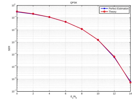
4.5 The SER curve for uncoded QPSK resulting from simulation matches the theoretical one. . . 44
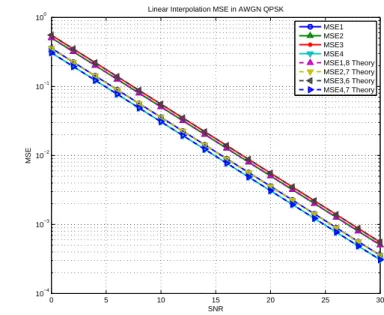
4.6 MSE performance for uncoded QPSK resulting with linear interpolation, an-tenna 0. . . 45
4.7 SER performance for uncoded QPSK resulting from linear interpolation. . . 45
4.8 MSE performance of Wiener filtering channel estimation for uncoded QPSK, antenna 0. Autocorrelation and cross-correlation are obtained by averaging over one subchannel. . . 50
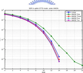
4.9 MSE performance of Wiener filtering channel estimation for uncoded QPSK, antenna 0. Autocorrelation and cross-correlation are obtained by averaging over ten subchannels. . . 51 4.10 Comparrision of SER performance with using Wiener filtering and linear
4.11 Comparrision of MSE performance with using Wiener filtering and linear in-terpolation channel estimation in STTD under QPSK modulation in AWGN. 52 4.12 MSE and SER performance for uncoded QPSK under Wiener filtering and
linear interpolation channel estimations at different velocities in single-path Rayleigh fading channel with ρenv = 0. (a) MSE. (b) SER. . . 54
4.13 MSE and SER performance for uncoded QPSK under Wiener filtering and linear interpolation channel estimation at different velocities in SUI-2 channel with channel correlation ρenv = 0. (a) MSE. (b) SER. . . 55
4.14 MSE and SER performance for uncoded QPSK under Wiener filtering and linear interpolation channel estimation at different velocities in SUI-3 channel with channel correlation ρenv = 0. (a) MSE. (b) SER. . . 56
4.15 Two different subchannel sets of MSE and SER performance for uncoded QPSK under Wiener filtering averaging over one subchannel at different ve-locities in SUI-2 channel with channel correlation ρenv = 0. (a) MSE. (b)
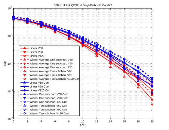
SER. . . 57 4.16 SER comparison between zero and nonzero antenna correlation (ρenv = 0.7)
in single-path Rayleigh fading. . . 58 4.17 SER comparison between zero and nonzero antenna correlation (ρenv = 0.5)
in SUI-2 channel. . . 59 4.18 SER comparison between zero and nonzero antenna correlation (ρenv = 0.4)
in SUI-3 channel. . . 60 5.1 Linear interpolation in STTD mode at antenna 0. . . 63 5.2 Wiener filtering in STTD mode at antenna 0. . . 64
5.3 Block diagram of the simulated system. . . 65
5.4 SER for uncoded QPSK resulting from simulation compared with theory. . . 66
5.5 MSE and SER performance for uncoded QPSK resulting from simulation with Wiener filtering and linear interpolation in AWGN channel. (a) MSE. (b) SER. . . 69
5.6 MSE and SER performance for uncoded QPSK resulting from simulation with Wiener filtering and linear interpolation at different velocities in single-path Rayleigh fading channel with ρenv = 0. (a) MSE. (b) SER. . . 70
5.7 MSE and SER performance for uncoded QPSK resulting from simulation with Wiener filtering and linear interpolation at different velocities in SUI-2 channel with ρenv = 0. (a) MSE. (b) SER. . . 71
5.8 MSE and SER performance for uncoded QPSK resulting from simulation with Wiener filtering and linear interpolation at different velocities in SUI-3 channel with ρenv = 0. (a) MSE. (b) SER. . . 72
5.9 SER comparison of zero and nonzero antenna correlations (ρenv = 0.7) in single-path Rayleigh fading. . . 73
5.10 SER comparison of zero and nonzero antenna correlations (ρenv = 0.5) in SUI-2. 74 5.11 SER comparison of zero and nonzero antenna correlations (ρenv = 0.4) in SUI-3. 74 6.1 The DSP on the Sundance board [21]. . . 76
6.2 Block diagram of the TMS320C6416 DSP [21]. . . 78
6.3 Pipeline phases of TMS320C6416 DSP [21]. . . 79
6.5 Code development flow for TI C6000 DSP [27]. . . 88 7.1 fix point simulation flow. . . 93 7.2 Uplink channel estimation performance under fixed- and floating-point
com-putation in AWGN. (a) MSE. (b) SER. . . 94 7.3 Uplink channel estimation performance under fixed- and floating-point
com-putation in single-path Rayleigh fading. (a) MSE. (b) SER. . . 95 7.4 Uplink channel estimation performance under fixed- and floating-point
com-putation in SUI-2 channel. (a) MSE. (b) SER. . . 96 7.5 Uplink channel estimation performance under fixed- and floating-point
com-putation in SUI-3 channel. (a) MSE. (b) SER. . . 97 7.6 Uplink channel estimation performance under fixed- and floating-point
com-putation in Vehicular A channel. (a) MSE. (b) SER. . . 98 7.7 MSE and SER under fixed- and floating-point computation in AWGN. (a)
MSE. (b) SER. . . 99 7.8 Downlink channel estimation performance under fixed- and floating-point
computation in single-path Rayleigh fading. (a) MSE. (b) SER. . . 100 7.9 Downlink channel estimation performance under fixed- and floating-point
computations in SUI-2 channel. (a) MSE. (b) SER. . . 101 7.10 Downlink channel estimation performance under fixed- and floating-point
computation in SUI-3 channel. (a) MSE. (b) SER. . . 102 7.11 Downlink channel estimation performance under fixed- and floating-point
computation in Vehicular A channel (a) MSE. (b) SER. . . 103 7.12 Wiener filtering C code block diagram. . . 105
7.13 FIXED.H. . . 106
7.14 linear interpolation. . . 107
7.15 Part of assembly code of function linear interpolaton. . . 108
List of Tables
2.1 OFDMA Uplink Subcarrier Allocations [6], [7] . . . 16
2.2 OFDMA Downlink Subcarrier Allocation Under PUSC [6], [7] . . . 23
4.1 αi of Eight Data Subcarriers at Antenna 0. . . 37
4.2 OFDMA Uplink Parameters . . . 40
4.3 Channel Profiles of SUI-2 and SUI-3 [17] . . . 41
4.4 Power-Delay Profile of the ETSI Vehicular A Channel . . . 42
4.5 Mean Delay and RMS Delay Spread . . . 42
4.6 MSE of Eight Data Subcarriers at Antennas 0 and 1 . . . 44
5.1 OFDMA Downlink Parameters . . . 62
6.1 Execution Stage Length Description for Each Instruction Type [21] . . . 80
6.2 Functional Units and Operations Performed (Part 1 of 2) [21] . . . 81
6.3 Functional Units and Operations Performed (Part 2 of 2) [21] . . . 82
7.1 OFDMA Uplink DSP Load Under 1024-FFT with 10 Subchannel . . . 105 7.2 OFDMA Downlink DSP Load Under 1024-FFT, Major Group 0 with STC . 106
Chapter 1
Introduction
Orthogonal frequency division multiple access (OFDMA) has emerged as one of the prime multiple access schemes for broadband wireless networks (e.g., IEEE 802.16 Mobile WiMAX, IEEE 802.20 and 3G LTE). As a special case of multicarrier multiple access schemes, OFDMA exclusively assigns each subchannel to only one user, eliminating intra-cell interference [1]. In frequency selective channels, an intrinsic advantage of OFDMA is its capability to exploit the so-called multiuser diversity provided by multipath channels. Other advantages of OFDMA include finer granularity and better link budget [1]. OFDMA can be easily generated using an inverse fast Fourier transform (IFFT) and received using a fast Fourier transform (FFT). The IEEE 802.16 standard committee has developed a group of standards for wireless metropolitan area networks (MANs). OFDMA is used in the 2 to 11 GHz systems. The IEEE Standard 802.16-2004 is for broadband wireless access systems that provide a variety of wireless access services to fixed outdoor and indoor users. The 802.16e is designed to support terminal mobility, and currently it can serve terminals with a speed up to 120 km/h [2].
Multiple-antenna techniques can be used to increase diversity and improve the bit error rate (BER) performance of wireless systems, increase the cell range, increase the transmitted
data rate through spatial multiplexing, and/or reduce interference from other users. The WiMAX Forum has selected two different multiple antenna profiles for use on the downlink and uplink. One of them is based on the space-time code (STC) proposed by Alamouti for transmit diversity [3], and the other is a 2x2 spatial multiplexing scheme.
This thesis focuses on the channel estimation methods for IEEE802.16e WirelessMAN-OFDMA multi-input multi-output (MIMO) systems. We construct the multipath channel simulator to simulate the MIMO system in IEEE 802.16e and study the performance of different channel estimation methods. And we consider software implementation of the channel estimation using a digital signal processor (DSP).
The thesis is organized as follows. First, in chapter 2, we introduce the OFDMA specifica-tions in IEEE 802.16e, especially its MIMO mode of operation. In chapter 3, various channel estimation techniques are introduced. In chpter 4, we discuss the performance of channel estimation in uplink transmission and in chpter 4, we show the performance of downlink channel estimation. It is seen that, due to modeling errors in parameter estimations, linear interpolation perfors better than Wiener filtering. In chapter 6, we describe the implemen-tation platform, which consists of a Texas Instruments’ TMS320C6416 DSP on a Sundance compancy’s Carrier board. In chapter 7, we present some DSP implementation issues and fixed-point simulation results. Finally, chapter 8 gives the conclusion and points out some potential future work.
Chapter 2
Introduction to IEEE802.16e OFDMA
and MIMO Systems
We first introduce the basic concepts of the OFDMA and MIMO techniques for multicarrier modulation. The specifications of IEEE 802.16e are introduced afterwards.
2.1
Overview of OFDMA [4], [5]
Orthogonal frequency-division multiple-access (OFDMA) is a major multiple access scheme considered for future wireless systems. In an OFDMA system, several users simultaneously transmit their data by modulating mutually exclusive sets of orthogonal subcarriers. Thus each user’s signal can be separated easily in the frequency domain. One typical structure is the subband OFDMA, which divides all available subcarriers into a number of subbands. Each user is allowed to use one or more available subbands for the data transmission. Pi-lot symbols are employed for the estimation of channel state information (CSI) within the subbands. Besides multiuser diversity, robustness to narrowband interference and capability of channel assignment are two other advantages of OFDMA. Figure 2.1 shows an OFDMA network in which active users simultaneously communicate with the base station (BS).
Figure 2.1: Discrete-time model of the baseband OFDMA system (from[4]).
2.1.1
Cyclic Prefix
Cyclic prefix (CP), or guard time, is used to overcome the intersymbol interference (ISI) and interchannel interference (ICI) problems. The multiuser channel is assumed to be sub-stantially invariant within one OFDMA symbol duration. The symbol timing mismatch is assumed to be smaller than the CP duration. In this scenario, users do not interfere each other in the frequency domain.
A CP is a copy of the last part of the OFDMA symbol (see Fig. 2.2). It is used to collect multipath propgation effects of the last symbol so as to maintaining the orthogonality of the tones. However, the transmitter energy increases with the length of the guard time while the receiver energy remains the same (since the cyclic extension is discarded in the receiver), so there is a 10log(1 − Tg/(Tb+ Tg))/log(10) dB loss in Eb/N0.
Figure 2.2: Time structure of OFDMA symbol (from [6]).
2.1.2
Discrete-Time Baseband Equivalent System Model
The material in this subsection is mainly taken from [5]. Consider an OFDMA system with
M active users sharing a bandwidth of B =1
T Hz (where T is the sampling period) as shown in
Fig. 2.3. The system consists of K subcarriers, of which Ku are useful subcarriers (excluding
guard bands and DC subcarrier). The users are allocated non-overlapping subcarriers in the spectrum depending on their needs.
The discrete time baseband channel consists of L multipath components and has the form h(l) = L−1 X m=0 hmδ(l − lm) (2.1)
where hm is a zero-mean complex Gaussian random variable with E[hih∗j] = 0 for i 6= j. In
frequency domain,
H = F h (2.2)
where H = [H0, H1, ..., HK−1]T, h = [h0, ..., hL−1, 0, ..., 0]T and F is K-point DFT matrix.
The impulse response length lL−1 is upper bounded by the length of CP (Lcp).
The received signal in frequency domain is given by
Yn=
M
X
i=1
Figure 2.3: Discrete-time baseband equivalent of an OFDMA system with M users (from [5]).
where Xi,n = diag(Xi,n,0, ..., Xi,n,K−1) is a K × K diagonal data matrix and Hi,n is the K × 1
channel vector (2.2) corresponding to the ith user in nth symbol. The noise vector Vn is distributed as CN (0, σ2I
K) where Ik is the K-dimensional identity matrix.
2.2
Introduction to MIMO System
In this section, we indroduce two MIMO transmission mechanisms that are used in WiMAX. One is called transmit diversity and the other spatial multiplexing. The material in this section is mainly taken from [8].
Figure 2.4: Schematic block diagram of Alamouti’s transmit diversity (from [8]).
2.2.1
Transmit Diversity
One MIMO transmission technique employed in WiMAX is the space-time coding (STC) scheme proposed by Alamouti [3] for transmit diversity. (In the IEEE 802.16e-2005 specifi-cations, this scheme is referred to as Matrix A.) This technique can be described as follows. Let (s1, s2) represent a group of two consecutive symbols in the input data stream to
be transmitted. During a first symbol period t1, transmit (Tx) antenna 1 transmits symbol
s1 and Tx antenna 2 transmits symbol s2. Next, during the second symbol period t2, Tx
antenna 1 transmits symbol s∗
2 and Tx antenna 2 transmits symbol −s∗1. Denote the channel
response (at the subcarrier frequency at hand) from Tx1 to the receiver (Rx) by h1 and the
channel response from Tx2 to the receiver by h2. The received signal samples corresponding
to the symbol periods t1 and t2 can be written as:
r1 = h1s1+ h2s2+ n1, (2.4)
r2 = h1s∗2+ h2s∗1+ n2, (2.5)
estimate the symbols s1 and s2: x1 = h∗1r1− h2r2∗ = ¡ |h1|2+ |h2|2 ¢ s1+ h∗1n1− h2n∗2, (2.6) x2 = h∗2r1+ h1r∗2 = ¡ |h1|2+ |h2|2 ¢ s2+ h∗2n1+ h1n∗2. (2.7)
These expressions clearly show that x1 (resp. x2) can be sent to a threshold detector to
estimate symbol s1 (resp. symbol s2) without interference from the other symbol. Moreover,
since the useful signal coefficient is the sum of the squared moduli of two independent fading channels, these estimations benefit from perfect second-order diversity, equivalent to that of Rx diversity under maximum-ratio combining (MRC). Alamouti’s transmit diversity can also be combined with MRC when two antennas are used at the receiver. In this scheme, the received signal samples corresponding to the symbol periods t1 and t2 can be written as
r11= h11s1+ h12s2+ n11, (2.8)
r12= h11s∗2 − h12s∗1+ n12, (2.9)
for the first receive antenna, and
r21= h21s1+ h22s2+ n21, (2.10)
r22= h21s∗2 − h22s∗1+ n22, (2.11)
for the second receive antenna. In these expressions, hjidesignates the channel response from
Tx i to Rx j, with i, j = 1, 2, and nij designates the noise on the corresponding channel. This
MIMO scheme does not give any spatial multiplexing gain, but it has 4th-order diversity, which can be fully recovered by a simple receiver as follows. The optimum receiver estimates
the transmitted symbols s1 and s2 using x1 = h∗11r11− h12r12∗ + h∗21r21− h22r22∗ = ¡|h11|2+ |h12|2+ |h21|2+ |h22|2 ¢ s1+ h∗11n11− h12n12∗ + h∗21n21− h22n∗22, (2.12) x2 = h∗12r11+ h11r12∗ + h∗22r21+ h21r∗22 = ¡|h11|2+ |h12|2+ |h21|2+ |h22|2 ¢ s2+ h∗12n11+ h11n12∗ + h∗22n21+ h21n∗22. (2.13)
These equations clearly show that the receiver fully recovers the fourth-order diversity of the 2 × 2 system.
2.2.2
Spatial Multiplexing
The second MIMO technique employed in WiMAX is the 2 × 2 spatial multiplexing (using the so-called matrix B = (s1, s2)T). This technique does not offer any diversity gain from
the Tx side. But it offers a diversity gain of 2 on the receiver side when detected using maximum-likelihood (ML) detection.
To describe the technique, we omit the time and frequency dimensions, leaving only the space dimension. The symbols transmitted by Tx1 and Tx2 in parallel are denoted s1 and
s2, respectively. Denoting by hji the channel response from Tx i to Rx j (i, j = 1, 2), the
signals received by the two Rx antennas are given by
r1 = h11s1+ h12s2+ n1, (2.14)
r2 = h21s1+ h22s2+ n2, (2.15)
which can be written in matrix form as · r1 r2 ¸ = · h11 h12 h21 h22 ¸ + · n1 n2 ¸ . (2.16)
symbols and decides in favor of (s1, s2) which minimizes the Euclidean distance
D(s1, s2) = |r1− h11s1− h12s2|2+ |r2− h21s1 − h22s2|2. (2.17)
2.3
Basic OFDMA Symbol Structure in IEEE 802.16e
The WirelessMAN-OFDMA PHY is based on OFDM modulation and is designed for nonline-of-sight (NLOS) operation in frequency bands below 11 GHz. For licensed bands, channel bandwidths allowed shall be limited to the regulatory provisioned bandwidth divided by any power of 2 no less than 1.0 MHz. The material in this section is mainly taken from [5] and [6].
2.3.1
OFDMA Basic Terms
We introduce some basic terms in OFDMA PHY. These definitions help us understand the concepts in subcarrier allocation and transmission of IEEE 802.16e OFDMA.
• Slot: A slot in OFDMA PHY is a two-dimensional entity spanning both a time and a
subchannel dimension. It is the minimum possible data allocation unit. For downlink (DL) PUSC (Partial Usage of SubChannels), one slot is one subchannel by two OFDMA symbols. For uplink (UL), one slot is one subchannel by three OFDMA symbols.
• Data region: In OFDMA, a data region is a two-dimensional allocation of a group of
contiguous subchannels in a group of contiguous OFDMA symbols. All the allocations refer to logical subchannels. A two-dimensional allocation may be visualized as a rectangle, such as the 4 × 3 rectangle shown in Fig. 2.5.
• Segment: A segment is a subdivision of the set of available OFDMA subchannels (that
may include all available subchannels). One segment is used for deploying a single instance of the MAC.
Figure 2.5: Example of the data region which defines the OFDMA allocation (from [6]).
Figure 2.6: OFDMA frequency description (from [6]).
2.3.2
Frequency Domain Description
An OFDMA symbol (see Fig. 2.6) is made up of subcarriers, the number of which determines the FFT size used. There are several subcarrier types:
• Data subcarriers: for data transmission.
• Pilot subcarriers: for various estimation purposes.
• Null subcarriers: no transmission at all, for guard bands and DC subcarrier.
2.3.3
Primitive Parameters
• BW : the nominal channel bandwidth.
• Nused: number of used subcarriers (which includes the DC subcarrier).
• n: sampling factor. This parameter, in conjunction with BW and Nused, determines
the subcarrier spacing and the useful symbol time. For channel bandwidths that are a multiple of 1.75 MHz, n = 8/7, else for channel bandwidths that are a multiple of any of 1.25, 1.5, 2 or 2.75 MHz, n = 28/25, else for channel bandwidths not otherwise specified, n = 8/7.
• G: the ratio of CP time to “useful” time, i.e., Tcp/Ts. The following values shall be
supported: 1/32, 1/16, 1/8, and 1/4.
2.3.4
Derived Parameters
The following parameters are defined in terms of the primitive parameters.
• NF F T: smallest power of two greater than Nused.
• Sampling frequency: Fs = f loor(n·BW/8000) × 8000.
• Subcarrier spacing: 4f = Fs/NF F T.
• Useful symbol time: Tb = 1/4f .
• CP time: Tg = G × Tb.
• OFDMA symbol time: Ts= Tb+ Tg.
Figure 2.7: Example of an OFDMA frame (with only mandatory zone) in TDD mode (from [7]).
2.3.5
Frame Structure
When implementing a time-division duplex (TDD) system, the frame structure is built from base station (BS) and subscriber station (SS) transmissions. Each frame in the DL trans-mission begins with a preamble followed by a DL transtrans-mission period and a UL transtrans-mission period. In each frame, the TTG and RTG shall be inserted between the downlink and uplink and at the end of each frame, respectively, to allow the BS to turn around. Fig. 2.7 shows an example of an OFDMA frame with only mandatory zone in TDD mode.
2.4
Uplink Transmission in IEEE 802.16e OFDMA
2.4.1
Data Mapping Rules
The UL mapping consists of two stages. In the first stage, the OFDMA slots allocated to each burst are selected. In the second stage, the allocated slots are mapped.
Stage 1: Allocate OFDMA slots to bursts. A UL allocation is created by selecting an integer number of contiguous slots according to the ordering of steps 1 to 3. This results in the general burst structure shown by the gray area in Fig. 2.8.
1) Segment the data into blocks sized to fit into one OFDMA slot.
2) Each slot shall span one or more subchannels in the subchannel axis and one or more OFDMA symbols in the time axis (see Fig. 2.8 for an example). Map the slots such that the lowest numbered slot occupies the lowest numbered subchannel in the lowest numbered OFDMA symbol.
3) Continue the mapping such that the OFDMA symbol index is increased. When the edge of the UL zone is reached, continue the mapping from the lowest numbered OFDMA symbol in the next available subchannel.
4)
Stage 2: Map OFDMA slots within the UL allocation.
1) Map the slots such that the lowest numbered slot occupies the lowest numbered sub-channel in the lowest numbered OFDMA symbol.
2) Continue the mapping such that the subchannel index is increased. When the last subchannel is reached, continue the mapping from the lowest numbered subchannel in the next OFDMA symbol that belongs to the UL allocation. The resulting order is shown by the arrows in Fig. 2.8.
Figure 2.8: Example of mapping OFDMA slots to subchannels and symbols in the uplink (from [7]).
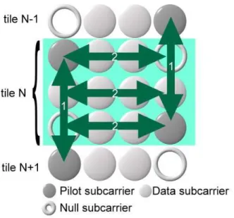
Figure 2.9: Structure of an uplink tile (from [6]).
Fig. 2.8 illustrates the order of OFDMA slots mapping to subchannels and OFDMA symbols.
2.4.2
Carrier Allocations
Consider the 1024-FFT PUSC permutation for example. Under it, the uplink supports 35 subchannels. Each transmission uses 48 data carriers as the minimal block of processing. Each new transmission for the uplink commences with the parameters as given in Table 2.1.
Table 2.1: OFDMA Uplink Subcarrier Allocations [6], [7]
Parameter Value Notes
Number of DC subcarriers
1 Index 512 (counting from 0)
Nused 841 Number of all subcarriers used within a symbol
Guard subcarriers: Left, Right
92,91
TilePermutation Used to allocate tiles to subchannels 11, 19, 12, 32, 33, 9, 30, 7, 4, 2, 13, 8, 17, 23, 27, 5, 15, 34, 22, 14, 21, 1, 0, 24, 3, 26, 29, 31, 20, 25, 16, 10, 6, 28, 18 Nsubchannels 35 Nsubcarriers 24 Ntiles 210 Number of subcarriers per tile
4 Number of all subcarriers within a tile Tiles per subchannel 6
A slot in the uplink is composed of three OFDMA symbols and one subchannel. Within each slot, there are 24 data subcarriers and 12 pilot subcarriers. The subchannel is con-structed from six uplink tiles, each having four successive active subcarriers with the config-uration as illustrated in Fig. 2.9.
The usable subcarriers in the allocated frequency band shall be divided into Ntilesphysical
tiles with parameters from Table 2.1. The allocation of physical tiles to logical tiles in subchannels is performed according to:
T iles(s, n) = Nsubchannels· n + (P t[(s + n) mod Nsubchannels] + UL P ermBase)mod Nsubchannels
where:
• T iles(s, n) is the physical tile index in the FFT with tiles being ordered consecutively
from the most negative to the most positive used subcarrier (0 is the starting tile index),
• n is the tile index 0..5 in a subchannel, • P t is the tile permutation,
• s is the subchannel number in the range 0..Nsubchannels− 1,
• UL P ermBase is an integer value in the range 0..69, which is assigned by a
manage-ment entity, and
• Nsubchannels is the number of subchannels for the FFT size given in Table 2.1.
After mapping the physical tiles to logical tiles for each subchannel, the data subcarriers per slot are enumerated by the following process:
1) After allocating the pilot carriers within each tile, indexing of the data subcarriers within each slot is performed starting from the first symbol at the lowest indexed subcarrier of the lowest indexed tile and continuing in an ascending manner through the subcarriers in the same symbol, then going to the next symbol at the lowest indexed data subcarrier, and so on. Data subcarriers shall be indexed from 0 to 47.
2) The mapping of data onto the subcarriers will follow the equation below. This equation calculates the subcarrier index (as assigned in item 1) to which the data constellation point is to be mapped:
Subcarrier(n, s) = (n + 13 · s) mod Nsubcarriers
where:
• Subcarrier(n, s) is the permutated subcarrier index corresponding to data
sub-carrier n is subchannel s,
Figure 2.10: PRBS generator for pilot modulation (from [6] and [7]).
• s is the subchannel number, and
• Nsubcarriers is the number of subcarriers per slot.
2.4.3
Pilot Modulation
The PRBS (pseudo-random binary sequence) generator depicted in Fig. 2.10 is used to produce a sequence, wk. The value of the pilot modulation, on subcarrier k, shall be derived
from wk.
For the mandatory tile structure in the uplink, pilot subcarriers shall be inserted into each data burst in order to constitute the symbol and they shall be modulated according to their subcarrier location within the OFDMA symbol. The pilot subcarriers shall be modulated according to <{ck} = 2 ¡1 2 − wk ¢ , ={ck} = 0. (2.18)
In all permutations except UL PUSC, downlink TUSC1, and the DL and UL STC permu-tations/modes, each pilot shall be transmitted with a boosting of 2.5 dB over the average non-boosted power of each data tone. That is, these pilot subcarriers shall be modulated
Figure 2.11: QPSK, 16-QAM, and 64-QAM constellations (from [6]). according to <{ck} = 8 3 ¡1 2 − wk ¢ · pk, ={ck} = 0. (2.19)
2.4.4
Data Modulation
The employed cosotellations are as shown in Fig. 2.11. The data bits are entered serially to the constellation mapper. Gray-mapped QPSK and Gray-mapped 16QAM shall be sup-ported, whereas the support of 64QAM (also Gray-mapped) is optional.
2.5
Downlink Transmission in IEEE 802.16e OFDMA
This section briefly introduces the specifications of IEEE 802.16e OFDMA PUSC downlink transmission. The material is mainly taken from [6] and [7].
2.5.1
Data Mapping Rules
The downlink data mapping rules are as follows:
1. Segment the data after the modulation block into blocks sized to fit into one OFDMA slot.
2. Each slot shall span one subchannel in the subchannel axis and one or more OFDMA symbols in the time axis, as per the slot definition mentioned before. Map the slots such that the lowest numbered slot occupies the lowest numbered subchannel in the lowest numbered OFDMA symbol.
3. Continue the mapping such that the OFDMA subchannel index is increased. When the edge of the Data Region is reached, continue the mapping from the lowest numbered OFDMA subchannel in the next available symbol.
Figure 2.12 illustrates the order of OFDMA slots mapping to subchannels and OFDMA symbols.
2.5.2
Preamble Structure and Modulation
Fig. 2.13 shows a downlink transmission period. The first symbol of the downlink trans-mission is the preamble. There are three types of preamble carrier-sets, which are defined bellow. The subcarriers in the preamable are modulated using a boosted BPSK modulation with a specific pseudo-noise (PN) code. The PN series modulating the pilots in the preamble can be found in [6, pp. 553–562].
The preamble carrier-sets are defined as
P reambleCarrierSetn= n + 3 · k, (2.20)
Figure 2.12: Example of mapping OFDMA slots to subchannels and symbols in the downlink in PUSC mode (from [7]).
Figure 2.13: Downlink transmission basic structure (from [6]).
• P reambleCarrierSetn specifies all subcarriers allocated to the specific preamble,
• n is the index of the preamble carrier-set indexed 0 ≤ 1 ≤ 2 and • k is a running index, 0 ≤ k ≤ 283.
Each segment uses one type of preamble out of the three sets in the following manner: For the preamble symbol, there are 172 guard band subcarriers on the left side and the right side of the spectrum. Segment i uses preamble carrier-set i, where i = 0, 1, 2. The DC subcarrier is not modulated at all and the appropriate PN is discarded. That is, the DC subcarrier is always zeroed.
The pilots in downlink preamble shall be modulated as
<{P reambleP ilotsModulated} = 4 ·√2 ·¡1 2 − wk ¢ , ={P reambleP ilotsModulated} = 0. (2.21)
2.5.3
Subcarrier Allocations
The OFDMA symbol structure is constructed using pilots, data and zero subcarriers. The symbol is first divided into basic clusters and zero carriers are allocated. The pilot tones are allocated first; what remains are data subcarriers, which are divided into subchannels that are used exclusively for data. Pilots and data carriers are allocated within each cluster.
Figure 2.14 shows the cluster structure with subcarriers from left to right in order of increasing subcarrier index. For the purpose of determining PUSC pilot location, even and odd symbols are counted from the beginning of the current zone. The first symbol in the zone is even. The preamble is not counted as part of the first zone. Table 2.2 summarizes the parameters of the OFDMA PUSC symbol structure.
The allocation of subcarriers to subchannels is performed using the following procedure: 1) Divide the subcarriers into a number (Nclusters) of physical clusters containing 14
Figure 2.14: Cluster structure (from [7]).
Table 2.2: OFDMA Downlink Subcarrier Allocation Under PUSC [6], [7]
Parameter Value Comments
Number of DC subcarriers
1 Index 512 (counting from 0) Number of guard subcarriers, left 92 Number of guard subcarriers, right 91 Number of used subcarriers (Nused)
841 Number of all subcarriers used within a symbol, including all possible allocated pilots and the DC carrier
Number of subcarriers per cluster
14 Number of clusters 60
Renumbering sequence Used to renumber clusters before allocation to subchannels: 6, 48, 37, 21, 31, 40, 42, 56, 32, 47, 30, 33, 54, 18, 10, 15, 50, 51, 58, 46, 23, 45, 16, 57, 39, 35, 7, 55, 25, 59, 53, 11, 22, 38, 28, 19, 17, 3, 27, 12, 29, 26, 5, 41, 49, 44, 9, 8, 1, 13, 36, 14, 43, 2, 20, 24, 52, 4, 34, 0 Number of data subcarriers in each symbol per subchannel
24 Number of subchannels 30 Basic permutation sequence 6 (for 6 subchannels) 12 3,2,0,4,5,1 Basic permutation sequence 4 (for 4 subchannels) 8 3,0,2,1
2) Renumber the physical clusters into logical clusters using the following formula: LogicalCluster =
RenumberingSequence(P hysicalCluster), first DL zone,
RenumberingSequence¡(P hysicalCluster+ 13 · DL P ermBase)mod Nclusters
¢
, otherwise.
3) Divids the clusters into six major groups. Group 0 includes clusters 0–11, group 1 clusters 12–19, group 2 clusters 20–31, group 3 clusters 32–39, group 4 clusters 40–51 and group 5 clusters 52–59. These groups may be allocated to segments. If a segment is being used, then at least one group shall be allocated to it. (By default group 0 is allocated to segment 0, group 2 to segment 1, and group 4 to segment 2.)
4) Allocate subcarriers to subchannel in each major group separately for each OFDMA symbol by first allocating the pilot subcarriers within each cluster and then taking all remaining data subcarriers within the symbol. The exact partitioning into subchannels is according to the equation below, called a permutation formula:
subcarrier(k, s) = Nsubchannels· nk+
©
ps[nk mod Nsubchannels]+
DL P ermBaseªmod Nsubchannels
where:
• subcarrier(k, s) is the subcarrier index of subcarrier k in subchannel s, • s is the index number of a subchannel, from the set [0..Nsubchannels − 1],
• nk = (k + 13 · s)mod Nsubcarriers , where k is the subcarrier-in-subchannel index
from the set [0..Nsubcarriers− 1],
• Nsubchannels is the number of subchannels (for PUSC use number of subchannels
• ps[j] is the series obtained by rotating basic permutation sequence cyclically to
the left s times,
• Nsubcarriers is the number of data subcarriers allocated to a subchannel in each
OFDMA symbol, and
• DL P ermBase is an integer from 0 to 31.
2.5.4
Pilot Modulation
Pilot subcarriers shall be inserted into each data burst in order to constitute the symbol. The PRBS (pseudo-random binary sequence) generator depicted in Fig. 2.10 shall be used to produce a sequence, wk.
Each pilot shall be transmitted with a boosting of 2.5 dB over the average non-boosted power of each data tone. That is, the pilot subcarriers shall be modulated according to
<{ck} = 8 3 ¡1 2− wk ¢ , ={ck} = 0. (2.22)
2.5.5
Data Modulation
Downlink transmission also employs the modulations shown in Fig. 2.11. gray-mapped QPSK and Gray-mapped 16QAM shall be supported, whereas the support of 64QAM (also Gray-mapped) is optional.
2.6
Space-Time Coding in IEEE 802.16e OFDMA
This section briefly introduces the space-time coding of IEEE 802.16e. The material is mainly taken from [6] and [7].
Figure 2.15: Illustration of STC (from [7]).
2.6.1
STC Using Two Antennas
STC (in some cases also termed STTD) or FHDC may be used on the DL to provide higher order (space) Tx diversity. Consider using two Tx antennas on the BS side and one reception antenna on the SS side. This scheme requires multiple-input single-output channel estimation. Decoding is very similar to maximum ratio combining.
Figure 2.15 shows Tx diversity insertion into the OFDMA chain. Each Tx antenna has its own OFDMA chain, but they have the same local oscillator for synchronization purposes. The two antennas transmit two different OFDMA data symbols in the same time. Time domain (space-time) or frequency domain (space-frequency) repetition is used.
2.6.2
STC/FHDC Configurations
Two transmission formats are allowed for the two-antenna configuration, each having its own capacity-diversity tradeoffs. The following matrices define the transmission formats with the row index indicating the antenna number and column index indicating the OFDMA symbol. The entries define the transmission from a subchannel used for this transmission configuration (the same operation is repeated for all subchannels used in this format). Transmission format
A uses matrix A (space time coding rate = 1): A = · S1 − (S2)∗ S2 (S1)∗ ¸ , (2.23)
whereas transmission format B uses matrix B (space time coding rate = 2):
B = · S1 S2 ¸ . (2.24)
2.6.3
Uplink Using STC
A user supporting transmission using STC configuration in the UL shall use a modified UL tile. The 2-Tx diversity data (STTD mode) or 2-Tx spatial multiplexing (SM mode) data can be mapped onto each subcarrier. The mandatory tile shall be modified to accommodate these configurations.
In STTD mode, the tiles shall be allocated to subchannels. The pilots in each tile shall be split between the two antennas, and the data subcarriers shall be encoded in pairs after constellation mapping, as depicted in Fig. 2.16. The data subcarriers transmitted from antenna 0 follow the original mapping.
2.6.4
STC Using Two Antennas in Downlink PUSC
In PUSC, the data allocation to cluster is changed to accommodate two antennas trans-mission with the same estimation capabilities, in which each cluster shall be transmitted twice from each antenna. Figure 2.14 is replaced by Figure 2.17 in the definition of PUSC permutation when STC is enabled. The pilot locations change in period of 4 symbols.
Symbols are counted from the beginning of the current zone. The first symbol in the zone is even. STC encoding is done on each pair of symbols 2n, 2n + 1 (n = 0, 1, ...).
Figure 2.16: Mapping of data subcarriers in STTD mode (from [7]).
Chapter 3
Channel Estimation Techniques
In this chapter, we discuss some channel estimation methods.
3.1
Pilot-Symbol-Aided Channel Estimation [9]
Channel estimators usually need some kind of pilot information as a point of reference. A fading channel requires constant tracking, so pilot information has to be transmitted more or less continuously. Decision-directed channel estimation can also be used. But even in this type of schemes, pilot information has to be transmitted regularly to mitigate error propagation.
3.1.1
The Least-Squares (LS) Estimator [10]
The simplest channel estimator one can imagine consists simply in dividing the received signal by the symbols that have been actually sent (and that are supposed to be known). Based on a priori known data, we can estimate the channel information on pilot carriers roughly by the least-squares (LS) estimator. An LS estimator minimizes the following squared error :
where Y is the received signal and X is a priori known pilots, both in the frequency domain and both being N × 1 vectors where N is the FFT size. ˆHLS is an N × N diagonal matrix
whose diagonal values are 0 except at pilot locations mi where i = 0, · · · , Np − 1:
ˆ HLS = Hm0,m0 · · · 0 · · · 0 · · · 0 0 · · · Hm1,m1 · · · 0 · · · 0 0 · · · 0 · · · Hm2,m2 · · · 0 0 · · · 0 · · · 0 · · · 0 0 · · · 0 · · · 0 · · · HmNp−1,HmNp−1 . (3.2)
Therefore, (3.1) can be rewritten as
[Y (m) − ˆHLS(m)X(m)]2, for all m = mi. (3.3)
Then the estimate of pilot subcarrier responses, based on only one observed OFDM symbol, is given by ˆ HLS(m) = Y (m) X(m) = X(m)H(m) + N(m) X(m) = H(m) + N(m) X(m) (3.4)
where N(m) is the complex white Gaussian noise on subcarrier m. We collect HLS(m) into
ˆ
Hp,LS, an Np× 1 vector where Np is the total number of pilots, as
ˆ Hp,LS = [Hp,LS(0) Hp,LS(1) · · · Hp,LS(Np− 1)]T = [Yp(0) Xp(0), Yp(1) Xp(1), . . . , Yp(Np−1) Xp(Np−1)] T. (3.5)
The LS estimate of Hp based on one OFDM symbol is susceptible to noise effects, and thus
an estimator better than the LS estimator is desirable.
3.1.2
The LMMSE Estimator [11]
The minimum mean-square error (MMSE) estimate has been shown to be better than the LS estimate for channel estimation in OFDM systems, but the major drawback of the MMSE estimate is its high complexity. A low-rank approximation results in a linear minimum mean squared error (LMMSE) estimator that uses the frequency-domain correlation of the channel
[11]. The linear minimum mean-square error channel estimator tries to minimize the mean squared error between the actual and the estimated channels, the latter obtained by a linear transformation applied to ˆHp,LS. The mathematical representation of the LMMSE estimator
on pilot signals is ˆ Hp,lmmse = RHpHp,LSR −1 Hp,LSHp,LSHˆp,LS = RHpHp(RHpHp+ σ 2 n(XpXHp )−1)−1Hˆp,LS (3.6)
where ˆHp,LS is the least-square estimate of Hp in (3.5), σn2 is the variance of the Gaussian
white noise, Xp is the vector of transmitted signal on pilot subcarriers, and the covariance
matrices are defined by
RHpHp,LS = E{HpH H p,LS}, (3.7) RHp,LSHp,LS = E{Hp,LSH H p,LS}, (3.8) RHpHp = E{HpH H p }. (3.9)
Note that there is a matrix inverse involved in the MMSE estimator, which must be calculated every time, and the computation of matrix inversion requires O(N3
p) arithmetic operations
[12].
3.2
Two-Dimensional Channel Estimators
By two-dimensional channel estimation, we mean that in addition to using channel informa-tion along the frequency domain, we also use channel informainforma-tion along the time domain to get better performance.
3.2.1
Linear Interpolation
After obtaining the channel response estimate at the pilot subcarriers, one may use interpola-tion to obtain the response at the rest of the subcarriers. Linear interpolainterpola-tion is a commonly
considered scheme due to its low complexity. It does the interpolation between two known data. That is, we use the channel information at two pilots obtained by the LS estimator to estimate the channel frequency response information at the data subcarriers between them. The channel estimates at data subcarrier k, mL < k < (m+1)L, using linear interpolation is given by [13]
He(k) = He(m + l) = (Hp(m + 1) − Hp(m))
l
L + Hp(m) (3.10)
where Hp(k), k = 0, 1, · · · , Np, are the channel frequency responses at pilot subcarriers, L is
the pilot subcarriers spacing, and 0 < l < L. In two-dimensional channel estimation, to suit the tile structure, we first interpolate in the time domain and then in the frequency domain.
3.2.2
2-D Wiener Filter [14]
The Wiener filter is the optimum (in the sense of minimum mean-squared error) linear filter or smoother or predictor, if the noise is additive.
Assume we have transmitted pilot signal vector p and received pilot signal vector ˆp containing noise. We want to find an estimate ˆh of the channel response h as a linear combination of ˆp. That means we want to find w that makes J (w) minimum, where w and
J (w) are defined as
ˆh = wTp, J(w) = Eˆ h|h − ˆh|2i. (3.11)
By applying the orthogonal projection theorem, we get
w = θTΦ−1 (3.12)
where θ is the cross-covariance vactor between p and h, and Φ is the auto-corvariance matrix between pilots.
Let k and l be the subcarrier number and the OFDM symbol number, respectively. The correlation values may be assumed as given by [15]
E£hk,lpˆ∗k0,l0
¤
= rf(k − k0)rt(l − l0) (3.13)
where rt(l)and rf(k) are the correlation functions in time and frequency, respectively. For
an exponentially decaying multipath power delay profile,
rf(k) =
1
1 + j2πτrmsk/T
(3.14) where 1/T is the subcarrier spacing, which is the inverse of the FFT interval T . For a time-fading signal with a maximum Doppler frequency fmax and a Clarke-Gans spectrum,
the time correlation function rt(l) is given by
rt(l) = J0(2πfmaxlTs) (3.15)
where J0 is the zeroth order Bessel function of the first kind and Ts is the OFDM symbol
Chapter 4
Simulation of STC Uplink Channel
Estimation
In this chapter we will simulate two different channel estimation methods for the in IEEE 802.16e OFDMA uplink system. One is linear interpolation and the other is Wiener filter. We evaluate the performance of both methods mainly by observing the mean square error (MSE) and the symbol error rate (SER).
4.1
Linear Interpolation
As described in chapter 2, the uplink transmission uses a tile structure to transmit pilot and data information. In the STC mode, one tile only contains two pilots. So we use tile (N −1) and tile (N +1) to interpolate the channel response of tile N, as shown in Fig. 4.1, to yield enough references for linear interpolation in frequency. Within three successive three tiles, we first estimate the channel response at each pilot position. Then we interpolate for the frequency response at each data subcarrier from the estimated pilot response in time domain. Lastly, we get the frequency response of the whole tile by interpolating the frequency response in the frequency domain.
Figure 4.1: Linear interpolation in STTD mode at antenna 0.
• Estimate the channel response at each pilot location by using the LS technique. • Use linear interpolation in the time dimension to get some data subcarrier responses
(makred 1 in Fig. 4.1).
• Estimate the channel responses of the remaining subcarriers in a tile by frequency
domain interpolation (marked 2 in Fig. 4.1).
4.2
Wiener Filtering
For two-dimensional Wiener filtering, we also choose three contiguous tiles to do channel estimation as depicted in Fig. 4.2. To do Wiener filtering, we have to know two parameters: autocorrelation of channel responses Φ at pilots and cross-correlation θ of channel response at data subcarriers and pilots. In the uplink, one subchannel contains six tiles. Thus we use the average over six tiles in the same subchannel to calculate Φ. That means if pilot subcarrier Pk’s channel response is pk and the estimate is ˆpk, where ˆpk = pk + nk with nk
Figure 4.2: Wiener filtering in STTD mode at Antenna 0.
being additive white Gaussian noise (AWGN), then we estimate Φ by
Φ = E ˆ p1pˆ∗1 pˆ1pˆ∗2 pˆ1pˆ∗3 pˆ1pˆ∗4 ˆ p2pˆ∗1 pˆ2pˆ∗2 pˆ2pˆ∗3 pˆ2pˆ∗4 ˆ p3pˆ∗1 pˆ3pˆ∗2 pˆ3pˆ∗3 pˆ3pˆ∗4 ˆ p4pˆ∗1 pˆ4pˆ∗2 pˆ4pˆ∗3 pˆ4pˆ∗4 ≈ 16 X one subchannel ˆ p1pˆ∗1 pˆ1pˆ∗2 pˆ1pˆ∗3 pˆ1pˆ∗4 ˆ p2pˆ∗1 pˆ2pˆ∗2 pˆ2pˆ∗3 pˆ2pˆ∗4 ˆ p3pˆ∗1 pˆ3pˆ∗2 pˆ3pˆ∗3 pˆ3pˆ∗4 ˆ p4pˆ∗1 pˆ4pˆ∗2 pˆ4pˆ∗3 pˆ4pˆ∗4 . (4.1)
To caculate θ, we first assume the channel response at data subcarrier hk is the 2-D linear
interpolation of four nearest pilot channel responses [16] as
hk= 3
X
i=0
αipi (4.2)
where αi are the linear interpolation weights. There are eight data subcarriers in a tile. We
list the αi of different data subcarrier in Table 4.1.
Table 4.1: αi of Eight Data Subcarriers at Antenna 0. Carrier α1 α2 α3 α4 1 2/3 2/9 0 1/9 2 1/3 4/9 0 2/9 3 2/3 0 1/3 0 4 4/9 1/9 2/9 2/9 5 2/9 2/9 1/9 4/9 6 0 1/3 0 2/3 7 2/9 0 4/9 1/3 8 1/9 0 2/9 2/3 E "Ã 3 X i=0 αipˆi ! ˆ p∗k # = E "Ã 3 X i=0 αipi+ 3 X i=0 αipini ! p∗k+ n∗k # = E "Ã 3 X i=0 αipi ! p∗ k # + αkσ02 (4.3)
where ni denotes the noise at pilot i and σ20 is the variance of the white Gaussian noise. Here
E [hjpˆ∗k] = E "Ã 3 X i=0 αipˆi ! ˆ p∗k # − αkσ02. (4.4)
As a result, the cross-correlation vector θk is given by
θk = E£ hkpˆ∗1 hkpˆ∗2 hkpˆ∗3 hkpˆ∗4 ¤ = E£ ¡P3i=0αipˆi ¢ ˆ p∗ 1 ¡P3 i=0αipˆi ¢ ˆ p∗ 2 ¡P3 i=0αipˆi ¢ ˆ p∗ 3 ¡P3 i=0αipˆi ¢ ˆ p∗ 4 ¤ −£ α0σ20 α1σ02 α2σ20 α3σ20 ¤ . (4.5)
Using the average over the six tiles of one subchannel to approximate the expectation oper-ation, we have θk ≈1 6 Ã X one subchannel £ ¡P3 i=0αipˆi ¢ ˆ p∗ 1 ¡P3 i=0αipˆi ¢ ˆ p∗ 2 ¡P3 i=0αipˆi ¢ ˆ p∗ 3 ¡P3 i=0αipˆi ¢ ˆ p∗ 4 ¤! −£ α0σ02 α1σ02 α2σ20 α3σ20 ¤ (4.6) where we can estimate σ2
0 by the power of the subcarriers in the guard band and those that
4.3
STC Decoding
After we have estimated the channel response, we can decode the STC, where the decoding method has been introduced before. If the channel responses are the same in neighboring subchannels as shown in Figure 4.3(a), then the received signals r1 and r2 are given by in,
absence of noise,
r1 = S1h0 − S2∗h1, r2 = S2h0+ S1∗h1. (4.7)
Then we can decode the received signal as
S1 = (r1h∗0+ r2∗h1) / ¡ |h0|2+ |h1|2 ¢ , S2 = (r2h∗0− r∗1h1) / ¡ |h0|2+ |h1|2 ¢ . (4.8)
But in a real channel, the neighboring channel responses may not be the same, especially when in high mobile speed, as shown in Figure 4.3(b),
r1 = S1h0 − S2∗h2, r2 = S2h1+ S1∗h3. (4.9)
So we decode by calculating
S1 = (r1h∗1+ r∗2h2) / (h0h∗1+ h2h∗3) ,
S1 = (r2h∗0− r∗1h3) / (h∗2h3+ h∗0h1) . (4.10)
4.4
Simulation Conditions
This section gives the system parameters and introduces the channel models used in our simulation work.
4.4.1
OFDMA Uplink System Parameters
In chapter 2, we introduced the primitive and the derived parameters of the system. The system parameters used in our simulation are listed in Table 4.2.
(a)
(b)
Figure 4.3: STTD transmission. (a) Neighboring channel responses are the same. (b) Responses are different.
4.4.2
Channel Models
We consider the following channel models: AWGN, single-path Rayleigh, SUI, and ETSI Vehicular A.
Erceg et al. [17] published a total of 6 different radio channel models for type G2 (i.e., LOS and NLOS) MMDS BWA systems in three terrain categories. The three types in suburban area are:
Table 4.2: OFDMA Uplink Parameters Parameters Values Bandwidth 10 MHz Carrier frequency 3.5 GHz NF F T 1024 Nused 841 Sampling factor n 28/25 G 1/8 Sampling frequency 11.2 MHz Subcarrier spacing 10.94 kHz Useful symbol time 91.43 µs
CP time 11.43 µs
OFDMA symbol time 102.86 µs Sampling time 89.29 ns
• C: flat terrain, light tree, and • B: between A and C.
The correspondence with the so-called SUI channels is as follows:
• C: SUI-1, SUI-2, • B: SUI-3, SUI-4, and • A: SUI-5, SUI-6.
In the above, SUI-1 and SUI-2 are Ricean multipath channels, whereas the other four are Rayleigh multipath channels [18]. The Rayleigh channels are more hostile and exhibit a greater RMS delay spread. And the SUI-2 represents a worst case link for terrain type C. We employ the SUI-2 and SUI-3 models in our simulation, but we use Rayleigh fading to model all the paths in these channels. The channel charateristics are as shown in Table 4.3. We also employ the ETSI Vehicular A model [19]. The model’s power delay profile is as shown in Table 4.4. The mean dealay and thd RMS delay are shiwn in Table 4.5.
Table 4.3: Channel Profiles of SUI-2 and SUI-3 [17]
4.5
Simulation Results
4.5.1
Simulation Flow
Figure 5.3 illustrates our simulated system. We assume perfect synchronization. After channel estimation, we calculate the MSE between the real channel and the estimated one,
Table 4.4: Power-Delay Profile of the ETSI Vehicular A Channel Tap Relative Delay (µs) Average Power (dB)
1 0 0 2 0.31 −1.0 3 0.71 −9.0 4 1.09 −10.0 5 1.73 −15.0 6 2.51 −20.0
Table 4.5: Mean Delay and RMS Delay Spread
Channel Mean Delay (µs) RMS Delay Spread(µs) SUI-2 0.0027 (0.0302 samples) 0.0428 (0.4793 samples) SUI-3 0.0413 (0.4626 samples) 0.1318 (1.4762 samples) Vehicular A 0.1325 (1.4840 samples) 0.1821 (2.0395 samples)
Figure 4.4: Block diagram of the simulated system.
where the average is taken over the subcarriers. The symbol error rate (SER) can also be obtained after demapping.
4.5.2
Validation of Simulation Model
Before considering multipath channels, we do simulation with an AWGN channel to validate the simulation model. We validate the model by comparing theoretical SER curves and the SER curves resulting from simulations, where we use C/C++ programing languange and
TI’s Code Composer Studio (CCS).
For an even number of bits per symbol, the SER of rectangular QAM is given by
Ps = 4 µ 1 − √1 M ¶ Q Ãr 3 M − 1 Es N0 ! (4.11) where
• M = number of symbols in modulation constellation; for example, M = 4 for QPSK,
M = 16 for 16QAM and M = 64 for 64QAM,
• Es = average symbol energy,
• N0 = noise power spectral density (W/Hz), and
• Q(x) = √1 2π R∞ x e−t 2/2 dt, x ≥ 0.
In Figure 4.5, the theoretical symbol error rate (SER) curve versus Es/N0 for uncoded QPSK
is plotted together with the SER curve resulting from simulation under no channel estimation error. This validates the simulation model.
4.5.3
Simulation Results and Analysis
For verification of the simulation results, note that the theoretical MSE for linear interpola-tion in AWGN is given by
MSE = E[|h − ˆh|2] = E[|h − 3 X i=0 αi(pi+ ni)|2] = E[| 3 X i=0 αini|2] = 3 X i=0 α2 iσ02. (4.12)
![Figure 2.3: Discrete-time baseband equivalent of an OFDMA system with M users (from [5]).](https://thumb-ap.123doks.com/thumbv2/9libinfo/7643009.138229/27.892.136.760.147.714/figure-discrete-time-baseband-equivalent-ofdma-m-users.webp)
![Figure 2.8: Example of mapping OFDMA slots to subchannels and symbols in the uplink (from [7]).](https://thumb-ap.123doks.com/thumbv2/9libinfo/7643009.138229/36.892.234.655.132.476/figure-example-mapping-ofdma-slots-subchannels-symbols-uplink.webp)
![Figure 2.12: Example of mapping OFDMA slots to subchannels and symbols in the downlink in PUSC mode (from [7]).](https://thumb-ap.123doks.com/thumbv2/9libinfo/7643009.138229/42.892.233.651.134.480/figure-example-mapping-ofdma-slots-subchannels-symbols-downlink.webp)

![Table 4.3: Channel Profiles of SUI-2 and SUI-3 [17]](https://thumb-ap.123doks.com/thumbv2/9libinfo/7643009.138229/62.892.129.758.156.859/table-channel-profiles-of-sui-and-sui.webp)