Simultaneous Application of Power Management Scheduling and Operation Delay Selection for Peak Power Minimization

全文

(1)Simultaneous Application of Power Management Scheduling and Operation Delay Selection for Peak Power Minimization Wei-Ting Yen, Chun-Hua Cheng, and Shih-Hsu Huang Department of Electronic Engineering, Chung Yuan Christian University, Chung Li, Taiwan, R.O.C. {g9376014, g9402601, shhuang}@cycu.edu.tw ABSTRACT Operation scheduling is the most important task in highlevel synthesis. Most conventional operation scheduling algorithms paid attention to the minimization of control steps or the minimization of resources. However, as the design complexity continues to increase, huge peak power may lead to logic errors due to voltage drops or reliability problems due to electromigration. As the popularization of portable and wireless communication, low power design is getting very important. An efficient power management method is to use control logic to shut down unused operations. On the other hand, longer operation delay, which implies smaller peak power, can be selected if no design constraint (timing and resource). In this paper, we present an ILP (integer linear programming) formulation to model the problem of simultaneous application of power management scheduling and operation delay selection for peak power minimization. Benchmark data consistently show that our approach minimizes the peak power within an acceptable run time.. 1: INTRODUCTIONS The peak power is the maximum power consumption of the integrated circuit at any instant during its execution. Huge peak power can cause many reliability problems, such as large voltage drop, large current density, and large heat dissipation. As the design complexity continues to increase, there is a demand to reduce the peak power at higher-level abstraction where the tradeoff is easier to understand. This paper, investigates the reduction of peak power during the stage of high-level synthesis. Therefore, several operation scheduling approaches [1,2] have been proposed to reduce the peak power. Note that Shiue [1] studied the peak power minimization under single supply voltage, while Mohanty, Ranganathan, and Chappidi [2] studied peak power minimization under multiple supply voltages. However, they [1,2] do not consider power management. Different from them, in this paper, we study the simultaneous application of power management scheduling and operation delay selection for peak power minimization. The basic idea of power. management is to shut down unused operations before their executions. On the other hand, longer operation delay, which implies smaller peak power, can be selected if no design constraint (timing and resource). An ILP (integer linear programming) formulation is proposed to model the simultaneous application of power management scheduling and operation delay selection for peak power minimization. Previous work [3,4] ever used the power management to reduce the average power. However, to the best of our knowledge, our paper is the first work that uses the simultaneous application of power management scheduling and operation delay selection to minimize the peak power.. 2: MOTIVATION We use the CDFG shown in Figure 1 to illustrate our motivation. The notation > denotes the control operation, the notation + denotes the addition operations, the notation - denotes the subtraction operations, and the notation * denotes the multiplication operation. Operations o1 and o4 are multiplexers. The control operation determines the output of the multiplexer. For example, if the result of operation o2 is true(T), the output of multiplexer o1 is the same as the output of operation o4; otherwise, the output of multiplexer o1 is the same as the output of operation o3.. - 248 -. Figure 1: A CDFG..

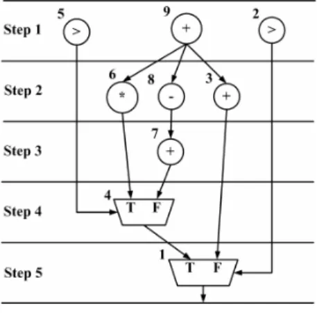
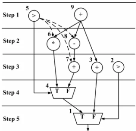
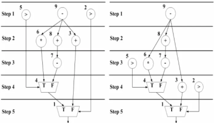
(2) Assume that the power consumptions of control operation, multiplexer, addition operation, subtraction operation, and multiplication operation are 4, 1, 3, 3, and 20, respectively. The power consumptions at control steps 1, 2, 3, 4, and 5 are 11, 26, 3, 1, and 1 respectively. The peak power is 26. However, in fact, due to the control operations, the outputs of some operations are not used under certain situations. For example, operation o6 and operation o7 are mutually exclusive. If the result of control operation o5 is 0, the output of operation o6 is not used; thus, we can add control logics to shut down operation o6 when the result of control operation o5 is 0. On the other hand, if the result of control operation o5 is 1, the output of operation o7 is not used. thus, we can add control logics to shut down operation o7 when the result of control operation o5 is 1. If the unused operations can be shut down, the power consumption can be reduced. However, due to dependency constraints and resource constraints, not all unused operations can be shut down. An unused operation can be shut down if and only if it is scheduled after the corresponding control operations. We use the CDFG shown in Figure 2 as an example. We use a dotted line, called soft edge, to denote the control logic that shuts down an operation when the unused condition occurs. The power consumptions at control steps 1, 2, 3, 4, and 5 are 7, 20, 6, 5, and 1, respectively. Therefore, the peak power is 20.. control steps 2, and 3 become 10, and 10, respectively. Therefore, the peak power is 10.. Figure 3: Simultaneous Application of Power Management Scheduling and Operation Delay Selection. Due to the deep-micron circuit design demand (e.g., reliability issue), we need to consider peak power in highlevel synthesis stage. Therefore, in this paper, we propose an ILP formulation to model the problem of simultaneous application of power management scheduling and operation delay selection... 3: ILP FORMULATION. Figure 2: Power Management scheduling Suppose that the power consumption of a multiplication operation is 20mW. If the multiplication operation is executed within one control step, the power consumption of each control step is 20 mW. On the other hand, if the multiplication operation is executed within two control steps, the power consumption of each control step is 10 mW. Using Figure 3 as an example, operation o6 can be delayed one clock cycle violating any design constraint (timing and resource). The power consumption of operation o6 at. In our ILP formulations, we use the notation xi,j,s to denote a binary variable (i.e., an 0-1 integer variable). Binary variable xi,j,s = 1, if and only if operation oi is scheduled into control step j and the slack of operation oi is exactly s clock cycles; otherwise, binary variable xi,j,s = 0. Clearly, we have 1 ≤ i ≤ n, 1 ≤ j ≤ t and 0 ≤ s ≤ t-1, where n is the number of operations in the data flow graph and t is the total number of control steps. Thus, intuitively, the total number of binary variables is n·t2. However, in fact, from the ASAP (as soon as possible) and ALAP (as late as possible) schedules, we can find that a lot of binary variables are redundant since their values are definitely 0. Therefore, we can prune these redundant binary variables without sacrificing the accuracy of the solution. The notations used in our ILP formulation are as below. (1) We use Ci to denote the set of control operations that can shut down operation oi when operation oi is unused. (2) The value |A| denotes the number of elements in the set A. (3) The value wi denotes the power consumption of operation oi. (4) We use the notation Yc,i to denote the control dependency from control operation oc to operation oi.. - 249 -.

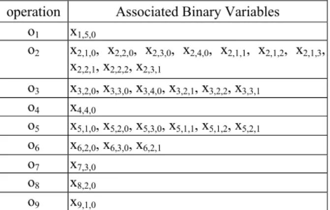
(3) (5). (6). (7). (8) (9) (10). (11). (12). (13). If the value Y c,i = 1, then there is a soft edge connects from control operation oc to operation oi. We use the notation Zc.i,j to denote the control dependency from control operation oc to operation oi and operation oi is scheduled into control step j. If the value Zc,i,j = 1, there is a soft edge from control operation oc to operation oi and operation oi is scheduled into control step j. We use the notation YA,i to denote the control dependency from control operations in the set A to operation oi. If the value YA,i = 1, there are soft edges that connects from control operations in the set A to operation oi. We use ZA,i,j to denote the control dependency from control operations in the set A to operation oi and operation oi is scheduled into control step j. If the value ZA,i,j = 1, there are soft edge that connects control operations in the set A to operation oi and operation oi is scheduled into control step j. The notation Hs denotes the set of unused operations under condition s. The delay of each operation oi is Di. The value Ei denotes the earliest possible control step of operation oi. Note that, we can use the ASAP calculation [5] to determine the value Ei for each operation oi. The value Li denotes the latest possible control step of operation oi. Note that, given the upper bound of number of control steps, we can use the ALAP calculation [5] to determine the value Li for each operation oi. We use FUk to denote the function unit k, and we say that oi ∈ FU k if and only if operation oi is assigned to be executed by the function unit FUk. The value Mk is the number of function unit k.. The minimal peak power problem can be formulated as the following ILP programming formulations. Minimize peak_power (Formula 1) Subject to For each operation oi Li − j. Li. ∑∑x j = Ei s = 0. i, j ,s. Li − j. ∑ ∑ ( j + D + s − 1) ⋅ x. i, j ,s. i. j = Ei s = 0. c ,i. ≤ YA,i. +. (Formula 6). A −1. For each operation ol and each operation YA , l ≤ Yi ,l. oi. ∈ A ⊆ Cl. (Formula 7). For each control step j, each operation oi, and each set A ⊆ Ci. YA,i + xi , j ,s ≤ Z A,i , j ,s + 1. (Formula 8). Z A ,i , j , s. (Formula 9). ≤ YA ,i. Z A,i , j , s ≤ xi , j , s. (Formula 10). For each control step j and each possible condition s n. Li − j. ∑ ∑. i =1 s = c − ( j + Di −1) n. ∑∑ ∑. wi ⋅ xi , j , s − s +1 Li − j. ∑. i =1 oi ∈H g A⊆ Ci s = c − ( j + Di −1). ( −1). A. ⋅. wi ⋅ Z A,i , j , s ≤ peak _ power s +1. (Formula 11) Formula 1 defines the objective function. Formula 2 states the constraint that every operation must be scheduled into a control step. Formula 3 ensures that the data dependency relationships are preserved. Formula 4 states the constraint that each function unit k at most executes under the number Mk in any control step. Formula 5, Formula 6, Formula 7, Formula 8, Formula 9, and Formula 10 describe the control dependency relationship due to adding soft edges. Formula 11 describe the peak power constraint for different conditions at each control step. We use the CDFG given in Figure 1 to illustrate our ILP formulation. Assume that the number of control steps is 4 and the delay of each operation is one control step. Figure 4 (a) and Fig. 4 (b) give the ASAP schedule and the ALAP schedule, respectively. According to the ASAP and ALAP schedules, we can prune all the redundant binary variables. Table 1 gives all the necessary (i.e., irredundant) binary variables associated with each operation. Table 2 gives all the binary variables associated with each possible control dependency. In the following, for each formula, we give an example to explain.. (Formula 2). =1. For each dependency relation oi→ol Li. ∑Y. oc ∈A. <. Lp − j. Lp. ∑ ∑ j⋅x. j = E p s =0. (Formula 3). p, j ,s. For each control step c and each island FUk Li − j. c. ∑ ∑ ∑. oi ∈FU k j = Ei s = c − ( j + Di −1). (Formula 4). xi , j , s ≤ M k. For each possible control dependency relation oi→ol L L −j L L −j (Formula 5) c. c. ∑ ∑(j+D. j = Ec s = 0. c. + s − 1) ⋅ xc , j , s <. i. i. ∑ ∑ j⋅x j = Ei s = 0. i, j,s. + (1 − Yc ,i ) ⋅ t. For each operation ol and the set A ⊆ Cl Figure 4 : (a) ASAP schedule. (b) ALAP schedule.. - 250 -.

(4) 2x6,2,0 + 3x6,2,1 + 3x6,3,0 < 4x4,4,0; 4x4,4,0 <5x1,5,0; 2x3,2,0 + 3x3,3,0 +4 x3,4,0 +3x3,2,1 + 4x3,2,2 + 4x3,3,1 < 5x1,5,0; 1x5,1,0 + 2x5,1,1+ 3x5,1,2 + 2x5,2,0 + 3x5,2,1 + 3x5,3,0 < 4x4,4,0; 1x 2,1,0 + 2x 2,2,0,+ 3x2,3,0,+ 4x2,4,0 + 2x2,1,1 + 3x2,1,2 + 4x 2,1,3 + 3x2,2,1 + 4x2,2,2 + 4x2,3,1 < 5x1,5,0;. operation Associated Binary Variables o1 x1,5,0 o2 x2,1,0, x2,2,0, x2,3,0, x2,4,0, x2,1,1, x2,1,2, x2,1,3, x2,2,1, x2,2,2, x2,3,1 o3 x3,2,0, x3,3,0, x3,4,0, x3,2,1, x3,2,2, x3,3,1 o4 x4,4,0 o5 x5,1,0, x5,2,0, x5,3,0, x5,1,1, x5,1,2, x5,2,1 o6 x6,2,0, x6,3,0, x6,2,1 o7 x7,3,0 o8 x8,2,0 o9 x9,1,0. Formula 4. Consider that there are three ALU operations o3, and o7 can be scheduled into control step 3. Suppose that we are given two ALUs and one multipliers. Then, we have x3,2,1+x3,2,2+x3,3,0+x3,3,1+x7,3,0 ≤ 2. All the constraints due to Formula 4 are listed in the following.. Table 1: Binary variables associated with each operation.. controller. Associated Binary Variables. Y{2},3, Y{2},6, Y{2},7, Y{2},8, Z{2},3,2,0, Z{2},3,2,1, Z{2},3,2,2, Z{2},3,3,0, Z{2},3,3,1, o2 Z{2},3,4,0, Z{2},6,2,0, Z{2},6,2,1, Z{2},6,3,0, Z{2},7,3,0, Z{2},8,2,0, Y{5},6, Y{5},7, Y{5},8, Z{5},6,2,0, Z{5},6,3,0, o5 Z{5},6,2,1, Z{5},7,3,0, Z{5},8,2,0, Y{2,5},6, Y{2,5},7, Y{2,5},8, Z{2,5},6,2,0, { o2, o5 } Z{2,5},6,2,1, Z{2,5},6,3,0, Z{2,5},7,3,0, Z{2,5},8,2,0, Table 2: Binary variables associated with soft edges.. Formula 5. If control operation o5 is schedule into control step 2, it is impossible to shut down operations o8. Thus, we have 1x5,1,0 + 2x5,1,1 + 3x5,1,2 + 2x5,2,0 + 3x5,2,1 + 3x5,3,0 < 2x8,2,0 + (1 - Y{5},8)*5. All the constraints due to Formula 5 are listed in the following.. Due to the page limit, we cannot list all the constraints of our ILP formulation for this CDFG. In the following, for each formula, we use an example to explain its meaning. Formula 2. Using operation o6 as an example, there is exactly one binary variable is true among all the 3 binary variables associated with operation o6. Thus, we have x6,2,0 + x6,2,1+ x6,3,0 = 1. All the constraints due to Formula 2 are listed in the following. x1,5,0 = 1; x 2,1,0 + x 2,2,0,+ x2,3,0,+ x2,4,0 + x2,1,1 + x2,1,2 + x 2,1,3 + x2,2,1 + x2,2,2 + x2,3,1 = 1; x3,2,0 + x3,3,0 + x3,4,0 + x3,2,1 + x3,2,2 + x3,3,1 = 1; x4,4,0 = 1; x5,1,0 + x5,1,1+ x5,1,2 + x5,2,0 + x5,2,1 + x5,3,0 = 1; x6,2,0 + x6,3,0 + x6,2,1 = 1; x7,3,0 = 1; x8,2,0 = 1; x9,1,0 = 1; Formula 3. Using the data dependency relation of o9→o6 as an example, operation o6 can be executed if and only if operation o9 has completed its execution. Thus, we have 2x9,1,0 < 2x6,2,0 + 2x6,2,1 + 3x6,3,0. All the constraints due to Formula 3 are listed in the following. x9,1,0 < 2x8,2,0; x9,1,0 < 2x3,2,0 + 3x3,3,0 +4 x3,4,0 +2x3,2,1 + 2x3,2,2 + 3x3,3,1; x9,1,0 < 2x6,2,0 + 2x6,2,1 + 3x6,3,0; 2x8,2,0 < 3x7,3,0; 3x7,3,0 < 4x4,4,0;. x3,2,1 + x3,2,2 + x3,3,0 + x3,3,1 + x7,3,0 ≤ 1; x3,2,1 + x3,2,2 + x3,2,0 + x8,2,0 ≤ 1; x3,2 + x7,2 + x9,2 ≤ 1; x9,1,0 ≤ 1; x6,2,0 ≤ 1; x6,3,0 ≤ 1; x6,2,1 ≤ 1;. 1x5,1,0 + 2x5,1,1 + 3x5,1,2 + 2x5,2,0 + 3x5,2,1 + 3x5,3,0 < 2x8,2,0 + (1 - Y{5},8)*5 1x5,1,0 + 2x5,1,1 + 3x5,1,2 + 2x5,2,0 + 3x5,2,1 + 3x5,3,0 < 3x7,3,0 + (1 - Y{5},7)*5 1x5,1,0 + 2x5,1,1 + 3x5,1,2 + 2x5,2,0 + 3x5,2,1 + 3x5,3,0 < 2x6,2,0 + 2x6,2,1 + 3x6,3,0 + (1 - Y{5},6)*5 1x2,1,0 + 2x2,2,0,+ 3x2,3,0,+ 4x2,4,0 + 2x2,1,1 + 3x2,1,2 + 4x 2,1,3 + 3x2,2,1 + 4x2,2,2 + 4x2,3,1 < 2x3,2,0 + 3x3,3,0 + 4x3,4,0 + 3x3,2,1 + 4x3,2,2 + 4x3,3,1 + (1 - Y{2},3)*5 1x2,1,0 + 2x2,2,0,+ 3x2,3,0,+ 4x2,4,0 + 2x2,1,1 + 3x2,1,2 + 4x 2,1,3 + 3x2,2,1 + 4x2,2,2 + 4x2,3,1 < 2x8,2,0 + (1 - Y{2},8)*5 1x2,1,0 + 2x2,2,0,+ 3x2,3,0,+ 4x2,4,0 + 2x2,1,1 + 3x2,1,2 + 4x 2,1,3 + 3x2,2,1 + 4x2,2,2 + 4x2,3,1 < 3x7,3,0 + (1 - Y{2},7)*5 1x2,1,0 + 2x2,2,0,+ 3x2,3,0,+ 4x2,4,0 + 2x2,1,1 + 3x2,1,2 + 4x 2,1,3 + 3x2,2,1 + 4x2,2,2 + 4x2,3,1 < 2x6,2,0 + 2x6,2,1 + 3x6,3,0 + (1 Y{2},6)*5 Formula 6, Formula 7, Formula 8, Formula 9, and Formula 10. Both control operation o2 and control operation o5 may shut down operation o7. Due to Formula 6, we have Y{2},7 + Y{5},7 ≤ Y{2,5},7 + 2 – 1. Due To Formula 7, we have Y{2,5},7 ≤ Y{2},7 and Y{2,5},7 ≤ Y{5},7. In other words, we have Y{2,5},7 = 1 if and only if both Y{2},7 =1 and Y{5},7 = 1. Due to Formula 8, we have Y{2,5},7 + x7,3,0 ≤ Z{2,5},7,3,0 + 1. Due to Formula 9, we have Z{2,5},7,3,0 ≤ Y{2,5},7. Due to Formula 10, we have Z{2,5},7,3,0 ≤ x7,3,0. In other words, we have Z{2,5},7,3,0 = 1 if and only if both Y{2,5},7 and x7,3,0 = 1. All the constraints due to Formula 6, Formula 7, Formula 8, Formula 9, and Formula 10 are listed in the following. Y{2},7 + Y{5},7 ≤ Y{2,5},7 +1; Y{2,5},7 ≤ Y{2},7;. - 251 -.

(5) Y{2,5},7 ≤ Y{5},7; Y{2},8 + Y{5},8 ≤ Y{2,5},8 +1; Y{2,5},8 ≤ Y{2},8; Y{2,5},8 ≤ Y{5},8; Y{2},6 + Y{5},6 ≤ Y{2,5},6 +1; Y{2,5},6 ≤ Y{2},6; Y{2,5},6 ≤ Y{5},6; Y{2,5},7 + x7,3,0 ≤ Z{2,5},7,3,0 + 1; Z{2,5},7,3,0 ≤ Y{2,5},7; Z{2,5},7,3,0 ≤ x7,3,0; Y{2,5},8 + x8,2,0 ≤ Z{2,5},8,2,0 + 1; Z{2,5},8,2,0 ≤ Y{2,5},8; Z{2,5},8,2,0 ≤ x8,2,0; Y{2,5},6 + x6,3,0 ≤ Z{2,5},6,3,0 + 1; Z{2,5},6,3,0 ≤ Y{2,5},6; Z{2,5},6,3,0 ≤ x6,3,0; Y{2,5},6 + x6,2,0 ≤ Z{2,5},6,2,0 + 1; Z{2,5},6,2,0 ≤ Y{2,5},6; Z{2,5},6,2,0 ≤ x6,2,0; Y{2,5},6 + x6,2,1 ≤ Z{2,5},6,2,1 + 1; Z{2,5},6,2,1 ≤ Y{2,5},6; Z{2,5},6,2,1 ≤ x6,2,1; Formula 11. Consider all the possible conditions at control step 2. If the output of control operation o2 is 0 and the output of control operation o5 is 0, we have 4x2,2,0 + 2x2,2,1 + 2x2,1,1 + 1.3x2,1,2 + 1x2,1,3 + 0.8x2,1,4 + 3x8,2,0 + 20x6,2,0 + 10x6,2,1 + 4x5,2,0 + 2x5,2,1 + 1.3x5,1,2 + 2x5,1,1 + 1.5x3,2,1 + 3x3,2,0 + 1x3,2,2 - 20Z{2},6,2,0 + 10Z{2,5},6,2,1 + 20Z{2,5},6,2,0 10Z{2},6,2,1 - 20Z{5},6,2,0 - 10Z{5},6,2,1 - 3Z{2},8,2,0 ≤ peak_power. If the output of control operation o2 is 0 and the output of control operation o5 is 1, we have 4x2,2,0 + 2x2,2,1 + 2x2,1,1 + 1.3x2,1,2 + 1x2,1,3 + 0.8x2,1,4 + 3x8,2,0 + 20x6,2,0 + 10x6,2,1 + 4x5,2,0 + 2x5,2,1 + 1.3x5,1,2 + 2x5,1,1 + 3x3,2,0 + 1x3,2,2 1.5x3,2,1 20Z{2},6,2,0 - 10Z{2},6,2,1 - 3Z{2},8,2,0 - 3Z{5},8,2,0 + 3Z{2,5},8,2,0 ≤ peak_power. If the output of control operation o2 is 1 and the output of control operation o5 is 0, we have 4x2,2,0 + 2x2,2,1 + 2x2,1,1 + 1.3x2,1,2 + 1x2,1,3 + 0.8x2,1,4 + 3x8,2,0 + 20x6,2,0 + 10x6,2,1 + 4x5,2,0 + 2x5,2,1 + 1.3x5,1,2 + 2x5,1,1 + 3x3,2,0 + 1.5x3,2,1 + 1x3,2,2 - 3Z{2},3,2,0 - 1.5Z{2},3,2,1 - 1Z{2},3,2,2 20Z{5},6,2,0 - 10Z{5},6,2,1 ≤ peak_power. If the output of control operation o2 is 1 and the output of control operation o5 is 1, we have 4x2,2,0 + 2x2,2,1 + 2x2,1,1 + 1.3x2,1,2 + 1x2,1,3 + 0.8x2,1,4 + 3x8,2,0 + 20x6,2,0 + 10x6,2,1 + 4x5,2,0 + 2x5,2,1 + 1.3x5,1,2 + 2x5,1,1 + 3x3,2,0 + 1.5x3,2,1 + 1x3,2,2 - 3Z{2},3,2,0 1.5Z{2},3,2,1 - 1Z{2},3,2,2 - 3Z{5},8,2,0 ≤ peak_power. All the constraints due to Formula 11 are listed in the following. Control step 1: 4x5,1,0 + 2x5,1,1 + 1.3x5,1,2 + 4x2,1,0 + 2x2,1,1 + 1.3x2,1,2 + 1x2,1,3 + 3x9,1,0 ≤ peak_power; Control step 2: o2 = 0 and o5 = 0 4x2,2,0 + 2x2,2,1 + 2x2,1,1 + 1.3x2,1,2 + 1x2,1,3 + 3x8,2,0 + 20x6,2,0 + 10x6,2,1 + 4x5,2,0 + 2x5,2,1 + 1.3x5,1,2 + 2x5,1,1 + 1.5x3,2,1 + 3x3,2,0 + 1x3,2,2 - 20Z{2},6,2,0 - 10Z{2},6,2,1 + 20Z{2,5},6,2,0 + 10Z{2,5},6,2,1 - 20Z{5},6,2,0 - 10Z{5},6,2,1 - 3Z{2},8,2,0 ≤ peak_power;. o2 = 0 and o5 = 1 4x2,2,0 + 2x2,2,1 + 2x2,1,1 + 1.3x2,1,2 + 1x2,1,3 + 3x8,2,0 + 20x6,2,0 + 10x6,2,1 + 4x5,2,0 + 2x5,2,1 + 1.3x5,1,2 + 2x5,1,1 + 3x3,2,0 + 1x3,2,2 +1.5x3,2,1 - 20Z{2},6,2,0 - 10Z{2},6,2,1 - 3Z{2},8,2,0 - 3Z{5},8,2,0 + 3Z{2,5},8,2,0 ≤ peak_power; o2 = 1 and o5 = 0 4x2,2,0 + 2x2,2,1 + 2x2,1,1 + 1.3x2,1,2 + 1x2,1,3 + 3x8,2,0 + 20x6,2,0 + 10x6,2,1 + 4x5,2,0 + 2x5,2,1 + 1.3x5,1,2 + 2x5,1,1 + 3x3,2,0 + 1.5x3,2,1 + 1x3,2,2 - 3Z{2},3,2,0 - 1.5Z{2},3,2,1 - 1Z{2},3,2,2 20Z{5},6,2,0 - 10Z{5},6,2,1 ≤ peak_power; o2 = 1 and o5 = 1 4x2,2,0 + 2x2,2,1 + 2x2,1,1 + 1.3x2,1,2 + 1x2,1,3 + 3x8,2,0 + 20x6,2,0 + 10x6,2,1 + 4x5,2,0 + 2x5,2,1 + 1.3x5,1,2 + 2x5,1,1 + 3x3,2,0 + 1.5x3,2,1 + 1x3,2,2 - 3Z{2},3,2,0 - 1.5Z{2},3,2,1 - 1Z{2},3,2,2 - 3Z{5},8,2,0 ≤ peak_power; Control step 3: o2 = 0 and o5 = 0 4x2,3,0 + 1.3x2,2,1 + 1x2,2,2 + 1x2,1,3 + 1.3x2,1,2 + 3x7,3,0 + 20x6,3,0 + 10x6,2,1 + 4x5,3,0 + 2x5,2,1 + 1.3x5,1,2 + 1.5x3,2,1 + 3x3,3,0 + 1x3,2,2 - 20Z{2},6,3,0 - 10Z{2},6,2,1 + 20Z{2,5},6,3,0 + 10Z{2,5},6,2,1 - 20Z{5},6,3,0 - 10Z{5},6,2,1 - 3Z{2},7,3,0 ≤ peak_power; o2 = 0 and o5 = 1 4x2,3,0 + 1.3x2,2,1 + 1x2,2,2 + 1x2,1,3 + 1.3x2,1,2 + 3x7,3,0 + 20x6,3,0 + 10x6,2,1 + 4x5,3,0 + 2x5,2,1 + 1.3x5,1,2 + 1.5x3,2,1 + 3x3,3,0 + 1x3,2,2 - 20Z{2},6,3,0 - 10Z{2},6,2,1 - 3Z{2},7,3,0 - 3Z{5},7,3,0 + 3Z{2,5},7,3,0 ≤ peak_power; o2 = 1 and o5 = 0 4x2,3,0 + 1.3x2,2,1 + 1x2,2,2 + 1x2,1,3 + 1.3x2,1,2 + 3x7,3,0 + 20x6,3,0 + 10x6,2,1 + 4x5,3,0 + 2x5,2,1 + 1.3x5,1,2 + 1.5x3,2,1 + 3x3,3,0 + 1x3,2,2 - 3Z{2},3,3,0 - 1.5Z{2},3,2,1 - 1Z{2},3,2,2 - 20Z{5},6,3,0 10Z{5},6,2,1 ≤ peak_power; o2 = 1 and o5 = 1 4x2,3,0 + 1.3x2,2,1 + 1x2,2,2 + 1x2,1,3 + 1.3x2,1,2 + 3x7,3,0 + 20x6,3,0 + 10x6,2,1 + 4x5,3,0 + 2x5,2,1 + 1.3x5,1,2 + 1.5x3,2,1 + 3x3,3,0 + 1x3,2,2 - 3Z{2},3,3,0 - 1.5Z{2},3,2,1 - 1Z{2},3,2,2 - 3Z{5},7,3,0 ≤ peak_power; Control step 4: o2 = 0 1x4,4,0 + 3x3,2,2 + 1.5x3,3,1 + 1x3,4,0 + 4x2,4,0 + 2x2,3,1 + 1.3x2,2,2 + 1x2,1,3 - 1Z{2},4,4,0 ≤ peak_power; o2 = 1 1x4,4,0 + 3x3,2,2 + 1.5x3,3,1 + 1x3,4,0 + 4x2,4,0 + 2x2,3,1 + 1.3x2,2,2 + 1x2,1,3 - 3Z{2},3,4,0 – 1.5Z{2},3,3,1 - 1Z{2},3,2,2 ≤ peak_power; Control step 5: 1x1,5,0 ≤ peak_power; After solving the ILP formulation, we have that x1,4,0 = x2,4,0 = x3,4,0 = x4,4,0 = x5,1,0 = x6,2,1 = x7,3,0 = x8,2,0 = x9,1,0 = Y5,6 = Y5,7 = Y5,8 = Z{5},6,2,1 = Z{5},7,3,0 = Z{5},8,2,0 = 1, and the values of other binary variables are 0.. 4: EXPERIMENTAL RESULTS The ILP solver is the Extended LINGO Release 8.0 running on a personal computer with P4-3.3GHz CPU and 1024M Bytes RAM. Seven benchmark circuits are used to test the effectiveness of our approach. Benchmark circuits. - 252 -.

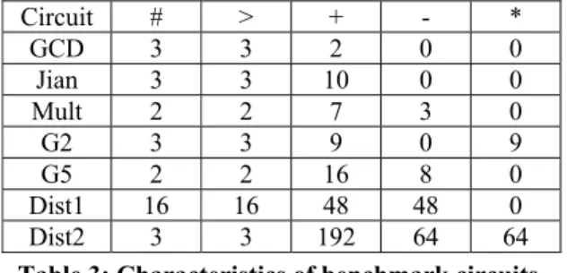
(6) GCD [6], Jian [7], Mult [8], G2 [9], G5 [10] are popular DSP applications and widely used in the high-level synthesis community, while benchmark circuits Dist1 and Dist2 are the representative functions adopted from the MediaBench suite [11]. In our experiments, the CPU time of each benchmark circuit is only few minutes. Table 3 gives the characteristics of benchmark circuits. The column # denotes the number of multiplexers. The column > denotes the number of comparison operations. The column + denotes the number of addition operations. The column - denotes the number of subtraction operations. The column * denotes the number of multiplication operations. Circuit # > + * GCD 3 3 2 0 0 Jian 3 3 10 0 0 Mult 2 2 7 3 0 G2 3 3 9 0 9 G5 2 2 16 8 0 Dist1 16 16 48 48 0 Dist2 3 3 192 64 64 Table 3: Characteristics of benchmark circuits.. GCD Jian Mult G2 G5 Dist1 Dist2. Constraints Peak Power Resources Steps [1] Ours Imp% 2 ALUs 5 6 5 17% 6 10 8 20% 3 ALUs 7 9 7 22% 3 ALUs 6 9 7 22% 2 MULs 8 46 38 17% 2 ALUs 9 43 22 49% 8 12 9 25% 4 ALUs 9 10 7 30% 38 13 10 23% 3 ALUs 39 10 8 20% 5 ALUs 99 22 18 18% 2 MULs 100 20 15 20% Table 4: Experimental results.. In this paper, we present an ILP formulation to model the peak power minimization problem via the combination of power management scheduling and operation delay selection. Benchmark data consistently show that our approach has significant peak power reduction. Compared with the peak power reduction via only operation scheduling, our average improvement achieves 27.2%.. ACKNOWLEDGMENTS This work was supported in part by the National Science Council of R.O.C. under the grant number NSC 93-2220-E-033-001.. REFERENCES. Table 4 gives our experimental results. For the purpose of comparisons, we also implement the power management scheduling approach proposed in [1]. The column Resources denotes the resource constraints. The column Steps denotes the number of control steps. The column [1] denotes the minimum peak power obtained by the approach of [1] (i.e., the minimum peak power achieved by operation scheduling). The column Ours denotes the minimum peak power obtained by our approach (i.e., the minimum peak power achieved by the simultaneous application of operation scheduling and power management). The column Imp% denotes the percentage of improvement. Circuit. 5: CONCLUSIONS. [1] W.T. Shiue, “High Level Synthesis for Peak Power Minimization using ILP”, Proc. of IEEE International Conference on Application-Specific Systems, Architectures, and Processors, pp. 103—112, 2000. [2] S.P. Mohanty, N. Ranganathan, and S.K. Chappidi, “Peak Power Minimization through Datapath Scheduling”, Proc. of IEEE Computer Society Annual Symposium on VLSI, pp. 121—126, 2003. [3] J. Monterio, S. Devadas, P. Ashar, and A. Mauskar, “Scheduling Technique to Enable Power Management”, Proc. of IEEE/ACM Design Automation Conference, pp. 349—352, 1996. [4] C. Chen and M. Sarrafzadeh, “Power Management Scheduling Technique for Control Dominated High Level Synthesis”, Proc. of IEEE Design, Automation and Test in Europe Conference and Exhibition, pp. 1016—1020, 2002. [5] C.T. Hwang, J.H. Lee, and Y.C. Hsu, “A Formal Approach to the Scheduling Problem in High Level Synthesis”, IEEE Trans. on Computer Aided Design of Integrated Circuits and Systems, vol. 10, no. 4, pp. 464—475, 1991. [6] F.F. Hsu, E.M. Rudnick, and J.H Patel, “Testability Insertion in Behavioral Descriptions”, Proc. of IEEE International Symposium on System Synthesis, pp. 139—144, 1996. [7] J. Li, R.K. Gupta “An Algorithm to Determine Mutually Exclusive Operations in Behavioral Descriptions”, Proc. of IEEE/ACM Design Automation and Test in Europe, pp. 457—465, 1998. [8] K. Wakabayashi and H. Tanaka, “Global Scheduling Independent of Control Dependencies Based on Condition Vectors”, Proc. of IEEE/ACM Design Automation Conference, pp. 112—115, 1992. [9] J. Siddhiwala and L.F. Chao, “Scheduling conditional dataflow graphs with resource sharing”, Proc. of IEEE International Symposium on VLSI, pp. 94—97, 1995. [10] T. Kim, J.W. Lin, and C.L. Lin, “A Scheduling Algorithm for Conditional Resource Sharing”, Proc. of IEEE/ACM International Conference on Computer Aided Design, pp. 84—87, 1991. [11] C. Lee, M. Potkonjak, and W.H. Maggione-Smith, “MediaBench: A Tool for Evaluating and Synthesizing Multimedia and Communications Systems,” Proc. of IEEE International Symposium on Microarchitecture, pp. 330—335, 1997.. - 253 -.

(7)