一個基於傳輸率與節能的異質無線感測網路群首推選策略研究

國

立

交

通

大

學

資訊科學與工程研究所

碩

士

論

文

一個基於傳輸率與節能的異質無線感測網路群首推

選策略研究

An election strategy of cluster head based on the transmission rate

and energy efficiency for Heterogeneous Wireless Sensor

Networks

研 究 生：謝培仁

指導教授：陳耀宗 教授

一個基於傳輸率與節能的異質無線感測網路群首推選策略研究

An election strategy of cluster head based on the transmission rate and

energy efficiency for Heterogeneous Wireless Sensor Networks

研 究 生：謝培仁 Student：Pei-Jen Hsieh

指導教授：陳耀宗 Advisor：Yaw-Chung Chen

國 立 交 通 大 學

資 訊 科 學 與 工 程 研 究 所

碩 士 論 文

Submitted to Institute of Computer Science and Engineering College of Computer Science

National Chiao Tung University in partial Fulfillment of the Requirements

for the Degree of Master

In

Computer Science

September 2014

Hsinchu, Taiwan, Republic of China

i

一個基於傳輸率與節能的異質無線感測網路群首推選策略研究

學生：謝培仁

指導教授：陳耀宗 博士

國立交通大學資訊科學與工程研究所

摘要

ii

An election strategy of cluster head based on the transmission rate and

energy efficiency for Heterogeneous Wireless Sensor Networks

Student：Pei-Jen Hsieh

Advisor：Dr. Yaw-Chung Chen

Institute of Computer Science and Engineering

National Chiao Tung University

Abstract

Heterogeneous wireless sensor network contains lots of nodes with different capabilities and energy. While comparing the traditional homogeneous wireless sensor network, utilizing the heterogeneity for the network can raise the throughput. In this thesis, we propose a scheme to balance energy load on each node, control the number of cluster head to save energy, and elect the node with higher bandwidth to be a cluster head to increase the throughput. Our scheme may be applied to the emerging machine to machine communications which usually consists of a large number of heterogeneous sensor nodes. Finally, we evaluate the performance of our proposed scheme by simulation and compare it with LEACH. The result shows that lifetime, energy consumption, and throughput perform much better than LEACH.

iii

Contents

1.2 Organization of the Thesis ... 4

Chapter 2 Background ... 5

2.1 Energy Model ... 5

2.2 Analysis of Routing Protocol ... 6

2.2.1 Direct Communication... 6

2.2.2 MTE multi-hop routing... 7

2.2.3 Clustering ... 8 2.3 Related Work ... 9 2.3.1 LEACH ... 9 2.3.2 LEACH-C ... 10 2.3.3 SEP ... 11 2.3.4 EDCS ... 12 2.3.5 EEPCA ... 13

Chapter 3 Proposed Scheme ... 14

3.1 Network Model ... 15

iv

3.2.1 Cluster Head Election Phase ... 17

3.2.2 Advertisement Phase ... 24

3.2.3 Cluster Set-Up Phase ... 25

3.2.4 Schedule Creation Phase ... 25

3.2.5 Data Transmission ... 25

3.2.6 Re-Clustering ... 26

3.2.7 Overview of ESCH ... 27

Chapter 4 Simulation and Results ... 28

4.1 Simulation Environment ... 28

4.2 Metrics of Performance ... 29

4.3 Simulation Results Analysis ... 31

4.3.1 Lifetime ... 31

4.3.2 Energy Consumption ... 33

4.3.3 Number of Packet Received ... 35

4.3.4 Number of Cluster Head ... 37

Chapter 5 Conclusions and Future Works ... 39

v

Table List

Table 4.1 The initial parameters for simulation. ... 28 Table 4.2 The setting of nodes for each type ... 29 Table 4.3 The time comparison for FND, HND and LND. ... 31

vi

Figure List

Figure 1.1 The architecture of WSN ... 1

Figure 2.1 First Order Radio Model ... 5

Figure 2.2 Direct Communication ... 7

Figure 2.3 MTE multi-hop routing ... 8

Figure 2.4 Clustering for WSN ... 8

Figure 3.1 Architecture of WSN and its components. ... 15

Figure 3.2 Organization of a round ... 16

Figure 3.3 The data structure of the table and its entry in Node i ... 18

Figure 3.4 Utilization level of each entry and the average utilization level. ... 19

Figure 3.5 Threshold examination. ... 21

Figure 3.6 Ranking by bandwidth and cluster head election. ... 23

Figure 3.7 Data Transmission time line ... 26

Figure 3.8 overview of ESCH ... 27

Figure 4.1 Number of alive nodes over time. ... 33

Figure 4.2 Total energy consumption over time ... 35

Figure 4.3 Number of packets received at BS over time. ... 36

Figure 4.4 Energy versus Number of Received Packets at BS ... 37

1

Chapter 1 Introduction

Due to the advances in Micro-Electro-Mechanical Systems technology, Wireless Sensor Networks (WSNs) [1] [2] have gained worldwide attention in recent years. WSNs have great potential for many applications such as military, natural disaster, biomedical health, and seismic sensing. In military, a WSN can assist in intrusion detection and identification. With natural disaster, sensor nodes can sense and detect the environment to forecast disasters before occurring. For seismic sensing, sensors can detect the earthquakes and eruptions.

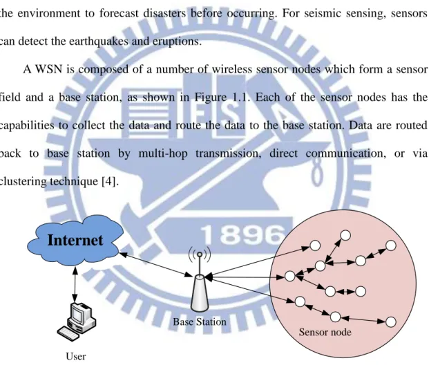
A WSN is composed of a number of wireless sensor nodes which form a sensor field and a base station, as shown in Figure 1.1. Each of the sensor nodes has the capabilities to collect the data and route the data to the base station. Data are routed back to base station by multi-hop transmission, direct communication, or via clustering technique [4].

Base Station

Internet

Sensor node User

Figure 1.1 The architecture of WSN

The positions of sensor nodes don’t need to be predetermined. This allows random deployment when the environment is inaccessible by humans. On the other hand, it also means that sensor network protocols and algorithms should have the capability of self-organizing. Instead of transmitting raw data to the nodes that is

2

responsible to fuse, sensor nodes use their processing abilities to filter the raw data which they sensed from the environment.

Unlike traditional networks, a WSN has its own constraints in each sensor node, such as limited amount of energy, short communication range, limited computational capability and memory. One of the most important constraints is limited amount of energy which is generally irreplaceable. The energy available at each sensor for sensing and communication is limited and globally affects the application time.

Wireless Sensor Network can be classified into two types according to the difference between sensor nodes [5]. In homogeneous sensor networks, all the sensor nodes are identical in terms of energy, hardware capability. While in a heterogeneous WSN, sensor nodes can be divided into two or more type according to initial energy and hardware capability. In heterogeneous WSN, there are three common types of resource heterogeneity: computational heterogeneity, link heterogeneity, and energy heterogeneity [6].

 Computational heterogeneity: A heterogeneous node has a more powerful processor and more memory than a normal node.

 Link heterogeneity: A heterogeneous node has higher bandwidth and more powerful transceiver than a normal node.

 Energy heterogeneity: A fraction of heterogeneous sensor nodes have different energy initially.

1.1 Motivation

Placing some heterogeneous nodes into WSN, it is an effective way to increase network lifetime and reliability. While the sensor nodes with better computational and link capabilities, the packets received from sensors can be processed and transmitted

3 faster than homogeneous WSN.

Previous researches about clustering for WSN have been proposed, such as LEACH [7], and LEACH-C [8] that are proposed under homogeneous WSN. However, the cluster-head selection strategies of LEACH and LEACH-C are not appropriate for heterogeneous WSN. In LEACH, it doesn’t consider the residual energy to avoid one node draining its energy quickly and to control the number of cluster head in each round. Moreover, these researches are studied under homogeneous sensor nodes, and the resource heterogeneities are not considered. The researches about heterogeneous WSN are proposed such as SEP [12], EDCS [13], and EACP [14].

4

1.2 Organization of the Thesis

The rest of the thesis is organized as followings. Chapter 2 shows the background and related work of our proposed scheme. Then Chapter 3 presents the proposed design in detail. Next, Chapter 4 discuss and analyzes the simulation result. Finally, in Chapter 5, the conclusion and future work will be described.

5

Chapter 2 Background

There three sections in this chapter. The first section is the energy model that we use in our scheme. In the second section, we will discuss the typical routing protocol of WSN and focus on the analysis of energy. Finally, we will present the related work and the relative discussion.

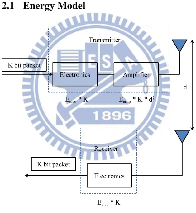
2.1 Energy Model

Figure 2.1 First Order Radio Model

Energy dissipation models are very important in WSNs, as they can be utilized to compare the performance of different communication protocols from the energy point

6

of view. A very simple and commonly used energy dissipation model is the First Order Model which is introduced in [9]. The model, shown in Fig 2.1, considers that to transmit a K-bit packet from sender to receiver over a distance d, the system spends: ETx (K, d) = Eelec-Tx (K) + Eamp-Tx (K, d) (2.1) ETx (K, d) = { 𝐸𝑒𝑙𝑒𝑐× 𝐾 + 𝐾 × 𝜖𝑓𝑠× 𝑑2, 𝑑 < 𝑑0 𝐸_{𝑒𝑙𝑒𝑐}× 𝐾 + 𝐾 × 𝜖_𝑓𝑠× 𝑑4_{, 𝑑 ≥ 𝑑} 0 (2.2)

Where ETx (K, d) is the energy consumed by the transmitter to send a K-bit long

packet over distance d, Eelec-Tx (K) is the energy used by the electronics of the

transmitter, and Eamp-Tx (K, d) is the energy expended by the amplifier. Similarly, at the

receiving node, to receive the message the transceiver spends:

ERx (K) = Eelec-Rx (K) (2.3)

ERx (K) = 𝐸𝑒𝑙𝑒𝑐× 𝐾 (2.4)

Where ERx (K) is the energy consumed by the receiver in receiving a K-bit long

packet, which is given by the energy used by the electronics of the receiver Eelec-Rx(K).

2.2 Analysis of Routing Protocol

There have been several network routing protocols proposed for wireless networks that can be examined in the context of wireless sensor networks. We present three such protocols, namely direct communication with the base station, minimum-transmission-energy (MTE) multi-hop routing, and clustering technique in the following sections.

2.2.1

Direct Communication

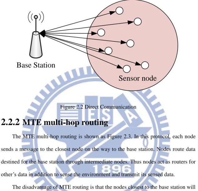
As shown in Figure 2.2, using a direct communication protocol, each sensor node sends its data directly to the base station. If the base station is far away from the nodes, direct communication will require a large amount of transmit power since d in Equation 2.1 is large. This will quickly drain the battery of the nodes and reduce the

7 overall system lifetime.

Base Station

Sensor node

Figure 2.2 Direct Communication

2.2.2

MTE multi-hop routing

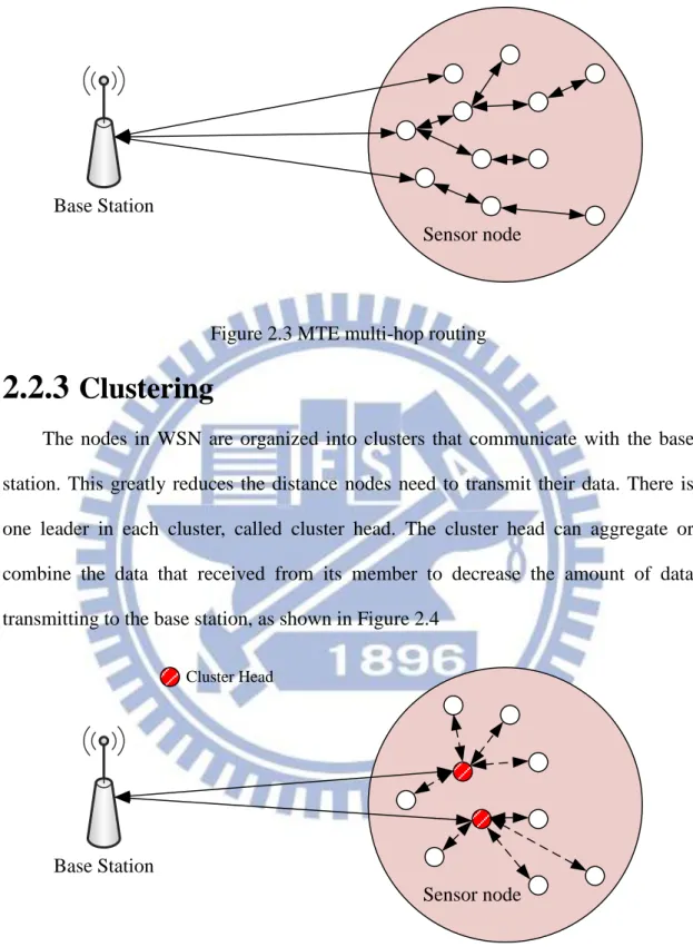
The MTE multi-hop routing is shown as Figure 2.3. In this protocol, each node sends a message to the closest node on the way to the base station. Nodes route data destined for the base station through intermediate nodes. Thus nodes act as routers for other’s data in addition to sense the environment and transmit its sensed data.

The disadvantage of MTE routing is that the nodes closest to the base station will be used to route a lot of messages to the base station. Thus these nodes will die out quickly, causing the energy that is required to transmit to the base station increase and more nodes will die faster.

8 Base Station

Sensor node

Figure 2.3 MTE multi-hop routing

2.2.3

Clustering

The nodes in WSN are organized into clusters that communicate with the base station. This greatly reduces the distance nodes need to transmit their data. There is one leader in each cluster, called cluster head. The cluster head can aggregate or combine the data that received from its member to decrease the amount of data transmitting to the base station, as shown in Figure 2.4

Base Station

Sensor node

Cluster Head

9

2.3 Related Work

2.3.1 LEACH

LEACH is a self-organizing, adaptive clustering protocol that uses randomization to distribute the energy load among the sensor in the WSN. The nodes organize themselves into clusters, with one cluster head to manage the cluster. The operation of LEACH is broken up into rounds. Each round begins with set-up phase for clustering the nodes and the following steady-state phase for data transferring to the base station.

During set-up phase of LEACH, each node decides whether or not to become a cluster-head node for this current round. The decision of cluster head is based on the percentage of cluster heads for the network and the number of times the node has been a cluster head so far. The node chooses a random number between 0 and 1. If the number is less than the threshold T(n), the node becomes a cluster head for the current round. The threshold is set in Equation:

𝑇(𝑛) = {

𝑃

1−𝑃×(𝑟 𝑚𝑜𝑑1_𝑝) 𝑖𝑓 𝑛 ∈ 𝐺

0 𝑜𝑡ℎ𝑒𝑟𝑤𝑖𝑠𝑒

where P is the desired percentage of cluster heads, r is the current round, and G is the set of nodes that have not been cluster heads in the previous 1

𝑃 rounds. The nodes that

are cluster heads in round 0 cannot be cluster heads for the next 1

𝑃 rounds.

Each node that has elected itself a cluster head for the current round broadcasts an advertisement message to the non-cluster-head nodes. The non-cluster-head nodes make the decisions of selecting cluster head with the RSSIs of the received advertisements. And then the non-cluster-head nodes decide which cluster it belongs and send join request to its own cluster head. When cluster head receives join request,

10

it starts to create TDMA schedule according to the received join requests. Then, the cluster-head node sends the TDMA schedule to tell its members when they can send their data individually. Once the cluster is created and TDMA schedule is fixed. Then the operation of steady-state phase begins. The non-cluster-head nodes start to transmit the sensed data to its belonging cluster head. Then the cluster head aggregates all the data it received and transmits the aggregated data to the base station.

But in the method of LEACH, there are three problems, one is the random cluster head election and the other one is the number of cluster in each round and the last one is the issue about bandwidth. Because the cluster election doesn’t take the residual of energy into account, the distribution of energy consuming is not evenly while the node acts as cluster head again and again. Moreover, the unfixed number of cluster heads affects the energy consumption while too many or too little cluster heads is not good for WSN. Finally, choose the node with higher bandwidth will increase the system throughput.

2.3.2 LEACH-C

LEACH-centralized (LEACH-C) is a protocol that uses a centralized clustering algorithm and the same steady-state phase as LEACH. LEACH-C uses a central control algorithm to form clusters for producing better clusters by dispersing the cluster head nodes throughout the network.

During the set-up phase of LEACH-C, each node sends information about its current location and energy to the base station. In addition to determining good clusters, the base station needs to ensure that the energy load is evenly distributed among all the nodes. To complete this job, the base station computes the average node energy, and whichever nodes have energy below this average energy can’t be cluster

11

heads for the current round. LEACH-C attempts to minimize the amount of energy for the non-cluster-head nodes to transmit their data to the cluster head, by minimizing the total sum of squared distances between all the non-cluster-head nodes and the closest cluster head. Once the cluster heads and associated clusters are found, the base station broadcasts a message containing the cluster head ID and corresponding TDMA schedule for each node. The steady-state phase of LEACH-C is identical to LEACH.

To avoid reusing the node as cluster head frequently, LEACH-C considers the remaining energy in each node and selects the nodes that its energy level is bigger than the threshold. LEACH-C takes a global view of whole WSN, so every node needs to communicate with the base station. But the initial energy of each node is different in heterogeneous WSN. If focusing on residual energy and not considering the original energy, the performance of energy balancing may not be better. So in our work, we will add the consideration of original energy of a node to balance the load of energy.

But there are some shortcomings for LEACH-C, the cost of communicating with the base station for each round is high where the base station is far from the WSN, and each node needs to be equipped with a GPS to know the location accurately. These disadvantages result in decreasing the hardware cost for the nodes, such as radio transceiver, battery, and GPS. In contrast with centralizing control, the self-organizing method is a better choice to reduce hardware cost and the communication cost for clustering.

2.3.3 SEP

SEP (Stable Election Protocol) is improved from LEACH and implemented for heterogeneous WSN. SEP is proposed for a two-level heterogeneous WSN, which contains two types of nodes according to the initial energy, i.e., advance nodes and

12

normal nodes. In SEP, each advance node is equipped with α times additional energy than normal nodes and the number of advance node occupies m fraction of the total number of nodes. SEP assigns two different weighted election probabilities, one for normal and other for advance nodes to select cluster heads. Cluster heads selecting probability of normal nodes and advance nodes are shown in Equation 2.5 and Equation 2.6, respectively. The two equations are shown below,

𝑝

=

1+𝛼∙𝑚

𝑝

=

1+𝛼∙𝑚

× (1 + 𝛼)

Popt is the optimal probability of each node to become cluster head. The probabilities

of cluster head in LEACH are replaced by Pnrm and Padv. The idea is that the advance

nodes have to become the cluster heads more often than normal nodes. Cluster heads election in SEP is an extension of LEACH. SEP selects the probability of being cluser heads from initial energy value of normal and advance nodes. But it is obvious that after few rounds, a normal node might have more energy than the advance nodes.

2.3.4 EDCS

EDCS (Efficient and Dynamic Clustering Scheme) focuses on the heterogeneous multi-level WSN. EDCS assumes that each sensor node is equipped with a different initial energy. The process of cluster head election for a given multi-level heterogeneous WSN in EDCS, it determines the probability of node to be a cluster head through average network residual energy estimation in next round by average energy consumption forecast in ideal state and references the values of historical energy consumption simultaneously. The probability for cluster head election is related to the initial energy, current remaining energy, and average energy of nodes. EDCS is proposed for guaranteeing that high-energy nodes have more chances to be cluster head than low-energy nodes, so it keeps energy consumption of each node

13 balanced as much as possible.

2.3.5 EEPCA

EECAP is an Effective Energy Prediction Clustering Algorithm for heterogeneous WSN. In EECPA, each node independently selects itself as the cluster head node based on energy factor and communication cost factor, which leads to the probability of cluster head election related to node’s current residual energy and average communication cost after being selected, i.e., the probability of cluster head election is directly related energy and communication cost. In order to save energy consumed by broadcasting energy information in each round of nodes clustering, EECPA is established for nodes whose data collection is of regularity in time interval and message length. Considering the changes in networks environment and errors between calculated and actual node energy consumption, if the difference between the residual energy and the predicted value is within a certain range, the node doesn’t need to broadcast its energy information.

14

Chapter 3 Proposed Scheme

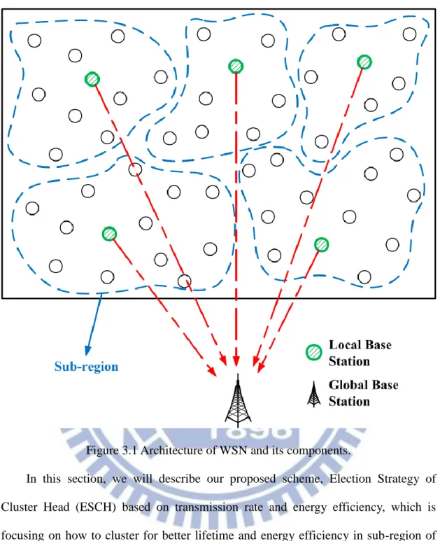
Because the coverage area of WSN may cover several square kilometers, it is impractical for deploying such WSN while the costs of communication and hardware design are difficult to save. To solve the problem of the cost, we focus on the sub-regions which are obtained by dividing the coverage area of WSN. For each sub-region, there are a large number of sensors and one local base station collecting the sensed data which are aggregated and transmitted to the global base station. As shown in Figure 3.1, there is one local base station in each sub-region and the local base station is responsible for receiving the sensed data in the sub-region and transmitting the received data to the global station. Besides, each WSN is corresponding to its only one global base station. The main job of global base station is that receives the data from local base stations for whole WSN. Thus, the primary difference between local and global base station is that the local base station is responsible for the sub-region that it locates in while the global base station has the responsibility for whole WSN. In each sub-region, there are still many sensors, and we can make use of clustering technique to cluster these sensor nodes. After establishing the clusters, the cluster heads send their collected data to the local base station, and then the local base station send the data up to the global base station.

15

Figure 3.1 Architecture of WSN and its components.

In this section, we will describe our proposed scheme, Election Strategy of Cluster Head (ESCH) based on transmission rate and energy efficiency, which is focusing on how to cluster for better lifetime and energy efficiency in sub-region of the WSN.

3.1 Network Model

In this thesis, we make some assumptions for simulating LEACH and ESCH.  The sub-region is assumed to be a square field with M*M square meters, and

there are N sensor nodes which are evenly distributed within the field.

16

of the node. The same capability means that the nodes have similar initial energy and bandwidth.

 All the sensor nodes are static or with low mobility.

 Initially, none of the sensor nodes have information about others.

 Each sensor node can communicate with each other in the field which it belongs to.

 Assuming that nodes sense and collect data continually, they send data during their allocated TDMA time slot.

3.2

ESCH

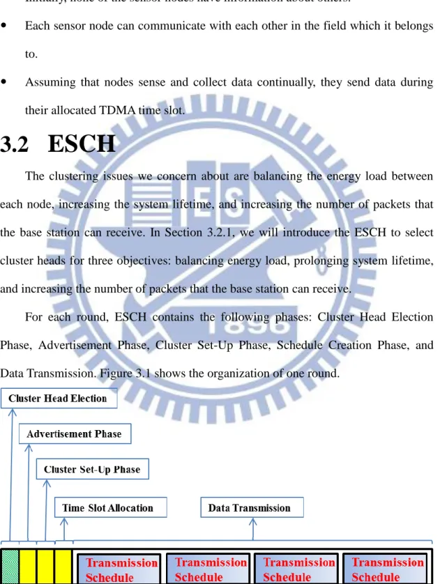
The clustering issues we concern about are balancing the energy load between each node, increasing the system lifetime, and increasing the number of packets that the base station can receive. In Section 3.2.1, we will introduce the ESCH to select cluster heads for three objectives: balancing energy load, prolonging system lifetime, and increasing the number of packets that the base station can receive.

For each round, ESCH contains the following phases: Cluster Head Election Phase, Advertisement Phase, Cluster Set-Up Phase, Schedule Creation Phase, and Data Transmission. Figure 3.1 shows the organization of one round.

17

3.2.1

Cluster Head Election Phase

To elect appropriate cluster heads, each node must know about other nodes information, such as original energy, current energy, and bandwidth. .So, at the beginning of Cluster Head Election Phase, every node checks it remaining energy whether the current energy is below the threshold of becoming a cluster head. If the node remains lots amount of energy, then broadcasts its own three conditions to others. The broadcasted packets with packet type NODE_INFO must contain raw energy, current remaining energy, and bandwidth in the first round.

After the node received the broadcasted packets from other sensor nodes, it fetches the Node’s ID, bandwidth, raw energy, and current remaining energy from a received packet with packet type NODE_INFO and dynamically allocates an entry to place the fetching information. Figure 3.2 shows the data structure of an entry. After receiving packets and fetching the information to store in an entry, there exists a table in which each entry has four fields for storing node ID, bandwidth, current remaining energy, and raw energy, which are coming from the packet with type NODE_INFO, as shown in Figure 3.2.

18

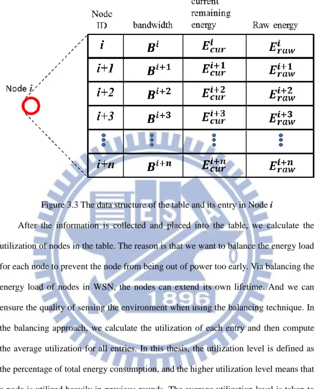
Figure 3.3 The data structure of the table and its entry in Node i

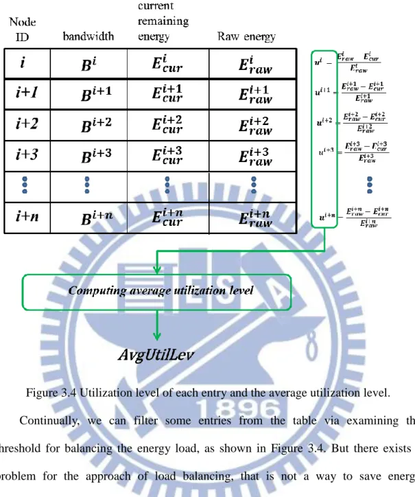
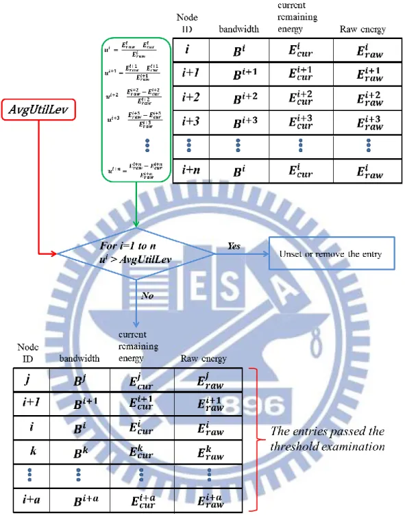
After the information is collected and placed into the table, we calculate the utilization of nodes in the table. The reason is that we want to balance the energy load for each node to prevent the node from being out of power too early. Via balancing the energy load of nodes in WSN, the nodes can extend its own lifetime. And we can ensure the quality of sensing the environment when using the balancing technique. In the balancing approach, we calculate the utilization of each entry and then compute the average utilization for all entries. In this thesis, the utilization level is defined as the percentage of total energy consumption, and the higher utilization level means that a node is utilized heavily in previous rounds. The average utilization level is taken to be a threshold to determine whether the node is heavily utilized. If the utilization level is lower than the threshold, it means that the node was lightly utilized in the past, and it is appropriate in this round to be a candidate for being elected as a cluster head. Figure 3.3 shows the calculation of utilization level and average utilization level as the threshold.

19

Figure 3.4 Utilization level of each entry and the average utilization level. Continually, we can filter some entries from the table via examining the threshold for balancing the energy load, as shown in Figure 3.4. But there exists a problem for the approach of load balancing, that is not a way to save energy effectively. Because the load balancing is a special case in LEACH, it means that the LEACH can have probability to achieve the same selected cluster heads and the number of cluster heads comparing with load balancing approach. The reason is that we only modified the cluster head election to avoid the node draining its energy quickly. Furthermore, in LEACH, it doesn’t take any constraint on electing cluster head and it also doesn’t define the number of cluster heads in each round, so every node has chance to become a cluster head node. We can imagine that for the same WSN using two cluster head elections: the load balancing approach and LEACH. For

20

instance, the cluster heads that are selected in first round by balancing approach are the same comparing with LEACH. In the second round, the LEACH will select the same cluster heads that the balancing approach selects to balance the energy. In a similar way, the condition will happen in the next round, and so on. If we don’t consider any factor that affects the network performance, theoretically, the result after the WSN expiring will be the same in both algorithms. As a result of above reasons, we need a way to save the energy effectively.

21

Figure 3.5 Threshold examination.

We propose a way to save energy while controlling the number of cluster heads in each round. Controlling the number of cluster heads is an effective way to save energy. In LEACH, it doesn’t control the number of cluster head in each round, so it may encounter some problems for saving energy. If the number of cluster is small in the current round, this makes the non-cluster-head consuming more transmission

22

power to transmit packets. When increasing the cluster-head nodes in the current round, the non-cluster-head nodes can have more choices to choose better cluster-head, and thus the distance of communicating to cluster head can be shortened to save transmission power. But if there are too many cluster heads in the current round, it is not effective to save energy because communicating to the base station directly features high power consumption. Although we shorten the communication distance between cluster-head and non-cluster-head nodes, there may be too many cluster heads to communicate to the base station.

In LEACH, via experiment, the best number of cluster heads account for five percent of the total number of nodes. The value CH which is the best number of cluster heads in each round is used in our proposed ESCH for saving energy. After examining the threshold for each entry, we need to determine the number of cluster heads in this round. The number of cluster heads in the current round is obtained by the number of total remaining nodes multiplying by the best number of cluster heads .The number of cluster heads in the current round is obtained by setting the value to the best number of cluster heads CH. Thus considering the total nodes remaining in sub-region of WSN makes the number of cluster heads adaptive in each round.

From the above steps, we have done the load balancing and energy saving by controlling the number of cluster heads in each round. Now, for raising the throughput of the WSN, we rank these candidates that passed balancing threshold examination in descending order based on bandwidth. Then, we select the top CH entries in the table to be cluster heads for the current round. If the current node’s ID is matching with one of the top CH entries of the table, the current node elects itself to become a cluster head in this round, and it goes into the Advertisement Phase. Otherwise, the current node can be non-cluster-head node in this round, and waits for advertisements from

23

the cluster heads. As shown in Figure 3.5, it ranks the entries of the table in descendent order by bandwidth and selects the top of the best number of cluster heads to be cluster heads. Then the node fetches the node IDs of top CH entries from the table after ranking. If one of these IDs that we fetched from the table is the same as the node’s ID, the node elects itself to be a cluster head because it knows that it has sufficient capabilities to become cluster-head node.

24

One of our objectives is to raise the throughput by choosing the nodes with higher bandwidth to be cluster head. Because the cluster head plays a role of transmitting the collected data to the base station, the cluster-head node with higher bandwidth can complete the data transmission faster than those cluster heads with lower bandwidth. As a result, the number of packets received at the base station would be increased.

3.2.2

Advertisement Phase

After the Cluster-head nodes are created in Cluster Head Election Phase, they begin to broadcast an advertisement messages which contains the ID of the cluster head, and packet type (ADV_CH). The advertisement message is broadcasted to the rest of the non-cluster-head nodes. After the non-cluster-head nodes received advertisement messages from cluster-head nodes, each non-cluster-head node selects its cluster head and the cluster it belongs to for this round.

The decision of cluster head for non-cluster-head node is based on the received signal strength index (RSSI) of the advertisement message. The cluster-head advertisement with largest signal strength is selected to be cluster head of the non-cluster-head node. It means that the minimum transmit power is required for communication with the selected cluster head.

For the assumption of ESCH, the advertisement phase may not be needed. Because we assume that each sub-region is independent for clustering, and there are no interferences between sub-regions. This is ideal case in our proposed scheme, but in practical, this phase is needed because we can’t ensure that the nodes in the same sub-region receive the same broadcasting election information. The nodes may receive broadcasting electing information from nodes of other sub-regions, which leads to the tables are different between nodes in the same sub-region.

25

3.2.3

Cluster Set-Up Phase

After each node selecting the preferred cluster to participate in and setting its cluster head, it must send request message to its cluster head for becoming a member of the cluster. The request message for joining a cluster contains the node ID and packet type (JOIN_REQ).

The cluster-head node recognizes the type of the packet it received. If the type of the packet equals to JOIN_REQ, the cluster-head node adds the nodes to the list of the cluster member.

3.2.4

Schedule Creation Phase

After each node joining its cluster, the cluster head needs to create a TDMA schedule that is used to tell the cluster members when it should send its sensed data to its cluster head. This TDMA schedule is broadcasted to the member nodes in the cluster. The packet of TDMA schedule contains the schedule and packet type (ADV_SCH).

In heterogeneous WSN, because different cluster heads have different bandwidth, the time for cluster head transmitting data to the base station varies. With higher bandwidth in the cluster head, the slot length of TDMA can be reduced because the higher bandwidth makes the transmission time to the base station short. In addition, the more TDMA schedules can fit in the phase of data transmission, and thus more sensed data packet can be received at the base station.

3.2.5

Data Transmission

Once the non-cluster-head nodes receive the TDMA schedule from its cluster head, and the data transmission starts. The type of data packet is DATA that is used to identify the cluster-head node and the base station. Each node that has received the schedule knows when to transmit its sensed data. So the radio of non-cluster-head

26

nodes can be turned off until the time that it is allowed to transmit. This way can avoid idle listening to save the energy of the nodes and the non-cluster-head node can go into sleep mode to save more energy.

Figure 3.7 Data Transmission time line

3.2.6

Re-Clustering

Re-clustering is needed for every round. Each non-cluster-head node in a round not only senses the environment but also transmits the sensed data to the cluster head which it belongs to. Moreover, the cluster-head nodes have an extra job to receive sensed data from their members and transmit the aggregated data to the base station.

As described above, both non-cluster head nodes and cluster-head nodes consume their energy in sensing and transmission. In addition, the cluster heads need to spend energy to receive from member nodes. Since the cluster-head nodes have more work to do, the rate of energy consumption is usually faster than non-cluster head nodes.

Because the workload of each node is different, the amount of energy that is consumed by the nodes will be diverse. In a round, the node may consume lots of energy or may be dead, so it is not appropriate to serve as a cluster head. Thus, re-clustering is required at the beginning of each round to avoid node’s energy being consumed too much and adjust the number of cluster heads as we preferred.

27

After the first round of ESCH, each node in the same sub-region has a table recording other’s bandwidth and raw energy values, because these values are constant for sensor nodes. So for saving more energy in WSN, the nodes can just broadcast current remaining energy to others when in electing information collection state.

3.2.7

Overview of ESCH

28

Chapter 4 Simulation and Results

4.1 Simulation Environment

In order to evaluating the performance of our ESCH in a sub-region of the heterogeneous WSN, we use the network simulation tool ns-2 [10]. To simplify the simulation, we set the area of the simulation to square. The initial simulation parameters that we used in the ESCH and LEACH are shown in Table 4.1.

Parameter Value

Simulation Area 100 x 100 m2

Number of total nodes (Ntotal) 100

Number of CH (5 % of Ntotal) 5

Round time 20 seconds

The terminate condition for simulation 1. Ntotal < 5

Eelec 50 nJ/bit

EDA 5 nJ/bit

d0 87.7 m

εfs (d ≤ d0) 10 pJ/bit/m2

εmp (d > d0) 0.0013 pJ/bit/m4

Table 4.1 The initial parameters for simulation.

29

to the initial setting of energy and bandwidth. Actually, after running the simulation we can’t accurately classify the sensor nodes because the remaining energy of each node is varying. In Table 4.2, it lists the initial setting of each node and classifies them according to their initial capabilities.

Type 1 Quantity: 70 Energy: 2 J Bandwidth: 1 Mbps Type 2 Quantity: 12 Energy: 4 J Bandwidth: 3 Mbps Type 3 Quantity: 9 Energy: 6 J Bandwidth: 5 Mbps Type 4 Quantity: 6 Energy: 8 J Bandwidth: 7 Mbps Type 5 Quantity: 3 Energy: 10 J Bandwidth: 9 Mbps Table 4.2 The setting of nodes for each type

4.2 Metrics of Performance

The metrics of performance for WSN is introduced in this section. These metrics are network lifetime, energy consumption, the number of packet received, and the number of cluster heads in each round.

30

The network lifetime is defined as the period of time from the beginning of the operation of WSN to the time that satisfies the terminate condition. The network lifetime can be evaluated in different ways [11]:

 First Node Dead (FND)  Half Node Dead (HND)  Last Node Dead (LND)

If we are focusing on the quality of services, FND may be a better choice than LND to estimate the performance.

 Energy Consumption: the amount of energy consumption is the sum of the energy consumption at each node in the WSN. The lower energy consumption in one round means that the whole WSN took less energy to transmit and receive the sensed data. The energy consumption at the base station is not taken into account.

 Number of Packet Received: This metric is evaluated as the number of packets received at the base station. It is defined that in a round how many effective packets that the base station can receive from the cluster heads in WSN. In a round, the more packets the base station receives, the better is the throughput for the WSN.

 Number of Cluster Head: The number of cluster head in each round will affect both energy consumption and the number of packet received. If there are too many cluster-head nodes in the WSN, a large number of cluster heads will have to communicate with the base station directly. Because the cluster-head nodes are usually far away from the base station, the energy consumed for data transmission will increase. On the other hand, the fewer cluster-head nodes, the number of members in the cluster will increase. This condition makes the cluster-head nodes need to spend more energy on

31

receiving. And non-cluster-head nodes may consume their energy quickly because the distances of the non-cluster-head nodes may become large. This makes the total energy consumption of WSN increase. Anyway, the number of cluster heads affects the energy consumption in a round.

4.3 Simulation Results Analysis

4.3.1

Lifetime

In Table 4.3, it shows that our proposed ESCH is 23.1 % better than LEACH for the time of FND. And the time of HND in ESCH is 12.1 % better than that in LEACH.

The time of FND and HND in ESCH are longer than LEACH, because the ESCH adopts the manner that balances the energy load of each node. At the beginning of ESCH, we examine the utilization level which means the amount of energy consumption in term of how much percentage of original energy in the node. The indicator of energy balancing is the utilization level, which points out how much energy of the node is utilized from the beginning until now.

FND HND LND

LEACH (seconds) 405 630 1070

ESCH (seconds) 527 990 1200

Performance 23.1 % 57.1 % 12.1 %

Table 4.3 The time comparison for FND, HND and LND.

From Figure 4.1, at the same time, the number of the nodes surviving in ESCH is more than that in LEACH. Since the cluster head selection of LEACH doesn’t take the residual energy into account, the node with little energy may become cluster head which results in heavy energy consumption, and the node would die quickly. But the

32

node with higher energy can’t represent any meaning, thus we pay attention on utilization while considering the original energy of each node. So, we can select the less utilized node to be cluster head to distribute energy load to avoid overusing on the node with high energy.

Figure 4.1 also shows that the lifetime of ESCH is longer than LEACH. The factor of prolonging the system lifetime is adapting the number cluster head according to the number of nodes surviving in a sub-region. After some nodes were dead, the number of cluster head in most of rounds is more than ESCH because the less number of nodes will increase the probability to be cluster head in the current round. So, if the number of cluster heads is larger than the best number of cluster heads, the energy consumption will increase. In ESCH, we use the best number of cluster heads to be a reference for the number of cluster-heads in the current round. Also, the less number of cluster heads will increase energy waste since the communication distance between the cluster head and its members may become larger so as to increase transmission power. However, using the adaptive control of the number of cluster heads can reduce the consumption of energy.

33

Figure 4.1 Number of alive nodes over time.

4.3.2

Energy Consumption

Figure 4.2 shows the energy consumption over simulation time. In Figure 4.1, we can see the gap of LEACH and ESCH is obvious for number of alive nodes at 500 second. The number of nodes which survives will be the factor that affects the number of cluster head in LEACH so that the energy consumption is also influenced. The details about energy consumption that we will discussed in later paragraphs.

Before 500 second, the diversities of energy consumption in LEACH and ESCH are almost the same. There are some factors for this result. One is that the ESCH have more probabilities to elect the cluster heads with higher bandwidth so the energy consumption will be higher. At the same time, we also control the number of cluster heads to the best one, and it can save power for communications with the nodes and

34

base station. Another factor is that the LEACH randomly selects the nodes to be cluster heads that doesn’t consider the bandwidth, so the energy consumption is usually lower than ESCH. But the number of cluster heads is not managed by LEACH, the energy consumption can be higher when the number of cluster heads is not equal to the best one. Since the different factors for increasing or decreasing energy consumption affect each other, the energy consumption for both strategies are almost the same before 500 second.

After 500 seconds, we can compare Figure 4.1 and Figure 4.2. In Figure 4.1, after 500 seconds, the nodes surviving are decreasing, and the energy consumption is raised. When the number of nodes decreases in LEACH, the total energy consumption will increase. One reason is that the number of cluster head may be raised due to the increasing probabilities of selecting cluster head. Another factor is that the number of members in a cluster is reduced, and thus the length of TDMA schedule will be shortened. Because a shorter TDMA schedule can place more transmissions than long TDMA schedule for transmission phase, the data transmission of sensed data will increase so that the energy consumption is raised. In ESCH, because of the energy balancing and adapting the number of cluster heads, the energy consumption is lower and much stable than LEACH.

35

Figure 4.2 Total energy consumption over time

4.3.3

Number of Packet Received

From the observation of Figure 4.3, the number of packets that the base station received in ESCH is always better than that in LEACH. The factor is that the LEACH election strategy never takes the bandwidth of the node into account, so for the same period of time the LEACH can’t achieve the same performance of ESCH. In contrast to the election strategy of LEACH, the ESCH selects the top CH of nodes with higher bandwidth after filtering the node by utilization level checking. Once the cluster is created, the transmission time for transmitting data to the base station can be reduced and thus the TDMA schedule is shorten. This makes the TDMA schedule have more probability to fit more schedules into the data transmission phase, so the number of packets received at the base station can be raised.

36

Figure 4.3 Number of packets received at BS over time.

The Figure 4.4 shows the relationship of energy consumption and the number of received packets at the base station. For the same energy consumption, ESCH performs better than LEACH. The reason is that ESCH adopts the method of adapting cluster head to save energy for communications, and selects the higher bandwidth to make the cluster heads transmit more sensed data to the base station.

37

Figure 4.4 Energy versus Number of Received Packets at BS

4.3.4

Number of Cluster Head

The ESCH controls the number of cluster heads to avoid the energy depleting quickly. If too many cluster heads exist in the sub-region of WSN and these cluster heads communicate directly with the base station, since the base station is usually far away from the cluster heads, it causes the cluster heads to raise its transmission power for communicating with the base station. If too few cluster heads exist in the sub-region, we still can’t get the benefit for energy saving. This is because the communication distance between cluster members and the cluster head is raised since there are too few cluster heads to make a good choice. Because the transmission power is proportional to square of the distance, the energy depletion for communication within a cluster needs to be concerned.

38

From Figure 4.5, the ESCH has a stable number of cluster head. In contrast to ESCH, the number of cluster head in LEACH is varying. The reason is that LEACH doesn’t consider controlling the number of cluster head. By observing Figure 4.1, after 600 seconds, the number of surviving node in LEACH is decreasing but the number of cluster head may be bigger than the best number of cluster heads. In ESCH, it adapts the number of cluster head according to the number of node existing in a sub-region. So, the number of cluster heads decreases as the number of surviving node drops. Through this way we can save the energy on communications, no matter within the cluster or from the cluster head to the base station.

39

Chapter 5 Conclusions and Future

Works

In this thesis, we presented an election strategy of cluster-head nodes. First, to balance the load of energy, we check the utilization level of each node. While the current node passes the examination of utilization level threshold, it is capable to compete with other candidate nodes. Next, the ESCH adapts the number of cluster head to save energy for communications. The ESCH sets the number of cluster head to the best one in the current round. Finally, each node shows its own bandwidth to decide who can become a cluster head. By ranking their bandwidth in descendent order, and choose the best of CH nodes which is the number of cluster head calculated from the last step, the base station can always receive more packets than LEACH. And because of distributing energy load, the number of nodes surviving in ESCH is more than that in LEACH. Furthermore, the ESCH saves more energy than LEACH via controlling the number of cluster heads in each round.

In this work, he best number of cluster head that ESCH adopted is from the experiment of LEACH. This optimal value is based on the homogeneous WSN, but it may not be optimal in the heterogeneous WSN. Because the diversities of bandwidth in heterogeneous WSN, the rate for energy depletion is much different from that in homogeneous WSN. Thus, we can take the rate of energy depletion into account to obtain the optimal number of cluster heads in the future work.

While the ESCH is focusing on a sub-region of whole WSN, the further work is how to select a local base station that is responsible for transmit sensed data to the global base station in this sub-region.

40

References

[1] I. F. Akyildiz, W. Su, Y. Sankarasubramaniam, and E. Cayirci, “Wireless sensor networks: a survey,” Computer Networks, Volume 38, Issue 4, pp. 393-422, March 2002.

[2] J. Yick, B. Mukherjee, and D. Ghosal, “Wireless sensor network survey,” Computer Networks, Volume 52, Issue 12, pp. 2292-2330, August 2008.

[3] K. Akkaya and M. Younis, “A survey on routing protocols for wireless sensor networks,” Computer Networks, Volume 3, Issue 3, May 2005.

[4] W.R. Heinzelman, A. Chandrakasan and H. Balakrishnam, “Energy-Efficient Communication Protocol for Wireless Microsensor Networks,” HICSS '00 Proceedings of the 33rd Hawaii International Conference on System Sciences, Jan 2000.

[5] V. Mhatre and C. Rosenberg, “Homogeneous vs Heterogeneous Clustered Sensor Networks: A Comparative Study,” IEEE International Conference on Communication, Volume 6, pp. 3646-3651, June 2004.

[6] V. Katiyar, N. Chand, and S. Soni, “Clustering Algorithms for Heterogeneous Wireless Sensor Network: A Survey,” International Journal of Applied Engineering Research (IJAER), Volume 1, No 2, 2010.

[7] W.B. Heinzelman, A. Chandrakasan and H. Balakrishnan, “Energy-Efficient Communication Protocol for Wireless Microsensor networks,” Proceedings of the 33rd Annual Hawaii International Conference on System Services, Jan 2000.

[8] W.B. Heinzelman, A. Chandrakasan, and H. Balakrishnan, “An Application-Specific Protocol Architecture for Wireless Micorsensor Networks,” IEEE Transaction on Wireless Communications, Volume 1, Issue 4, Oct 2002.

41

wireless sensor networks,” International Journal on Computer Science and Engineering (IJCSE), Volume 02, No. 08, pp. 2633-2640, 2010

[10] The Network Simulator ns-2. [ online ]. Available: http://www.isi.edu/nsnam/ns/ [11] M. Handy, M. Haase, and D. Timmermann, “Low Energy Adaptive Clustering Hierarchy with Deterministic Cluster-Head Selection,” 4th International Workshop on Mobile and Wireless Communications Network, pp. 368-372, 2002.

[12] G. Smaragdakis, I. Matta, A. Bestavros, “SEP: A Stable Election Protocol for clustered heterogeneous wireless sensor networks”, Second International Workshop on Sensor and Actor Network Protocols and Applications (SANPA 2004), 2004. [13] Z. Hong, L Yu, G. Zhang, “Efficient and Dynamic Clustering Scheme for Heterogeneous Multi-level Wireless Sensor Networks”, Acta Automatica Sinica, Volume 39, Issue 4, pp. 454-460, April 2013.

[14] J. Peng, T. Liu, H. Li, B. Guo, “Energy-Efficient Prediction Clustering Algorithm for Multilevel Heterogeneous Wireless Sensor Networks”, International Journal of Distributed Sensor Networks, Jan 2013.