在行動無線感測網路下基於色彩理論之動態定位技術

全文

(1)國立交通大學資訊科學系碩士論文. 在行動無線感測網路下基於色彩理論之動態定位技術. Color-theory-based Dynamic Localization in Mobile Wireless Sensor Networks. 研究生：施勝海指導教授：王國禎. 博士. 中華民國九十四年六月.

(2) ii.

(3) 在行動無線感測網路下基於色彩理論之動態定位技術. Color-theory-based Dynamic Localization in Mobile Wireless Sensor Networks 研究生：施勝海. Student：Shen-Hai Shee. 指導教授：王國禎. Advisor：Kuochen Wang. 國立交通大學資訊科學系碩士論文 A Thesis Submitted to Department of Computer and Information Science College of Electrical Engineering and Computer Science National Chiao Tung University in Partial Fulfillment of the Requirements for the Degree of Master in Computer and Information Science June 2005 Hsinchu, Taiwan, Republic of China. 中華民國九十四年六月 i.

(4) i.

(5) ii.

(6) iii.

(7) iv.

(8) v.

(9) vi.

(10) 在行動無線感測網路下基於色彩理論之動態定位技術. 學生：施勝海. 指導教授：王國禎博士. 國立交通大學資訊科學系. 摘要定位資訊在無線感測網路的應用中扮演了很重要的角色。例如，利用定位的資訊，路由的進行可以更加有效率。由於 GPS 的價格昂貴，所以現有的定位方法是利用網路中少許具有定位功能的節點幫助其他節點作定位的工作，但是現有的方法中卻很少探討節點可移動之情況。在這一篇論文中，我們提出了一個基於色彩理論的行動定位演算法，CDL。CDL 利用網路中全部的參考點資訊，如其位置以及 RGB 值資訊，以幫助伺服器建立一個位置資料庫及協助每一個節點計算出其 RGB 值，接下來每個節點的 RGB 值會傳送至伺服器端來做定位的工作。因為 CDL 是採取集中式的架構，所以適合應用於需要伺服器做監控或是收集資訊的環境，例如社區照護系統或是醫療監視系統。 ii.

(11) 我們的評估結果顯示，與另一個在行動感測網路環境下的定位方法 MCL 相較，CDL 的平均定位準確度比 MCL 好約 40% - 50%。關鍵詞：色彩理論、動態定位、行動無線感測網路 `. iii.

(12) Color-theory-based Dynamic Localization in Mobile Wireless Sensor Networks Student：Shen-Hai Shee. Advisor：Dr. Kuochen Wang. Department of Computer and Information Science National Chiao Tung University. Abstract Location information is critical to wireless sensor network (WSN) applications. With the help of location information, for example, routing can be performed more efficiently. Since the GPS receiver is expensive, existing localization approaches use a small number of seed nodes that are aware of their locations to help estimate the locations of other sensor nodes in fixed WSNs. However, there are few schemes involved mobility of sensor nodes. In this thesis, we propose a novel localization approach, Color-theory based Dynamic Localization (CDL), which is based on color theory to exploit mobile positioning in mobile WSNs. CDL makes use of the broadcast information from all seed nodes, such as their locations and RGB values to help the server to create a location database and assist each sensor node to compute its RGB values. Then, the RGB values of all sensor nodes are sent to the server for localization of sensor nodes. CDL is easy to implement and is a centralized approach; thus it is very suitable for applications that need a centralized server to collect user data and monitor user activities, such as community health-care systems and hospital monitor systems. Simulation results show that in the MSNs, the location accuracy of CDL is 40% - 50% better than that of MCL [17], which is only available. iii.

(13) location approach targeted for mobile positioning in WSNs so far. Keywords : color theory, dynamic localization, mobile wireless sensor network. iv.

(14) Acknowledgements Many people have helped me with this thesis. I deeply appreciate my thesis advisor, Dr. Kuochen Wang, for his intensive advice and instruction. I would like to thank all the classmates in Mobile Computing and Broadband Networking Laboratory for their invaluable assistance and suggestions. The support by the National Science Council under Grant NSC93-2213-E-009-124 is also grateful acknowledged. Finally, I thank my Father and Mother for their endless love and support.. v.

(15) Contents. Abstract (in Chinese). i. Abstract (in English). iii. Acknowledgements. v. Contents. vi. List of Figures. viii. List of Tables. ix. List of Algorithms. x. Chapter 1. Introduction............................................................................................ 1. Chapter 2. Related Work.......................................................................................... 3. 2.1. 2.2 Chapter 3. Categories of Existing Localization Approaches .................................... 3 2.1.1. Indoor localization systems ...........................................................3. 2.1.2. Outdoor localization systems......................................................... 4. Comparison of Different Localization Approaches ................................ 7 Design Approach .................................................................................... 9. vi.

(16) 3.1. Introduction to Color Theory .................................................................. 9. 3.2. Introduction to CDL.............................................................................. 10. 3.3. The Information Delivery of Seeds....................................................... 12. 3.4. The Establishment of Location Database. ............................................ 13. 3.5. Mobility................................................................................................. 17. Chapter 4. Simulation Results and Discussion ..................................................... 19. 4.1. Simulation Model.................................................................................. 19. 4.2. Comparison with MCL [17].................................................................. 22. Chapter 5. Conclusions and Future Work ............................................................ 26. 5.1. Concluding Remarks............................................................................. 26. 5.2. Future Work .......................................................................................... 26. Bibliography ................................................................................................................. 27. vii.

(17) List of Figures. Fig. 1.The mixture of primary colors...........................................................10 Fig. 2. HSV cone..........................................................................................12 Fig. 3. The CDL algorithm...........................................................................18 Fig. 4. Impact of node density......................................................................21 Fig. 5. Impact of seed density. .....................................................................22 Fig. 6. Accuracy comparison. ......................................................................23 Fig. 7. Impact of node density......................................................................24 Fig. 8. Impact of seed density. .....................................................................25. viii.

(18) List of Tables. Table 1 : Comparison of different localization approaches. ....................................8 Table 2 : Simulation parameters ...........................................................................20. ix.

(19) List of Algorithms Algorithm 1: Procedure for converting RGB to HSV [23]....................................15 Algorithm 2: Procedure for converting HSV to RGB [23]....................................16. x.

(20) Chapter 1 Introduction A wireless sensor network (WSN) consists of a collection of wireless sensor nodes operating in an ad hoc manner within a particular area. Because of the properties of low-powered, small sizes, low-cost, WSNs can be applied to several areas, including battlefields, emergency systems, health-care systems and smart home. For WSNs, localization is a critical issue. By exploiting location information, routing protocols can operate more efficiently. To obtain locations, nodes may be equipped with a GPS receiver, which is considered accurate and reliable; nevertheless, it is expensive and not feasible for sensor nodes due to its power consumption. Existing localization approaches can be divided into two categories roughly: range-based and range-free. In range-based approaches, certain ranging technologies are employed by sensor nodes to measure the distances between nodes, which include Received Signal Strength Indicator (RSSI), Time Difference of Arrival (TDOA), Angle of Arrival (AOA) etc. With the knowledge of distances to at least three location-aware nodes or seeds, nodes are able to calculate their locations by performing triangulation. In range-free approaches, localization is performed without the need of ranging hardware; thus they are more cost-efficient and consume less energy. But as it should be, they are coarser in terms of location accuracy.. 1.

(21) For the design of localization approaches for mobile MSNs, mobility presents a critical issue. Lots of localization approaches are presented [2] [3][12][14]. However, few of them deal with mobile localization for mobile WSNs. There are a few mobility issues addressed. [4] discussed the issue of mobility prediction in WSNs. With the help of the prediction of mobility, the connectivity failure can be predicted and prevented. In [5], mobility is taken into account to the effect of localization. In [1], four mobile beacons are used to form a square and nodes within their center of detection area calculate their corresponding locations as the centroid of the square. The thesis is organized as follows. In Chapter 2, the related work of localization is reviewed. In Chapter 3, the design approach is proposed. Simulation of the design approach is performed and discussed in Chapter 4. Finally, conclusions remarks are given and future work is outlined in Chapter 5.. 2.

(22) Chapter 2 Related Work In this chapter, we review existing localization approaches and compare them qualitatively.. 2.1 Categories of Existing Localization Approaches Because of the diverse properties of environments and signals used, existing localization methods are classified into indoor and outdoor localization systems.. 2.1.1 Indoor localization systems The design and deployment of indoor localization systems are challenge tasks due to the indoor characteristics. With the existence of metal and reflective materials that influence the propagation of signals and cause multipath effects and interference, the way of designing indoor localization systems is completely different from that of outdoor localization systems. However, on the other point of view, the in-building localization system can exploit the spatial properties of the region to promote efficiency and accuracy. In [6], a predictive model for indoor tracking of mobile users was proposed The building is segmented into several spatial components and the trajectory of the users is represented by an abstract spatial graph. In addition to the conventional localization system that tracks users using signal strength and direction [10], the properties of the location fingerprint were employed to improve the design and the deployment of the localization algorithms [7][8]. In RADAR[7], the signal data of various locations are collected and recorded as a function of the user location. 3.

(23) The database stores the collected signal data, which is known as location fingerprint database, which is a critical step in the design of location algorithms. The properties of signal should be taken into consideration carefully [8]. An analytical model was proposed to analyze indoor positioning system [9].. 2.1.2 Outdoor localization systems Outdoor localization systems are featured in large-scale, hop-by-hop transmitting, and small number of seeds, and can be classified according to mobility of networks.. 2.1.2.1 Static localization system Ad hoc positioning system [11]: The Ad Hoc Positioning System (APS) uses one of several propagation methods to perform localization. The hop-by-hop propagation approach is used to obtain the distances between the nodes and landmarks. Once an arbitrary node has obtained distances to more than 3 landmarks, it is able to perform triangulation to estimate its location. There are three propagation methods proposed: DV-hop, DV-distance and Euclidean propagation methods. DV-hop employs a distance vector exchange so that each node obtains the hop distances to the reference nodes. It is simple and only works for isotropic networks. DV-distance is similar to DV-hop; however, the distance between nodes is measured using ranging technologies. Euclidean propagation method is based on propagating the euclidean distance to reference nodes. The drawback of APS is that the topology of APS needs to be regular or symmetrical. Besides, the high density of landmarks is needed to guarantee certain accuracy. Multidimensional scaling [3]: The multidimensional scaling (MDS) determines the relative locations of nodes by using local distance information and MDS-MAP [26]. With few seeds, the performance of MDS is still good even within anisotropic 4.

(24) topologies and complex regions. The disadvantages of MDS are high computation complexity and poor scalability. Localization of wireless sensor networks with a mobile beacon [14]: This approach exploited a mobile beacon to perform localization. Each node receiving packets from a mobile beacon uses the information including the coordination of the beacon to estimate its location and infer the location constraints to the mobile beacon. Each node applies Bayesian inference to calculate its new position from its old estimated position. After receiving all of the packets from the mobile beacon, the final position estimate is computed. It is cost effective and simple because only a beacon is needed. The drawback is that it lacks of robustness. In other words, the system would crack down if the mobile beacon collapses. Moreover, it is necessary for the mobile beacon to have full energy. Location estimation system using wireless ad hoc networks [13]: The system uses an accumulator host to perform localization. Sensor nodes measure distances to their neighbors and elect a host among them as an accumulator host. The mission of the accumulator host is gathering estimated distances from other sensor nodes and estimates the locations of them. Because of the way of gathering information, it lacks of scalability. In addition, the overhead of the system is expected to soar substantially when the number of sensor nodes increases. Others: [1] performed localization using mobile beacons, which is different from [14]. In [1], the algorithm is based on only one mobile beacon which is aware of its position by equipping a GPS receiver. The sensor nodes estimate their locations by using receiving packets including the beacon’s location information delivering by the mobile beacon. In [1], four mobile beacons move towards the node to be localized and. 5.

(25) form a square. The location of the sensor node is the centroid of the four mobile beacons’ locations. The comparison of localization algorithms for sensor networks with only one mobile beacon is given in [15]. The mobile-beacon algorithms are characterized by its simplicity of implementation and flexibility. However, the robustness is a critical problem with the concern of the failure of the mobile beacons.. 2.1.2.2 Mobile localization systems There are few existing localization algorithms in which mobility is involved. Nevertheless, mobile networks play an important role in the field of wireless networks. Most concerns were focused on the influence of mobility upon wireless sensor networks. [16] uses node position and speed to predict when partitioning will occur and which link is critical. [4] predicts the change of network topology by exploiting the regularity in mobility patterns and thus improves existing routing protocols. GPS-less low-cost outdoor localization for very small devices [12]: The centroid method assumes that the ranges of coverage of reference points overlap with each other. With the assumption, each node uses the connectivity metric to get a subset of reference nodes and localizes it to the centroid of the selected reference nodes. While the method is simple and requires no coordination among sensor nodes, its application is limited due to the assumption of overlapping coverage of the reference points. Localization for mobile sensor networks (MCL) [17]: In this approach, sequential Monte Carlo method is used to estimate the posterior distribution of discrete time dynamic models. There are two phases involved, which are prediction and filtering. In the prediction step, a node computes its possible location by applying the mobility model to each sample. In the filtering step, a node filters possible locations based on new observations. Besides, it is a range-free algorithm which is cost effective but is. 6.

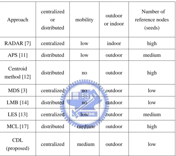
(26) less accuracy than the range-based approach. The MCL needs high seed density to improve location accuracy during the exploitation of seeds in the filtering phase. Mobility-enhanced positioning in ad hoc networks (MAP) [24]: In MAP, mobility is concerned and the simulation showed the performance was improved with the aid of mobility. The simulation results have shown that mobile nodes can improve accuracy by bridging gaps within neighborhoods.. 2.2 Comparison of Different Localization Approaches The above mentioned approaches are compared in Table 1, according to the following factors: centralized or distributed, mobility, outdoor or indoor and number of reference nodes. The proposed color-theory based dynamic localization (CDL) is also included in the table, which will be described in Chapter 3. First, the metric of centralized or distribued indicates that whether there is a server in the network responsible for localization of all nodes or not. In APS, Centroid method, LMB and MCL, nodes perform localization locally; the other approaches rely on a server to perform localization. Secondly, mobility indicates weather nodes in network are fixed or mobile. MCL exploits mobility of nodes to improve location accuracy. Thirdly, the outdoor or indoor metric is related to the environment of networks. Only the RADAR is performed indoor. Fourthly, the number of reference nodes is the number of nodes needed in networks. MDS uses distance information among nodes and needs less reference nodes. LMB only involves one mobile beacon to deliver location information. Each node in CDL does localization using information of all reference nodes and thus it performs well with few reference nodes.. 7.

(27) Table 1 : Comparison of different localization approaches.. Approach. centralized or distributed. mobility. outdoor or indoor. Number of reference nodes (seeds). RADAR [7]. centralized. low. indoor. high. APS [11]. distributed. low. outdoor. medium. Centroid method [12]. distributed. no. outdoor. high. MDS [3]. centralized. no. outdoor. low. LMB [14]. distributed. no. outdoor. low. LES [13]. centralized. low. outdoor. medium. MCL [17]. distributed. medium. outdoor. high. CDL (proposed). centralized. medium. outdoor. low. 8.

(28) Chapter 3 Design Approach In this chapter, we propose a novel color-theory-based dynamic localization (CDL) algorithm. We first introduce the color theory, and then the proposed localization algorithm is described.. 3.1 Introduction to Color theory Consider what happens if we mix blue and yellow color together. The result will be the green color. In the color model, the red, green and blue are the three additive primaries. Any color can be obtained by mixing together various amounts of red, green and blue colors. If the color primaries, red, green, blue are mixed, they may form the yellow, cyan, magenta, and yellow [18]. When all three primaries overlap, they produce white, as shown in Fig. 1.. 9.

(29) Green Cyan. Yellow White Red. Fig. 1.. Magenta Blue. The mixture of primary colors. The three colors, green, red, and blue, are mixed and produce. yellow, white, magenta, and cyan.. In the RGB system, every color can be expressed by assigning different values within some scale, for example, 0 to 1. In addition to the RGB system, there exists another color system, HSV. HSV stands for Hue, Saturation, and Value, and it uses these three concepts to describe a color [21]. In the HSV model [22], the hue is depicted as a three-dimensional conical formation of the color wheel. The saturation is represented by the distance from the center of a circular cross-section of the cone, and the value is the distance from the pointed end of the cone, as shown in Fig. 2.. 3.2 Introduction to CDL Since our approach involves both the RGB and HSV systems, the conversion algorithms between HSV and RGB are needed. We adopted the algorithms described in [23]. Our approach is based on the color theory, in which the location of sensor node i is represented as three different values, namely, ( Ri , Gi , Bi ) . A seed is a sensor node aware of its location by equipping a GPS receiver. We adopted the DV-hop. 10.

(30) approach [24] to obtain the distances between nodes. There are four phases involved in the CDL. In the first phase, each seed is assigned with different RGB values and it broadcasts a packet including these values along with its location to its neighbors. The neighbors receiving the packet would record the number of hops to the seed. After completing the broadcast, each seed receives a set of hop count values from all other seeds and is able to calculate the distances and hops to all other seeds. The total distance and total hop count values to all other seeds are computed and propagated through all nodes in the WSNs. Upon obtaining the information from all seeds, each node computes the average hop distance [24]. In the second phase, once the nodes nearby the seeds receive the RGB values and locations from seeds, they convert the RGB values to corresponding HSV values by an algorithm RGBtoHSV [23].. Based. on the color theory, the lightness of color fades out with the increasing of propagating distances. The V of HSV of a seed, which is corresponding to the lightness, is decreased in proportion to the hop distance to the seed . With the new HSV values, the corresponding RGB values are obtained by using another algorithm, HSVtoRGB [23] . In the third phase, the task of transforming RGB values into a location is performed by a server. By the means of broadcasting, the RGB values of each seed along with its location would be received by the server eventually, and thus topology of all seeds is obtained as well. A location database is then constructed by the server. In the fourth phase, the RGB values of sensor nodes are transmitted to the server, which will calculate the current location of each sensor node. The detail of the proposed algorithm is described as follows.. 11.

(31) V (0 to 1). Green. Magenta Blue. H (0 to 360 ) S (0 to 1) Black Fig. 2. HSV cone.. 3.3 The Information Delivery of Seeds In this section, we first define some notations for CDL and describe the first phase of the proposed approach, namely, the distribution of the RGB values of seeds to whole sensor nodes. First of all, some notations need to be definited: ¾. Each node i maintains a table of ( Rik , Gik , Bik ) and Dik , k represents the kth. seeds. ¾. Davg is the average distance.. ¾. hij is the hop distance between nodes i and j.. ¾. Dik represents the hop distance from seed k to node i : Dik = Davg × hik. ¾. Range represents the maximum distance that a color can propagate.. ¾. ( Rk , Gk , Bk ) is the RGB value of seed k.. ¾. ( H ik , S ik ,Vik ) is the HSV values of seed k received by the ith node. 12.

(32) The RGB values of seeds are assigned randomly from 0 to 1. After a sensor node obtains each seed’s RGB values and the average distance and hop counts to other seeds, the RGB values are first converted to HSV values by equation (1). ( H k , S k ,Vk ) = RGBtoHSV ( Rk , Gk , Bk ). (1). The updated HSV values corresponding to node i of seed k are calculated by equation (2).. H ik = H k ,. S ik = S k , Vik = (1 −. Dik ) × Vk Range. (2). The RGB values of node i corresponding seed k are then calculated: ( Rik , Gik , Bik ) = HSVtoRGB ( H ik , S ik , Vik ) (3) The RGB values of node i are the mean of the RGB values of all seeds. 1 n ( Ri , Gi , Bi ) = × ∑ ( Rik , Gik , Bik ) n k =1. (4). where n is the number of seeds that node i received. Each seed will broadcast its RGB values and location. With the knowledge of the RGB values and locations of all seeds, the server can construct a location database.. 3.4 The Establishment of Location Database The establishment of a location database is performed when the server obtains the RGB values and coordinates of all seeds. The mechanism is based on the theorem of the mixture of different colors. With the RGB values of all seeds, the RGB values of all locations can be computed by exploiting the ideas of color propagation and the mixture of different colors. In the first place, the distance between every location i and 13.

(33) seed k is obtained:. d ik =. (xi − x k )2 + ( y i −. yk )2. (5). where ( xi , y i ) is the coordinate of location i, and ( xk , y k ) is the location of seed k. First of all, we have to calculate the HSV of every location i corresponding to seed k. ( H k , S k ,Vk ) = RGBtoHSV ( Rk , Gk , Bk ) H ik = H k , S ik = S k , Vik =. d ik • Vk Range. ( Rik , Gik , Bik ) = HSVtoRGB ( H ik , S ik , Vik ). (6) (7) (8). The RGB values of location i: ( Ri , Gi , Bi ) =. 1 N × ∑ ( Rik , Gik , Bik ) N k =1. (9). where N is the number of seeds. In this way, the location for each sensor node can be constructed in the location database by maintaining the coordinate ( x i , y i ) and the RGB values ( Ri , Gi , Bi ) at each location i. The location of a sensor node can be acquired by looking up the location database.. 14.

(34) Procedure: RGBtoHSV ( Red , Green , Blue ) { if Red == 1 and Green == 1 and Blue == 1 { Hue=0; Saturation =0; Value = 1; Return Hue,Saturation,Value; } MINIMUM = Minimum of [ Red, Green, Blue ]; MAXIMUM = Maximum of [ Red, Green, Blue ]); Value = MAXIMUM; Delta = MAXIMUM - MINIMUM; if MAXIMUM != 0 Saturation = Delta / MAXIMUM; else { Red = Green = Blue = 0 Saturation = 0; Hue = -1; } if Red == MAXIMUM Hue = ( Green - Blue ) / Delta; else if Green == MAXIMUM Hue = 2 + ( Blue - Red ) / Delta; else Hue = 4 + ( Red - Green) / Delta; Hue =Hue * 60; if Hue < 0 Hue = Hue+ 360; }. Algorithm 1: Procedure for converting RGB to HSV [23]. 15.

(35) Procedure: HSVtoRGB(Hue , Saturation , Value) {. if Saturation == 0 Red = Green = Blue = Value; Exit ; Hue =Hue/ 60; I = the floor value of Hue; Factorial = Hue - I; P = Value * ( 1 - Saturation ); Q = Value * ( 1 - Saturation * Factorial ); T = Value * ( 1 - Saturation * ( 1 - Factorial ) ); switch I. {. case 0 Red = Value; Green = T; Blue = P;. case 1 Red = Q; Green = Value; Blue = P; case 2 Red = P; Green = Value; Blue = T; case 3 Red = P; Green = Q; Blue = Value; case 4 Red = T; Green = P; Blue = Value; otherwise Red = Value; Green = P; Blue = Q;. }}. Algorithm 2: Procedure for converting HSV to RGB [23].. 16.

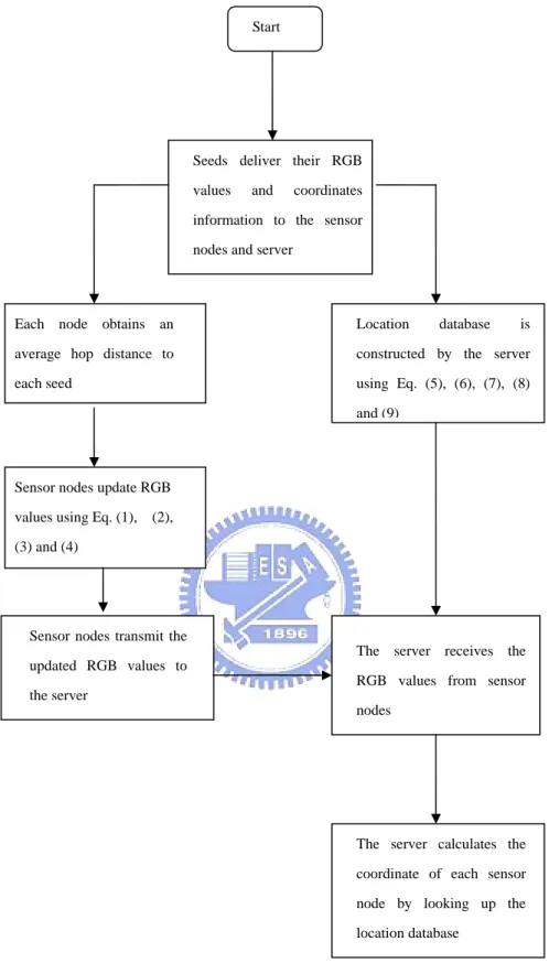
(36) 3.5 Mobility In [24] it showed mobile nodes can bridge gaps between nodes where the accurate location information cannot be obtained. In addition, It also showed that mobility is helpful for the improvement of localization accuracy. When a mobile node arrives at a new location, it sends a seed information request to other neighbors. If the neighbors have the seeds’ RGB values, they transmit packets that include the RGB values of seeds and the hop counts to seeds to the node. After receiving the packets from neighbors, the node i compares and calculates the Dik to kth seed and get the smallest Dik . With the RGB values and Dik to all seeds, the node i can calculate its RGB values using equation (1), (2), (3), and (4). The RGB values are then transmitted to the server and the position of node i will be calculated by looking up the location database. Fig. 3 is the flowchart of the CDL algorithm.. 17.

(37) Start. Seeds deliver their RGB values. and. coordinates. information to the sensor nodes and server. Each node obtains an. Location. database. is. average hop distance to. constructed by the server. each seed. using Eq. (5), (6), (7), (8) and (9). Sensor nodes update RGB values using Eq. (1),. (2),. (3) and (4). Sensor nodes transmit the The server receives the updated RGB values to RGB values from sensor the server nodes. The server calculates the coordinate of each sensor node by looking up the location database. Fig. 3. The CDL algorithm.. 18.

(38) Chapter 4 Simulation Results and Discussion To evaluate our method, the location accuracy is the main issue to be investigated. Location accuracy can be improved by several ways, including increasing the number of seeds and density of nodes or seeds. However, the tradeoff of cost and location accuracy needs to be considered carefully. In this section, we evaluate the proposed approach CDL by measuring its estimated location errors with various parameters and compared with an existing method MCL [17]. The simulation was conducted using Matlab, which is a tool for numerical computations and is powerful for its computing with matrices and vectors, and is easy for representing numerical data in graphs.. 4.1 Simulation Model Our simulation models a network where all sensor nodes are placed randomly in a 500 m × 500 m area [17]. We first introduce the random waypoint models [25], which is a popular mobility model for mobile sensor networks. In this model, a node selects its destination and velocity randomly. After it reaches the destination, it pauses for a period of time (pause time) selected randomly. In [19], the random way point model was shown to fail to provide a steady state because of the decreasing of the average node speed over time. [20] provided a proof for the phenomenon mentioned above and came up with a methodology which guarantees the constancy of the average node speed distribution. For comprising with MCL[17], we adopted the 19.

(39) modified random waypoint model from [17], in which nodes randomly choose their speed during each movement instead of selecting a certain speed for each destination. In addition, we assume the radio range is a perfect circle [17]. The node speed is uniformly distributed within [Vmin, Vmax]. Table 2 lists the simulation parameters, which are defined as follows: ¾. Seed density ( sd ): the average number of seeds in one hop transmission range [17] .. ¾. t u ：Time slot length between location announcements [17] .. ¾. Estimate error: expressed in terms of the node transmission range R .. ¾. Node density ( nd ): the average number of sensor nodes in one hop transmission range [17] .. Table 2: Simulation parameters [17]. Parameter. Value. Area size. 500 × 500 m 2. Node speed. Randomly choose from [Vmin,Vmax]. Node transmission range (R). 50 m. Pause time. 0. Number of samples maintained (for MCL). 50. Measurement period. 50 t u. Time slot length (time unit). tu. 20.

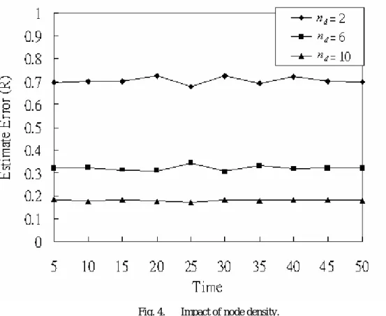
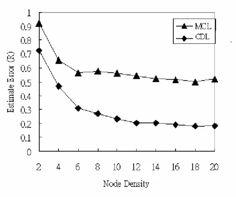
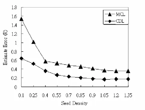
(40) Fig. 4 shows the estimate error measured in terms of the node transmission range R, for different node density ( nd ). The more the number of sensor nodes, the better the location accuracy of sensor nodes. The estimate error can be archived below 0.3 R when the node density is more than 6.. Fig. 4.. Impact of node density.. Fig. 5 shows the location estimate error in R with different number of seeds, with Vmax = R in terms of meters per time slot for nd = 10. A seed is a node aware of its location. It can assist other sensor nodes to estimate their locations. That is, with the help of information given by seeds, sensor nodes can localize their locations. With sd = 0.4, it is sufficient for CDL to perform as accurately as MCL.. 21.

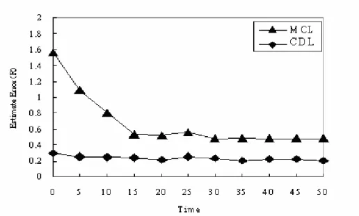
(41) Fig. 5. Impact of seed density.. 4.2 Comparison with MCL [17] We compare the CDL with MCL, which is also a range-free approach for mobile WSNs. Fig. 6 compares the localization estimate error between MCL and CDL over time with sd = 0.5, Vmin = R, and nd = 10. The MCL can exploit past information, so its accuracy improves over time. Although the CDL does not use the past information, it performs quite well and stable over time.. 22.

(42) Fig. 6. Accuracy comparison. The node density plays an important role in localization. Since the location information is provided by neighbors, the more the node density, and the more accurate the localization. Besides, the estimate error caused by the uneven distribution of nodes topology can be reduced significantly by increasing the node density. Fig. 7 shows the impact of node density on location accuracy, with Vmax = R and sd = 0.5. The accuracy of each scheme can be improved quickly by increasing the node density. However, in any case, CDL always performs better than MCL regardless of node density.. 23.

(43) Fig. 7. Impact of node density. Fig. 8 shows the accuracy of MCL and CDL improve with the increasing of seed density, with Vmax = R and nd = 10.. MCL performs localization by collecting. information from seeds or sensor nodes which is one hop away from seeds. As a result, seed density is a critical factor for MCL. The location accuracy improves significantly as the seed density soars. For CDL, its location accuracy does not rely on sufficient numbers of seed nodes, because CDL collects location information from all seeds. It performs good with few seeds, compared to MCL.. 24.

(44) Fig. 8. Impact of seed density.. 25.

(45) Chapter 5 Conclusions and Future Work 5.1 Concluding Remarks Localization is a critical issue in wireless sensor network. With the aid of locations of sensor nodes, for example, the efficiency of routing can be improved significantly. We have proposed an efficient Color-theory based Dynamic Localization (CDL) for mobile wireless sensor networks. The basic idea of CDL is based on color theory, which exploits the changes of colors with distances to localize sensor nodes. CDL is suitable in the scenarios that need a centralized server to collect and monitor all users, such as in health-care systems and hospital monitor systems. Our simulation results reveal the location estimate error can be reduced up to 0.2 R when the seed density = 0.8 and node density = 0.5. In addition, the location accuracy of CDL is 40% - 50% better than that of MCL [17]. 5.2 Future Work To enhance location accuracy, the uniqueness of mapping RGB values to coordinates for building up the location database can be studied for developing a better mapping algorithm. In addition, we will implement the CDL in real mobile wireless sensor networks, such as a Berkeley Mote platform, to further evaluate its localization effectiveness.. 26.

(46) Bibliography [1] R. K. Patro, “Localization in wireless sensor network with mobile beacons,” in Proc. 23rd IEEE Convention on Electrical and Electronics Engineers, pp. 22 24 , Sept. 2004.. [2] F. Mondinelli and Z. M. Kovacs-Vajna, “Self-localizing sensor network architectures,” in IEEE Transactions Instrumentation and Measurement vol. 53, pp. 277 – 283, Apr. 2004.. [3] Y. Shang, J. Meng and H. Shi,“A new algorithm for relative localization in wireless sensor networks,” in Proc Parallel and Distributed Processing Symposium , pp.24 , Apr. 2004.. [4] W. Su,S.J. Lee and M. G, ”Mobility prediction in wireless networks,” in Proc MILCOM 2000. vol. 1, pp. 491 – 495, Oct. 2000.. [5]. P. Bergamo and G. Mazzini, “Localization in sensor networks with fading and mobility,” in Proc The 13th IEEE International Symposium on Personal, Indoor and Mobile Radio Communications ,vol.2, pp.750 - 754 , Sept. 2002.. [6] G. Mainetto, “A predictive model for indoor tracking of mobile users,” in Proc.. 27.

(47) 14th International Workshop on Database and Expert Systems Applications, pp. 921 – 925, Sept. 2003.. [7] P. Bahl and V. N. Padmanabhan, “RADAR: An In-Building RF-Based User Location and Tracking System,” in Proc. IEEE INFOCOM, Mar. 2000.. [8] K. Kaemarungsi and P. Krishnamurthy , “Properties of indoor received signal strength for WLAN location fingerprinting,” in Proc. MOBIQUITOUS, pp.14 – 23, . Aug. 2004. [9] K. Kaemarungsi and P. Krishnamurthy “Modeling of indoor positioning systems based on location fingerprinting,” in Proc. IEEE INFOCOM, vol. 2, pp. 1012 – 1022, Mar. 2004.. [10] N. B. Priyantha, A. Chakraborty and H. Balakrishnan, “The cricket location-support system,” in Proc. MOBICOM 2000, pp. 32-43, Aug. 2000.. [11] D. Niculescu and B. Nath, “Ad hoc positioning system (APS),”in. IEEE. GLOBECOM, vol. 5, pp. 2926 - 2931, Nov. 2001.. [12] N. Bulusu , J. Heidemann and D. Estrin, “GPS-less low-cost outdoor localization for very small devices,” in IEEE Personal Communications, vol. 7, pp. 28 – 34, Oct. 2000.. [13] T. Kitasuka , T. Nakanishi and A. Fukuda, “ Location estimation system using wireless ad-hoc networks,” in Wireless Personal Multimedia Communications, vol.. 28.

(48) 1, pp. 305 – 309, Oct. 2002.. [14] M. L. Sichitiu and V. Ramadurai,“Localization of wireless sensor networks with a mobile beacon,” in IEEE Mobile Ad-hoc and Sensor Systems International Conference, pp. 174 - 183, Oct. 2004.. [15] G. L. Suu and W. Guo, “Comparison of distributed localization algorithms for sensor network with a mobile beacon,” in IEEE Networking, Sensing and Control International Conference, vol. 1, pp. 536 - 540 , Mar. 2004.. [16] B. Milic, N. Milanovic and M. Malek, ”Prediction of partitioning in location-aware mobile ad hoc networks,” in Proc. 38th Annual Hawaii International Conference , pp. 306 – 306, Jan. 2005.. [17] L. Hu and D. Evans, “Localization: localization for mobile sensor networks,” in Proc.10th annual international conference on Mobile computing and networking, pp. 45-57, Sept. 2004.. [18] P. Zelanski and M. P. Fisher, “The Camara” [Online] Available: http://www.cse.fau.edu/~maria/COURSES/COP4930-GS/color2notes.htm.. [19] J. Yoon, M. Liu and B. Noble,“Random waypoint considered harmful,” in Proc. IEEE INFOCOM, vol. 2, pp. 1312 – 1321, Apr. 2003.. [20] G. Lin, G. Noubir and R. Rajaraman, “Mobility models for ad hoc network simulation,” in Proc. IEEE INFOCOM, vol. 2 Mar. 2004, pp. 1312 – 1321.. 29.

(49) [21] DevX.com, “Color Models” [Online] Available: http://www.devx.com/projectcool/Article/19954/0/page/7.. [22] Wikipedia, “HSV color space” [Online] Available: http://www.answers.com/topic/hsv-color-space.. [23] E. Vishnevsky, “RGB to HSV & HSV to RGB” [Online] Available:. http:// www.cs.rit.edu/~ncs/color/t_convert.html.. [24] J. G. Lim and SV Rao, “Mobility-enhanced positioning in ad hoc networks”, in Wireless Communications and Networking, Mar. 2003.. [25] D. B. Johnson and D. A. Maltz, “Dynamic source routing in ad hoc wireless networks,” in Mobile Computing, Imielinski and Korth, Eds. Kluwer Academic Publishers, 1996.. [26] Y. Shang, W. Ruml, Y. Zhang, and M. Fromherz, “Localization from mere connectivity”, in Proc ACM MobiHoc, June 2003, pp. 201–212.. 30.

(50)