沉浸有限元素法於彈性界面與流構耦合問題的計算與誤差估計

(1)

行政院國家科學委員會專題研究計畫成果報告

沉浸有限元素法於彈性界面與流構耦合問題的計算與誤差

估計

研究成果報告(精簡版)

計畫類別：個別型

計畫編號： NSC 99-2115-M-009-001-

執行期間： 99 年 08 月 01 日至 100 年 07 月 31 日

執行單位：國立交通大學應用數學系（所）

計畫主持人：吳金典

計畫參與人員：碩士班研究生-兼任助理人員：蔣明虔

碩士班研究生-兼任助理人員：楊濟俊

報告附件：出席國際會議研究心得報告及發表論文

處理方式：本計畫涉及專利或其他智慧財產權，2 年後可公開查詢

中華民國 100 年 10 月 29 日

(2)

Elsevier Editorial System(tm) for Journal of Computational and Applied Mathematics Manuscript Draft

Manuscript Number: CAM-D-11-00770

Title: Numerical studies on structure-preserving algorithms for surface acoustic wave simulations Article Type: Research Paper

Section/Category: 65Fxx

Keywords: Palindromic, structure-preserving, surface acoustic wave, finite element Corresponding Author: Dr. Chin-Tien Wu,

Corresponding Author's Institution: Mathematical Modelling and Scientific Computation First Author: Tsung-Ming Huang

(3)

Numerical Studies on Structure-Preserving Algorithms for

Surface Acoustic Wave Simulations

1

Tsung-Ming Huanga, Chin-Tien Wub,∗, Tiexiang Lic

a_{Department of Mathematics, National Taiwan Normal University, Taipei 116, Taiwan. E-mail:}

[email protected].

b_{Department of Applied Mathematics, National Chiao Tung University, Hsinchu 300, Taiwan. E-mail:}

c_{Department of Mathematics, Southeast University, Nanjing 211189, Peoples Republic of China.}

E-mail: [email protected].

Abstract

We study the generalized eigenvalue problems (GEPs) derived from modeling the surface acoustic wave in piezoelectric materials with periodic inhomogenuity. The eigenvalues appear in the reciprocal pairs due to periodic boundary conditions in the modeling. By transforming the GEP into a T-palindromic quadratic eigenvalue problem (TPQEP), the reciprocal relationship of the eigenvalues can be maintained. In this paper, we outline four recently developed structure-preserving algorithms, SA, SDA, TSHIRA and GTSHIRA, for solving the TPQEP. Numerical comparisons on the accuracy and the computational costs of these algorithm are presented. The eigenvalues close to unit circle on the complex plane are of interests in the area of filter and sensor designs. Our numerical results show that the Arnoldi-type structure-preserving algorithms TSHIRA and GTSHIRA with ”re-sympletic” and ”re-bi-isotropic”, respectively, are as accurate as the SA and SDA algorithm, and more efficient in finding these eigenvalues.

1. Introduction

In this paper we consider the generalized eigenvalue problem (GEP) of the form [ M1 G F⊤ 0 ] [ ψi ψℓ ] + λ [ 0 F G⊤ M2 ] [ ψi ψℓ ] = 0, (1)

where M₁⊤ = M1 ∈ Cn×n, M2⊤ = M2 ∈ Cm×m, F and G ∈ Cn×m with m ≪ n, and

the supscript “⊤” denotes the complex transpose. If M1 and M2 are nonsingular, then

(1) can be reduced as the T-palindromic quadratic eigenvalue problem (TPQEP) of the form

P(λ)x ≡ (λ2_A⊤

1 + λA0+ A1)x = 0, (2)

∗_{Corresponding author: Chin-Tien, Wu, Tel: +886-3-5712121-ext-56424.} Manuscript

(4)

where x = ψℓ, ψi=−M1−1(λF + G)ψℓ, A1 = F⊤M1−1G, A0= F⊤M1−1F + G⊤M1−1G− M2; (3) or x = ψi, ψℓ=−λ−1M2−1(F⊤+ λG⊤)ψi, A1 = GM2−1F⊤, A0= F M2−1F⊤+ GM2−1G⊤− M1. (4)

By taking the transpose ofP(λ) in (2) and multiplying it by 1/λ2 _{it is easily seen that}

the eigenvalues of P(λ) appear in the reciprocal pairs (λ, 1/λ) (including 0 and ∞). Since the nullity of A1 = GM2−1F⊤ in (4) is larger or equal to n− m, P(λ) in (2)

with A0 and A1deﬁned in (4) has n− m trivial zero and inﬁnite eigenvalues which are

not interested. We are only interested in ﬁnding 2m(≪ 2n) nontrivial eigenpairs of P(λ). The GEP (1) can be solved by traditional methods such as QZ and Arnoldi method. But it does not guarantee that half of the computed eigenvalues lie inside of the unit circle and the others are outside [9]. For solving TPQEP (2) with small and dense matrices A0

and A1, some pioneering works [7, 13, 14] have been done for preserving the reciprocity

of the eigenvalues basing on a good linearization of (2) which transforms (2) into the form λZ⊤+ Z. Some structure-preserving methods [7, 18, 19] were proposed for solving (λZ⊤+ Z)u = 0. A structure-preserving doubling algorithm for solving (2) was devel-oped in [5] via the computation of a solvent of a nonlinear matrix equation associated with (2). Another structure-preserving algorithm based on (S + S−1)-transform [12] and Patel’s approach [17] was developed in [8]. For problems with large and sparse matrices

A0 and A1, a structure-preserving algorithm using (S + S−1)-transform and

implicity-restarted shift-and-invert Arnoldi method was also developed for searching eigenvalues in a speciﬁed region of interests [8].

The GEP (1) typically arises in many application areas including rail vibrations of fast train, surface acoustic wave (SAW) in filter design and crack modeling, etc [6]. In these areas, an accurate and efficient eigensolver which preserves the reciprocal relation-ship of the associated eigenpairs is needed. In this paper, we would like to compare the accuracy and computational costs of the above mentioned algorithms for computing reciprocal eigenpairs in a SAW device [22]. The SAW filter plays an important role in telecommunication filters [4, 16] and sensor technologies [2] etc. These filters are built on the physical property of piezoelectric materials, that electrical charges induce mechanical deformations and vice versa. The main component (or cell) of a SAW filter composes of a piezoelectric substrate and the input and output interdigital transducers (IDT). An input electrical signal from the input IDT produces a surface acoustic wave, traveling through periodically arranged electrodes and the output IDT picks up the output elec-trical signal. Depending on the material properties of the piezoelectric substrate (PZT) and the metallic electrode, and the gap length between the electrodes, frequencies in a desired range can be stopped or filtered out. In the filter design, it is important to know the stop band width and the center frequency fc of the filter where fc= v_λs

(5)

stop band width can be determined by experiments or computation. In computational approach, the dispersion diagram needs to be generated in which a GEP of the form (1) associated with each frequency in the search range has to be solved [9].

This paper is organized as follows. We shall first introduce finite element modelling for a simple SAW resonator in Section 2. For more finite element simulations of piezoelectric devices in two dimension (2D) and three dimension (3D), one can refer to the works done by Allik, Koshiba, Lerch, Buchner and Mohamed etc.,[1, 3, 10, 11]. In Section 3, we introduce four structure-preserving algorithms developed in [5, 8] to solve the TPQEP (2) and the GEP (1) resulted from our FEM model. Our numerical experiments in Section 4 compare the efficiency and accuracy of the structure-preserving algorithms for solving the GEP (1). Finally, we conclude the paper in Section 5.

2. Surface wave propagation

To model the wave propagation in a SAW device, we assume that a large number of electrodes are placed equally-spaced along a straight line on the PZT substrate. Accord-ing to the Floquet-Bloch theory, one can reduce the problem to a sAccord-ingle cell domain with one electrode by assuming the wave ψ is quasi-periodic of the form

ψ(x1, x2) = ψp(x1, x2)e(α+ıβ)x1, ψp(x1+ p, x2) = ψp(x1, x2),

where x1 is the wave propagation direction, p is the length of the unit cell (i.e. the

periodic interval), α and β are the attenuation and phase shift along the wave propagation direction, respectively.

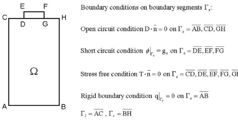
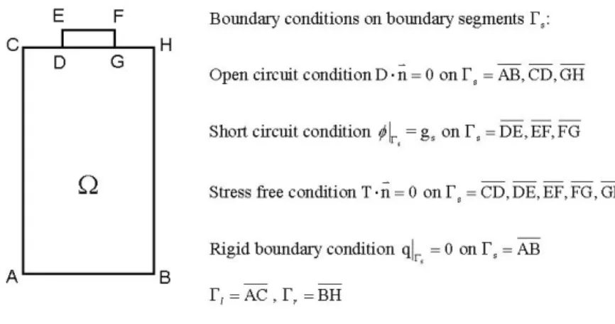
Let Ω denote the piezoelectric substrate with a single IDT as shown in Figure 1, and Γℓand Γrdenote the left and right boundary segments of Ω, respectively. For the general

anisotropic PZT substrates, under the assumption of linear piezoelectric coupling, the elastic and electric ﬁelds interact following the general material constitution law below

T = cES− e⊤E,

D = eS + εSE, (5)

where vectors T , S, D and E are the mechanical stress, strain, dielectric displacement and the electric ﬁeld, respectively, and the matrices cE_{, ε}S _{and e are the elasticity constant,}

dielectric constant and piezoelectric constant matrices measured at constant electric and constant strain ﬁelds at constant temperature. By applying the virtual work principle to the equation (5), the equilibrium state satisﬁes the following equation:

∫ Ω (δS)⊤[cES + e⊤(∇ϕ)]dV + ∫ Ω (∇δϕ)⊤[eS− εS(∇ϕ)] dV + ∫ Ω (δu)⊤ρ¨u dV = ∫ Γl∪Γr [ (δu)⊤(T· ⃗n) + (δϕ)⊤(D· ⃗n)] dA, (6) where ρ is the mass density, u = [u1, u2, u3]⊤ is the displacement vector, ϕ is the electric

potential that satisﬁes∇ϕ = E, S = [∂u1

∂x, ∂u2 ∂y , ∂u3 ∂z , ∂u2 ∂z + ∂u3 ∂y , ∂u3 ∂x + ∂u1 ∂z, ∂u1 ∂y + ∂u2 ∂x]⊤,

(6)

Figure 1: A 2D single cell domain of a LSAW resonator and boundary conditions

the notation ψ = [u⊤, ϕ]⊤ and the subscript i, ℓ and r refer to nodal point index in the interior, the left boundary and the right boundary of the domain Ω, respectively. Using the periodic boundary conditions, proposed by Buchner [3],

Tr· nr=−γTℓ· nℓ, Dr· nr=−γDℓ· nℓ with γ = e−(α+ıβ),

the ﬁnite element discretization to (6) on the domain Ω [9] can be written in the following matrix form

C(ω)ψ≡ [K − ω2M + ıω(κ1K + κ2M )]ψ = 0, (7)

where κ1, κ2> 0 are the viscous damping and mass damping respectively. By ordering

the nodal unknown ψ according the order of subscripts ℓ, i and r, the matrices K and

M , and the vector ψ can be partitioned as following:

K =   Kℓℓ K ⊤ iℓ 0 Kiℓ Kii Kir 0 K_ir⊤ Krr   , M =   Mℓℓ M ⊤ iℓ 0 Miℓ Mii Mir 0 M_ir⊤ Mrr   ,

where Kii, Mii ∈ Rn×n, Kℓℓ, Krr, Mℓℓ, Mrr ∈ Rm×m, Kiℓ, Kir, Miℓ, Mir ∈ Rn×m, and ψ = [ψ_ℓ⊤, ψ_i⊤, ψ_r⊤]⊤ with ψi ∈ Cn, ψℓ, ψr∈ Cm (m≪ n). Obviously the matrix C(ω) in

(7) can also be partitioned into

C(ω)≡ C ≡   Cℓℓ C ⊤ iℓ 0 Ciℓ Cii Cir  

(7)

By setting ψr= λψℓ, the equation (7) leads to the generalized eigenvalue problem ([ Cii Ciℓ C_ir⊤ 0 ] − λ [ 0 Cir C_iℓ⊤ Cbb ]) [ ψi ψℓ ] = 0, (8) where Cbb:= Cℓℓ+ Crr.

Since the viscosity is small for PZT substrates and metals in SAW devices, the at-tenuation factor α of surface waves is close to zero. As a result, the propagation factor

λ are generally near the unit circle thereafter denoted byU. Furthermore, for frequency ω in the stopping band, the frequency shift parameter β shall be close to π when the

periodic interval p (i.e. the domain width here) equals to half of the incident wave length

λs. Therefore, we are interesting in ﬁnding λ close to U, especially for those are near −1 on the complex plane. Notice that eigenvalues of (2) appear in the reciprocal pairs

(λ, 1/λ). In the following sections, we aim to discuss the eﬃciency and accuracy of the structure-preserving algorithms [5, 8] for solving the eigen-curves λ(ω) and the associated eigenvectors of (8).

3. Structure-preserving Algorithms

In this section, we shall introduce four structure-preserving algorithms developed in [5, 8] to solve the TPQEP (2) and discuss the computation costs of these algorithms in solving the GEP (1). In the following, we suppose m reciprocal pairs of eigenvalues near U are desired.

3.1. structure-preserving doubling algorithm

For solving the TPQEP (2) with A0, A1∈ Cm×mdeﬁned in (3), a structure-preserving

doubling algorithm (SDA) was developed in [5] via the computation of a solvent of a nonlinear matrix equation associated with (2). That isP(λ) can be factorized as

P(λ) = (λA⊤

1 − X)X−1(λX− A1) (9)

for some nonsingular X with X⊤ = X if and only if X satisﬁes the following nonlinear matrix equation (NME):

A⊤₁X−1A1+ X + A0= 0.

Combining SDA in [5], the GEP (1) can be solved by Algorithm 1. The advantages of Algorithm 1 are as following: (i) the computed eigenvalues are guaranteed to appear in reciprocal pair since the eigenvalues of the matrix pencils λA⊤₁ − X and λX − A1, which

are reciprocal pairs, are the eigenvalues ofP(λ) in (9) and (ii) the convergence rate of the SDA is proved to be quadratic [5] if there are no eigenvalues ofP(λ) located on unit circle.

Next, let’s discuss the computational costs of Algorithm 1. To mimic the computation cost in the LU factorization of the matrix M1obtained from ﬁnite element discretization,

we reorder the nodal indices so that the matrix M1 has narrower band structure. Let

(8)

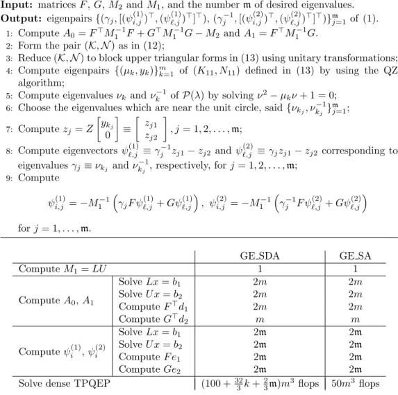
Algorithm 1 GE SDA

Input: matrices F , G, M2and M1, tolerance η and the number m of desired eigenvalues.

Output: eigenpairs{(γj, [(ψ (1) i,j)⊤, (ψ (1) ℓ,j)⊤]⊤), (γj−1, [(ψ (2) i,j)⊤, (ψ (2) ℓ,j)⊤]⊤)} m j=1of (1). 1: Compute A0= F⊤M1−1F + G⊤M1−1G− M2 and A1= F⊤M1−1G.

2: Set k = 0, Yk = A1, Xk=−A0 and Zk= 0.

3: repeat

4: Compute Yk+1= Yk(Xk− Zk)−1Yk, Xk+1= Xk− Yk⊤(Xk− Zk)−1Yk, and Zk+1= Zk+ Yk(Xk− Zk)−1Yk⊤;

5: Set k = k + 1;

6: until∥Xk− Xk−1∥ ≤ η∥Xk∥

7: Compute the left and right eigenpairs{(λj, ψ

(1) ℓ,j), (λj, ψ (r) ℓ,j)} m j=1of Xkψℓ= λA⊤1ψℓ;

8: Choose the eigenpairs which associated eigenvalues are near the unit circle, said

{(λj, ψ (1) ℓ,j), (λj, ψ (r) ℓ,j)} m j=1; 9: Solve (λjXk− A1)ψ (2) ℓ,j = Xkψ (r)

ℓ,j and set γj= λ−1j for j = 1, . . . , m;

10: Compute ψ(1)_i,j =−M₁−1 ( γjF ψ (1) ℓ,j + Gψ (1) ℓ,j ) , ψ(2)_i,j =−M₁−1 ( γ_j−1F ψ_ℓ,j(2)+ Gψ(2)_ℓ,j ) for j = 1, . . . , m.

Algorithm 1 requires solving eF ≡ U−1L−1F and eG≡ U−1L−1G, and matrix

multipli-cations of F⊤F , Ge ⊤G and Fe ⊤G. In Steps 3.1-3.1, one LU factorization (2me 3_{/3 ﬂops),}

two forward and back substitutions (4m3flops) and three matrices multiplications (6m3 flops) are required for each iterate k. Next, computing the left and right eigenpairs in Step 3.1 and solving ψ_ℓ,j(2) in Step 3.1 take 100m3 flops and 2mm3/3 flops, respectively.

Finally, it also requires 2m forward and back substitutions to compute{ψ(1)i,j, ψ

(2)

i,j}mj=1in

Step 3.1. The total cost of Algorithm is summarized in Table 1.

3.2. structure-preserving algorithm

Another structure-preserving algorithm (SA) developed in [8] is based on the (S +

S−1_{)-transform [12] and Patel’s approach [17] for solving the TPQEP (2) with A}

0, A1∈

Cm×m _{deﬁned in (3). The idea is, ﬁrst, to linearize the TPQEP as the following special}

GEP: (M − λL) [ x y ] = 0, (10)

where λy = A1x, and

M = [ A1 0 −A0 −I ] , L = [ 0 I A⊤₁ 0 ] . (11)

Obviously, the matrix pencilM − λL is ⊤-symplectic, i.e., it satisﬁes MJ M⊤=LJ L⊤

J =

[

0 Im

]

(9)

pairs (λ, 1/λ). Secondly, the (S + S−1)-transform is applied onM − λL and the pencil is now transformed into a ⊤-skew-Hamiltonian pencil K − µN , i.e., (KJ )⊤ = −KJ , (N J )⊤=−N J : K − µN ≡ [(LJ M⊤+MJ L⊤)− µLJ L⊤]J⊤ = [ A0 A⊤1 − A1 A1− A⊤1 A0 ] − µ [ −A1 0 0 −A⊤₁ ] . (12)

The two eigenvalues λ and µ are then related by the relationship µ = λ + 1/λ. The relationship between eigenpairs of the TPQEP in (2) and the⊤-skew-Hamiltonian pair (K, N ) in (12) is stated in the following theorem.

Theorem 3.1. [8] Let (K, N ) be defined in (12). If zs= [z1⊤, z2⊤]⊤ with z1, z2∈ Cm is

an eigenvector of (K, N ) corresponding to eigenvalue µ and ν satisfies ν + 1

ν = µ, then

1

νz1−z2and νz1−z2are eigenvectors of the TPQEP in (2) corresponding to eigenvalues ν and 1

ν, respectively.

Finally, based on Patel’s approach [17], the matrix pair (K, N ) can further be reduced to a block triangular structure as following

K := Q⊤_{KZ =} [ K11 K12 0 K₁₁⊤ ] , N := Q⊤N Z = [ N11 N12 0 N₁₁⊤ ] , (13)

where K11∈ Cm×mis upper Hessenberg, N11∈ Cm×mis upper triangular, and Q, Z are

unitary satisfying

Q =J⊤ZJ .

We then apply the QZ algorithm to (K11, N11) for computing the m eigenpairs{(µk, yk)}mk=1.

Consequently,{(µk, Z [ yk 0 ] )}m

k=1 are the m eigenpairs of (K, N ). Combining the above

procedures and the structure-preserving algorithm in [8], the GEP (1) can be solved by Algorithm 2.

The computational costs in Steps 3.2 and 3.2 of Algorithm 2 are the same that in Steps 3.1 and 3.1 of Algorithm 1. The SA processes in Steps 3.2-3.2 of Algorithm 2 require approximately 50m3_{ﬂops [8] to compute the eigenpairs of the TPQEP (2) with}

small size matrices A0 and A1 in (3). The comparison of the computation costs for

GE SDA and GE SA is listed in Table 1.

3.3. ⊤-skew-Hamiltonian implicit-restarted Arnoldi algorithm

In the above mentioned GE SDA and GE SA algorithms, the GEP (1) is transformed into the TPQEP (2) through equations in (3) where M₁−1F and M₁−1G are solved by

LU factorization on the matrix M1. The computation costs in this step increase in the

amount of 2m times n2_{. Since the GE SDA and GE SA algorithms are then working on}

(10)

Algorithm 2 GE SA

Input: matrices F , G, M2and M1, and the number m of desired eigenvalues.

Output: eigenpairs{(γj, [(ψ (1) i,j)⊤, (ψ (1) ℓ,j)⊤]⊤), (γj−1, [(ψ (2) i,j)⊤, (ψ (2) ℓ,j)⊤]⊤)} m j=1of (1). 1: Compute A0= F⊤M1−1F + G⊤M1−1G− M2 and A1= F⊤M1−1G.

2: Form the pair (K, N ) as in (12);

3: Reduce (K, N ) to block upper triangular forms in (13) using unitary transformations;

4: Compute eigenpairs {(µk, yk)}mk=1 of (K11, N11) deﬁned in (13) by using the QZ

algorithm;

5: Compute eigenvalues νk and νk−1 ofP(λ) by solving ν

2_{− µ}

kν + 1 = 0;

6: Choose the eigenvalues which are near the unit circle, said{νkj, ν

−1 kj } m j=1; 7: Compute zj= Z [ ykj 0 ] ≡ [ zj1 zj2 ] , j = 1, 2, . . . , m;

8: Compute eigenvectors ψ(1)_ℓ,j ≡ γ_j−1zj1− zj2and ψ

(2) ℓ,j ≡ γjzj1− zj2 corresponding to eigenvalues γj≡ νkj and ν −1 kj , respectively, for j = 1, 2, . . . , m; 9: Compute ψ(1)_i,j =−M₁−1 ( γjF ψ (1) ℓ,j + Gψ (1) ℓ,j ) , ψ(2)_i,j =−M₁−1 ( γ_j−1F ψ_ℓ,j(2)+ Gψ(2)_ℓ,j ) for j = 1, . . . , m. GE SDA GE SA Compute M1= LU 1 1 Compute A0, A1 Solve Lx = b1 2m 2m Solve U x = b2 2m 2m Compute F⊤d1 2m 2m Compute G⊤d2 m m Compute ψ_i(1), ψ(2)_i Solve Lx = b1 2m 2m Solve U x = b2 2m 2m Compute F e1 2m 2m Compute Ge2 2m 2m

Solve dense TPQEP (100 + 32 3k +

2 3m)m

3_ﬂops _50m3 _ﬂops

Table 1: The computational costs of GE SDA and GE SA where k denotes the total iterations to obtain convergent Xkin Lines 3.1-3.1 of GE SDA.

the TPQEP is relatively small.

In the following, we introduce two Arnoldi-type algorithms in which the GEP (1) is transformed into the TPQEP (2) through equations in (4). Since the matrix size m of

M2 is much smaller, the cost in solving M2−1F⊤ and M2−1G⊤ by LU factorization of

M2 can now be ignored. Following the same idea in Section 3.2, the TPQEP (2) with

(11)

the equations (10) and (12) withJ = [

0 In −In 0

]

. Instead of taking Patel’s approach, we seek the eigenvalues of the matrix pair (K, N ) by some implicit-restart Arnoldi algo-rithms. Although the Arnoldi algorithm is working on the matrices with size 2n× 2n now, saving on computation costs is expected when fast convergence of the Arnoldi iter-ations can be achieved. In the following, we sketch the key steps and theorems that are employed in developing Arnoldi algorithm.

Let τ be a shift value and τ /∈ σ(M, L) where σ(A, B) denotes the set of all eigenvalues of any matrix pair (A, B). Then, we have µ0≡ τ +τ−1∈ σ(K, N ). Deﬁne the shift-invert/

transformation bK − bµ bN for K − µN with bµ = _µ_−µ1

0 and b K ≡ −τN = τ [ A⊤₁ 0 0 A1 ] , (14a) b N ≡ −τ(K − µ0N ) = (M − τL) J ( M⊤_{− τL}⊤)_J⊤_, _(14b)

where bK and bN are ⊤-skew-Hamiltonian. Furthermore, from the deﬁnition of bN in (14b), b

N can be factorized as bN = N1N2, where

N1=M − τL, N2=J (M⊤− τL⊤)J⊤ (15)

are nonsingular and satisfyN₂⊤J = J N1. The GEP bKz = bµ bN z is then equivalent to the

eigenvalue problemB˜z = bµ˜z, where

B ≡ N−1

1 KNb 2−1 (16)

is⊤-skew-Hamiltonian, i.e., J B⊤=BJ , and ˜z = N2z. Now, according to the followingˆ

two main theorems proved in [8, 15], the⊤-skew-Hamiltonian implicity-restarted Arnoldi (TSHIRA) algorithm as shown in Algorithm 4 can be employed to solve this eigenvalue problem.

Let’s deﬁne the Krylov matrix with respect to u1by

Kj≡ Kj[B, u1] = [u1,Bu1, . . . , Bj−1u1], 1≤ j ≤ n.

The two main theorems in [8, 15] are as follows:

Theorem 3.2. [15] Let B ∈ C2n×2n _be _{⊤-skew-Hamiltonian and K}

j be a Krylov ma-trix with rank(Kj) = j. Then span(Kj) is ⊤-isotropic and if Kj = UjRj is a QR-factorization, then

BUj = UjHj+ ˜uj+1e⊤j,

where Hj ∈ Cj×j is unreduced upper Hessenberg, Uj ∈ C2n×j is orthonormal and ⊤-isotropic, and ˜uj+1∈ C2n is a suitable vector such that

(12)

Theorem 3.3. [8, 15] LetB ∈ C2n×2n _be _{⊤-skew-Hamiltonian. If rank(K}

n) = n, then there is a unitary⊤-symplectic matrix U with Ue1= u1 such that

UH_{BU =} [ Hn Sn 0 H_n⊤ ] ,

where Hn≡ [hij] is unreduced upper Hessenberg and Sn is⊤-skew-symmetric.

Based on Theorem 3.2, the jth step of TSHIRA is given by

hj+1,juj+1=Buj− j

∑

i=1

hijui, (17)

where hij = uHi Buj, i = 1, . . . , j and hj+1,j > 0 is chosen so that ∥uj+1∥2 = 1. In

order to guarantee the⊤-isotropic property of the space span{u1, . . . , uj+1} is preserved

within machine precision, reorthogonalizing uj+1 againstJ Uj is necessary. As a result,

the equation (17) is modiﬁed into

hj+1,juj+1=Buj− j ∑ i=1 hijui− j ∑ i=1 tijJ ¯ui,

where tij =−u⊤i J Buj, i = 1, . . . , j. The above procedure is stated in Algorithm 3.

Finally, we present TSHIRA with Krylov-Schur restart to solve the eigenvalue prob-lemB˜z = bµ˜z in Algorithm 4. Once the eigenpair (ˆµ, ˜z) is obtained, one can recover the eigenpair (µ, z) of (K, N ) from the relationship ˆu = _µ_−µ1

0 and the solution of the linear

systemN2z = ˜z. The reciprocal eigenpair (λ,_λ1) and the associated eigenvectors of the

TPQEP (2) are then followed from Theorem 3.1.

Algorithm 3 The jth⊤-isotropic Arnoldi step

Input: ⊤-skew-Hamiltonian B and Uj= [u1,· · · , uj] with UjHUj= Ij and Uj⊤J Uj= 0.

Output: [h1,j,· · · , hj+1,j] and uj+1. 1: Compute uj+1=Buj; 2: for i = 1, . . . , j do 3: hij = uHi uj+1, uj+1= uj+1− hijui 4: end for 5: for i = 1, . . . , j do 6: tij = u⊤i J⊤uj+1, uj+1= uj+1− tijJ ¯ui 7: end for

8: Set hj+1,j :=∥uj+1∥2and uj+1:= uj+1/hj+1,j.

3.4. Generalized⊤-skew-Hamiltonian implicity-restarted Arnoldi algorithm

(13)

Algorithm 4 [8] TSHIRA for solvingB˜z = bµ˜z

Input: ⊤-skew-Hamiltonian matrix B with starting vector u1.

Output: eigenpairs (bµi, ˜zi), i = 1, . . . , m ofB.

1: Use Algorithm 3 with starting vector u1 to generate the mth step of ⊤-isotropic

Arnoldi decomposition:

BUm= UmHm+ hm+1,mum+1e⊤m;

2: repeat

3: Use Algorithm 3 to extend the mth step of ⊤-isotropic Arnoldi decomposition to the (m + p)th step of⊤-isotropic Arnoldi factorization:

BUm+p= Um+pHm+p+ hm+p+1,m+pum+p+1e⊤m+p.

4: Use Krylov-Schur restarting scheme [20, 21] to reform a new⊤-isotropic Arnoldi decomposition with order m.

5: until wanted m eigenpairs ofB are convergent

This may result in losing some accuracy of the eigevector z. In order to eliminate this ex-tra computational cost and to prevent the inaccuracy, a generalized⊤-skew-Hamiltonian implicity-restarted Arnoldi (GTSHIRA) algorithm is proposed in [8]. The idea is to solve the GEP bKz = bµ bN z in (14) directly through bi-reorthogonalization and bi-⊤-isotropic processes. The GTSHIRA algorithm is based on following two theorems.

Theorem 3.4. [8] Let B ≡ N₁−1KNb ₂−1 with bN = N1N2 be ⊤-skew-Hamiltonian. Let

Kj ≡ Kj[B, u1] be the Krylov matrix with rank(Kj) = j. If N−1

2 Kj= ZjR2,j and N1Kj = YjR1,j

are QR-factorizations, where Zj, Yj ∈ C2n×j are orthonormal and R2,j, R1,j are

nonsin-gular upper triannonsin-gular, then we have

b

KZj = YjHbj+byj+1e⊤j (18) and

b

N Zj = YjRbj, (19)

where bHj ∈ Cj×j is unreduced upper Hessenberg, bRj ∈ Cj×j is nonsingular upper trian-gular, and Yj and Zj are ⊤-bi-isotropic such that

Y_jHbyj+1= 0 and Zj⊤J byj+1= 0, for a suitablebyj+1∈ C2n.

Theorem 3.5. [8] Let B = N₁−1KNb ₂−1 with bN = N1N2 be ⊤-skew-Hamiltonian and

(14)

matrices U and V satisfying V = J⊤UJ , Ue1 = u1 and Ve1 = N1u1/∥N1u1∥2 such that V⊤_{KU =}_b [ b Hn Sbn 0 Hb_n⊤ ] , V⊤N U =b [ b Rn Tbn 0 Rb⊤_n ] ,

where bHnis unreduced upper Hessenberg, bRn is nonsingular upper triangular and bSn, bTn are⊤-skew-symmetric.

Based on Theorems 3.4 and assuming that the ﬁrst (j−1)th step in GTSHIRA follows the generalized⊤-isotropic Arnoldi process, i.e.,

b

N Zj₋₁= Yj₋₁Rbj₋₁, (20)

by comparing the jth columns of both sides in (19) at the jth step, one has b N zj= j₋₁ ∑ i=1 brijyi+brjjyj. (21)

With (20), (21) can be rewritten as br−1 jj zj= bN−1yj− j−1 ∑ i=1 erijzi, (22) where [er1j, . . . ,erj_−1,j]⊤ :=−br−1jj Rb−1j₋₁[br1j, . . . ,brj_−1,j]⊤,

andbrjj in (22) is chosen so that ∥zj∥2= 1. Since ZjHZj = Ij, the coeﬃcienterij in (22)

can be evaluated by

erij = zjHNb−1yj, i = 1, . . . , j− 1.

Finally, from (18), the vector yj+1in the jth step of the generalized⊤-isotropic Arnoldi

process is given by bhj+1,jyj+1= bKzj− j ∑ i=1 bhijyi, where bhij = yiHKzb j,

and bhj+1,j > 0 is chosen so that∥yj+1∥2= 1.

Notice that, in theory, zjand yj+1are orthogonal toJ ¯YjandJ ¯Zj, respectively, in

ex-act arithmetic. However, in prex-actice, roundoﬀ errors may cause y_i⊤J⊤zj and z⊤i J⊤yj+1, i = 1, . . . , j, to be some nonzero tiny values. Therefore, in order to preserve the

(15)

⊤-bi-Algorithm 5 [8] The jth generalized⊤-isotropic Arnoldi step

Input: ⊤-skew-Hamiltonian bK and bN , upper triangular R(1 : j − 1, 1 : j − 1),

Yj = [y1,· · · , yj] and Zj−1 = [z1,· · · , zj−1] with YjHYj = Ij, ZjH−1Zj−1 = Ij−1 and Y_j⊤J Zj₋₁= 0. Output: [h1,j,· · · , hj+1,j], R(1 : j, j), yj+1and zj. 1: Solve bN zj = yj; 2: for i = 1, . . . , j− 1 do 3: brij= ziHzj, zj = zj− brijzi 4: end for

5: Reorthogonalize zj toJ ¯Yj as following for-loop in Steps 5-5:

6: for i = 1, . . . , j do 7: sij = y⊤i J⊤zj, zj= zj− sijJ ¯yi 8: end for 9: Set R(j, j) :=∥zj∥−12 , zj:= R(j, j)zj and R(1 : j− 1, j) := −R(j, j)R(1 : j − 1, 1 : j − 1)[br1j,· · · , brj−1,j]⊤; 10: Compute yj+1=Kzj; 11: for i = 1, . . . , j do 12: hij = yiHyj+1, yj+1= yj+1− hijyi 13: end for

14: Reorthogonalize yj+1 toJ ¯Zj as following for-loop in Steps 5-5:

15: for i = 1, . . . , j do

16: tij = z⊤i J⊤yj+1, yj+1= yj+1− tijJ ¯zi

17: end for

18: Set hj+1,j :=∥yj+1∥2and yj+1:= yj+1/hj+1,j.

Algorithm 6 [8] GTSHIRA for solving bKz = bµ bN z

Input: ⊤-skew-Hamiltonian matrices bK, bN , starting vector y1 and shift value τ .

Output: m eigenpairs of ( bK, bN ).

1: Use Algorithm 5 with starting vector y1to generate a generalized⊤-isotropic Arnoldi

decomposition with order m: b

KZm = YmHm+ hm+1,mym+1e⊤m,

b

N Zm = YmRm.

2: repeat

3: Use Algorithm 5 to extend the generalized⊤-isotropic Arnoldi decomposition with order m to order (m + p):

b

KZm+p = Ym+pHm+p+ hm+p+1,m+pym+p+1e⊤m+p,

b

N Zm+p = Ym+pRm+p.

4: Use Krylov-Schur restarting scheme [20, 21] to reform a new generalized⊤-isotropic Arnoldi decomposition with order m.

(16)

Algorithm 7 GE GTSHIRA/GE TSHIRA

Input: matrices F , G, M2and M1, shift value τ and the number m of desired eigenvalues.

Output: eigenpairs {(γj, [(ψ (1) i,j)⊤, (ψ (1) ℓ,j)⊤]⊤), (γj−1, [(ψ (2) i,j)⊤, (ψ (2) ℓ,j)⊤]⊤)} m j=1 of (1)

where γj+ γj−1 for j = 1, . . . , m are the closest to shift value τ + τ−1.

1: Compute eigenpairs{(bµj, zj≡ [zj1⊤, zj2⊤]⊤)}

m

j=1of ( bK, bN ) by using GTSHIRA or

Compute eigenpairs{(bµj, ˜zj)}mj=1ofB by using TSHIRA and solve N2[z⊤j1, z⊤j2]⊤= ˜zj,

for j = 1, . . . , m.

2: Compute eigenvalues γj and γj−1 of TPQEP in (2) by solving γ2− (τ + τ−1+bµ−1_j )γ + 1 = 0; Compute eigenvectors

ψ(1)_i,j ≡ γ_j−1zj1− zj2, ψ

(2)

i,j ≡ γjzj1− zj2

corresponding to γj, γ−1j , respectively, for j = 1, 2, . . . , m.

3: Compute ψ(1)_ℓ,j =−M₂−1 ( γ_j−1F⊤ψ_i,j(1)+ G⊤ψ(1)_i,j ) , ψ_ℓ,j(2)=−M₂−1 ( γjF⊤ψ (2) i,j + G⊤ψ (2) i,j ) for j = 1, . . . , m.

J ¯Zjis needed. Summarizing above processes, we state the jth step of the generalized

⊤-isotropic Arnoldi process in Algorithm 5. The reorthogonalization steps just mentioned are Step 5 and Step 14, respectively, in Algorithm 5. Moreover, the GTSHIRA algo-rithm based on the generalized⊤-isotropic Arnoldi process is presented in Algorithm 6 for ﬁnding eigenpairs of the matrix pair ( bK, bN ).

In the above TSHIRA and GTSHIRA algorithms, the main costs arise in computing

uj+1=Bujand solving linear system bN zj= yj at the jthisotropic and generalized

⊤-isotropic Arnoldi steps, respectively. From (14b), (15) and (16), computing these vectors

uj+1and zj require to solve the following linear systems

N1v1= b1, N2v2= b2. (23)

By the deﬁnitions ofM and L in (11), we see that solving (23) is equivalent to solve (τ2A⊤₁ + τ A0+ A1)v11 = b11− τb12, (24)

v12 = −b12− (A0+ τ A⊤1)v11,

and

(τ2A1+ τ A0+ A⊤1)v22 = b22+ (A0+ τ A1)b21, (25)

v21 = τ v22− b21,

where v1 = [v11⊤, v⊤12]⊤, v2 = [v⊤21, v22⊤]⊤, b1 = [b⊤11, b⊤12]⊤ and b2 = [b⊤21, b⊤22]⊤. By the

(17)

and

τ2A1+ τ A0+ A⊤1 = (F + τ G)M2−1(G⊤+ τ F⊤)− τM1. (27)

Let M1= LU be the LU factorization of M1 and set

E1= L−1 ( 1 τG + F ) , E2= U−⊤(F + τ G). (28)

By the Sherman-Morrison-Woodbury formula, (26) and (27) imply that ( τ2A⊤₁ + τ A0+ A1 )−1 =−1 τU −1[_{I + E} 1 ( M2− E2⊤E1 )−1 E₂⊤ ] L−1 and ( τ2A1+ τ A0+ A⊤1 )−1 =−1 τL −⊤[_{I + E} 2 ( M2− E1⊤E2 )−1 E₁⊤ ] U−⊤, respectively.

Obviously, from (28), we need m forward substitutions and m backward substitutions to obtain E1 and E2, respectively. Furthermore, in addition to the cost in solving small

linear systems (M2− E2⊤E1

)−1

and (M2− E⊤1E2

)−1

, only two forward substitutions (L−1, U−⊤) and two backward substitutions (L−⊤, U−1) are required to obtain the so-lutions of (24) and (25) for generating Krylov subspace at each iterative step. Recall that, for GE SDA and GE SA, in order to form the matrices A0and A1in (3), one needs

to compute M₁−1F and M₁−1G which require 2m forward and backward substitutions.

Since the shift-and-invert Arnoldi method is known to converge very fast when a proper shift is known, the overall computational costs of GE GTSHIRA and GE TSHIRA, in-cluding computing E1, E2 and solving linear systems in each iterative steps, can be only

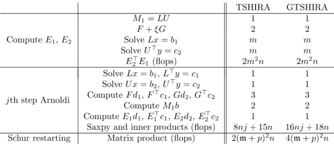
about half amount of the computation cost needed in GE SDA and GE SA. Our nu-merical results in Table 5 conﬁrm this observation. Finally, we summarize the process of applying TSHIRA/GTSHIRA to solve the GEP in (1) in Algorithm 7 and show the comparison of the computational costs for TSHIRA and GTSHIRA in Table 2.

4. Numerical results

In this section, we tests the above mentioned four types of structure preserving al-gorithms on computing the dispersion diagram of the frequency that are close to the stopping frequency of the SAW filter. The piezoelectric substrate of the filter is made of 15o rotated quartz. The configuration of our computational domain is shown in Figure 1 where the domain width AB and height CD are set to be 10−6and 3×10−6, respectively, the ratio of the electrode width EF versus the domain width is set to be1

2 and the ratio

of the electrode thickness DE versus the domain height is ₁₅1. In our numerical studies, the viscous damping coeﬃcient κ1is set to be 10−14and the mass damping coeﬃcient κ2

is taken as 1− κ1 to account for the eﬀect from the electrode weight. All computations

are carried out in MATLAB 2010b on a HP workstation with an Intel Quad-Core Xeon X5570 2.93GHz and 60 GB main memory, using IEEE double-precision ﬂoating-point

(18)

TSHIRA GTSHIRA Compute E1, E2 M1= LU 1 1 F + ξG 2 2 Solve Lx = b1 m m Solve U⊤y = c2 m m E₂⊤E1 (ﬂops) 2m2n 2m2n jth step Arnoldi Solve Lx = b1, L⊤y = c1 1 1 Solve U x = b2, U⊤y = c2 1 1 Compute F d1, F⊤c1, Gd2, G⊤c2 3 3 Compute M1b 2 2 Compute E1d1, E1⊤c1, E2d2, E2⊤c2 1 1

Saxpy and inner products (ﬂops) 8nj + 15n 16nj + 18n Schur restarting Matrix product (ﬂops) 2(m + p)2_n _{4(m + p)}2_n

Table 2: Computational costs for TSHIRA and GTSHIRA.

arithmetic.

Suppose m reciprocal pairs of eigenvalues near U are desired. For TSHIRA and GTSHIRA, the restart procedure will be activated when the desired eigenpairs don’t converge before the dimension of the Krylov subspace reaches 5m. This is done by setting the value of p in Step 4 of Algorithms 4 and 6 to 4m. In the following discussion, we take m = 5 and the matrix dimensions of Ci and Cbare n = 63960 and m = 723, respectively.

An example of computed reciprocal eigenpairs nearU at frequency ω = 1.2757/(2π)×1010

is shown in Figure 2. The dispersion diagrams of the attenuation constant α and the propagation constant β associated with the eigenvalue λ(ω) are shown in Figure 3, for frequency ω around the stopping band, where the eigenpair most close to −1 on the complex plane is plotted.

4.1. Accuracy of structure-preserving eigensolvers

In this subsection, we compare the accuracy of the eigenpairs, computed by structure-preserving Algorithms 1, 2 and 7, respectively, for the GEP (8). Recall that the Krylov subspace Uj generated by the⊤-Hamiltonian matrix B is automatically ⊤-isotropic in

Theorem 3.2, and the subspacesZjandYj+1generated in Theorem 3.4 are automatically ⊤-bi-isotropic. As mentioned in Subsections 3.3 and 3.4, isotropic re-orthogonalization in

Step 3 of Algorithm 3 and Steps 5 and 5 of Algorithm 5 is important in maintaining the

⊤-isotropic property. Moreover, Theorem 3.3 and 3.5 both show that the multiplicities

of eigenvalues of (K, N ) are all even. In other words, no duplicate eigenpairs need to be computed theoretically when the⊤-isotropic property is kept during the computation. On the other hand, without the isotropic re-orthogonalization process, extra computa-tion cost can arise in computing the duplicate eigenpairs. We would like to address this issue by numerical studies shown in the following. We also like to point out that the accuracy of the computed eigenpairs can be aﬀected by diﬀerent approaches in isotropic re-orthogonalization.

(19)

−1 −0.8 −0.6 −0.4 −0.2 0 0.2 0.4 0.6 0.8 1 −1 −0.9 −0.8 −0.7 −0.6 −0.5 −0.4 −0.3 −0.2 −0.1 0 0.1 λ₁(ω) λ₂(ω) λ₃(ω) λ₄(ω) λ₅(ω)

real part of eigenvalues

imaginary part of eigenvalues

Figure 2: The distribution of the eigenvalues which are close to and inside ofU.

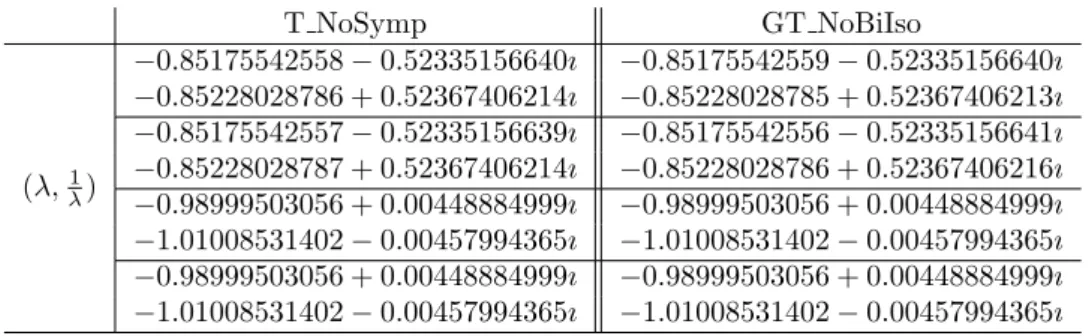
First, let us denote the algorithm that applying TSHIRA without the re-symplectic process as T NoSymp and the algorithm that applying GTSHIRA without these re-bi-isotropic processes as GT NoBiIso. In Table 3, the convergent eigenvalues obtained by T NoSymp and GT NoBiIso at frequency ω = 1.2757/(2π)× 1010_{are listed. Obviously,}

one can see that, in case only two eigenpairs{(λ1, λ−11 ), (λ2, λ−12 )} are needed here, the

algorithms T NoSymp and GT NoBiIso return four convergent eigenpairs in which two of them are indeed the duplicated pairs.

T NoSymp GT NoBiIso (λ,1_λ) −0.85175542558 − 0.52335156640ı −0.85175542559 − 0.52335156640ı −0.85228028786 + 0.52367406214ı −0.85228028785 + 0.52367406213ı −0.85175542557 − 0.52335156639ı −0.85175542556 − 0.52335156641ı −0.85228028787 + 0.52367406214ı −0.85228028786 + 0.52367406216ı −0.98999503056 + 0.00448884999ı −0.98999503056 + 0.00448884999ı −1.01008531402 − 0.00457994365ı −1.01008531402 − 0.00457994365ı −0.98999503056 + 0.00448884999ı −0.98999503056 + 0.00448884999ı −1.01008531402 − 0.00457994365ı −1.01008531402 − 0.00457994365ı

Table 3: Convergent eigenvalues computed by T NoSymp and GT NoBiIso at ω = 1.2757/(2π)× 1010_.

Next, let’s compare the accuracy of the computed eigenpairs obtained from three diﬀerent isotropic re-orthogonalization approaches in GTSHIRA. One or two steps of re-bi-isotropic process can be performed by the for-loops in Steps 5-5 and 5-5.

To distinguish among various re-bi-isotropic processes, we use notations “FullIso”, “zIsoY” and “yIsoZ” deﬁned as follows:

• FullIso: Algorithm 5 with two for-loops in Steps 5-5 and 5-5.

(20)

−0.2 −0.15 −0.1 −0.05 0 0.05 0.1 0.15 0.2 1.85 1.9 1.95 2 2.05 x 109 α ω 0.95 1 1.05 1.85 1.9 1.95 2 2.05 x 109 β / π ω

Figure 3: Dispersion diagrams of α and β near the stopping band.

• yIsoZ: Algorithm 5 with one for-loop in Steps 5-5 and omitting for-loop in Steps 5-5.

To measure the accuracy of computed eigenpairs of (8), we consider the relative residual of an eigenpair (λ, ψ) where ψ = [ψ⊤_i , ψ⊤_ℓ]⊤ which is deﬁned as following:

[ Ci Ciℓ C_ir⊤ 0 ] ψ− λ [ 0 Cir C_iℓ⊤ Cb ] ψ F [ Ci Ciℓ C_ir⊤ 0 ] F ∥ψ∥F+|λ| [ 0 Cir C_iℓ⊤ Cb ] F ∥ψ∥F ,

here∥ ∗ ∥F is the Frobenius matrix norm. The relative residuals of the convergent

eigen-pairs computed by “FullIso”, “zIsoY” and “yIsoZ” are shown in Figure 4. From the numerical results in Figure 4, we see that the accuracy of the convergent eigenpairs computed by “yIsoZ” is higher than those by “FullIso” and “zIsoY”. This result can be explained from the accumulation of the errors in the equalities (18) and (19). Let

ξj,K ≡ ∥ bKZj− YjHbj− bhj+1,jyj+1ej⊤∥2 and ξj,N ≡ ∥ bN Zj− YjRbj∥2, denote these errors

in the jth iteration. The error ξj,N depends on the accuracy of the solution of the linear

systems in (23). If zj is reorthogonalized to J ¯Yj, then the error produced by this

re-orthogonization will reduce the accuracy of ξj,N. Therefore, ξj,N produced by “FullIso”

and “zIsoY” are greater than that by “yIsoZ” as shown in Figure 5.(a). On the other hand, the error ξj,K only depends on the accuracy of matrix product vector and vector

inner product. Obviously, the amount of ξj,K is much less than the amount of ξj,N.

Consequently, even though the accuracy of ξj,Kcan reduced by the errors from

reorthog-onalization yj+1 toJ ¯Zj as shown Figure 5.(b), the reorthogonalization process “yIsoZ”

is much accurate than the “FullIso” and “zIsoY” reorthogonalization processes.

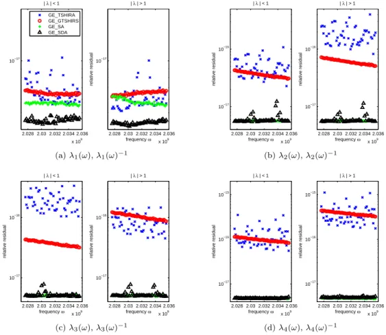
Finally, we compare the accuracy of the eigenpairs (λ(ω), u(ω)) obtained from GE SDA, GE SA, GE TSHIRA and GE GTSHIRA with ”yIsoZ” re-bi-isotropic process. The rel-ative residuals resulted from these algorithms in computing four reciprocal eigenpairs

(21)

T5 T4 T3 T2 T1 T6 T7 T8 T9 T10 10−18 10−16 10−14 10−12 10−10 eigenvalue relative residual zIsoY FullIso yIsoZ

Figure 4: The relative residual of the computed eigenpairs produced by diﬀerent re-bi-isotropic processes in Algorithm 5 with shift value τ =−0.99.

in Figure 6 for each frequency ω near the stopping band. Obviously, one can see that the accuracy of the eigenpairs obtained from GE SDA and GE SA are higher than those obtained by GE TSHIRA and GE GTSHIRA.

4.2. Comparison with computational costs

In this subsection, we discuss the computational costs of structure-preserving Algo-rithms 1, 2 and 7 in computing m = 5 desired eigenpairs. Our numerical results show that the desired eigenpairs are convergent within 5m⊤-isotropic Arnoldi steps without restart for GE TSHIRA and GE GTSHIRA. On the other hand, it requires total 18 iterations to obtain a convergent Xk in Steps 3.1-3.1 for the SDA algorithm. As we

mentioned in Subsection 3.3, the number of forward and backward substitutions needed for GE TSHIRA and GE GTSHIRA is only about half the amount of these substitutions that needed to transform the GEP into TPQEP in GE SDA and GE SA. Since only ad-ditional 25 forward substitutions and backward substitutions are needed in GE TSHIRA and GE GTSHIRA for solving linear systems Lx = b and U y = c, we expect GE TSHIRA and GE GTSHIRA to be more robust than GE SA and GE SDA. The following numer-ical results support this observation.

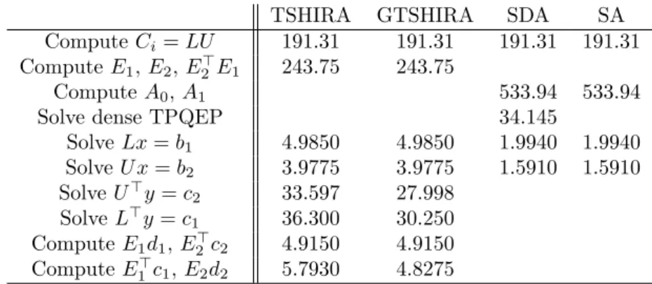
To give an overall comparison for GE SDA, GE SP, GE TSHIRA and GE GTSHIRA, in Table 4, computational intensive items in these algorithms are listed in the ﬁrst column and the sums of the CPU times for each associated item are listed in the other four columns. From the results in Table 4, the dominant computational costs in GE TSHIRA and GE GTSHIRA are the costs for computing E1, E2, E2⊤E1 and LU factorization of

Ci. For GE SDA and GE SA, the cost in computing the matrices A0 and A1 of the

TPQEP is the main cost comparing to the other costs. Obviously, the numbers shown in Table 4 indicate that GE TSHIRA and GE GTSHIRA are more eﬃcient than GE SDA and GE SA. We also plot the overall CPU times for GE SDA and GE GTSHIRA with

(22)

0 5 10 15 20 25 10−18 10−16 10−14 10−12 10−10 10−8 10−6 j−th step || N Z j − Y j R j ||2 zIsoY FullIso yIsoZ (a)∥ bN Zj− YjRbj∥2 0 5 10 15 20 25 10−18 10−16 10−14 10−12 10−10 10−8 10−6 j−th step || K Z j − Y j H j −h j+1,j yj+1 ej T || 2 zIsoY FullIso yIsoZ (b)∥ bKZj− YjHbj− bhj+1,jyj+1e⊤j∥2

Figure 5: The errors of the equalities in (18) and (19) for “FullIso”, “zIsoY” and “yIsoZ”.

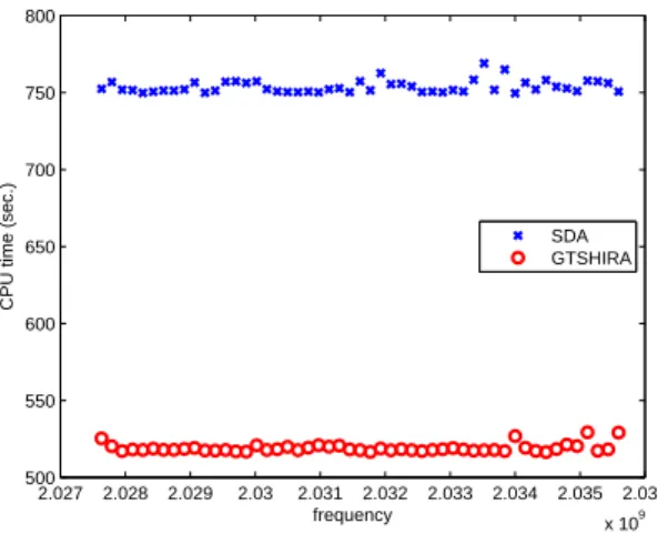
frequency from 1.274/(2π)× 1010 to 1.279/(2π)× 1010in Figure 7. From Figure 7, one can see that the total CPU times needed in GE SDA and GE SA are 40% more than the CPU time needed in GE TSHIRA and GE GTSHIRA for computing 5 desired eigepairs.

TSHIRA GTSHIRA SDA SA Compute Ci= LU 191.31 191.31 191.31 191.31

Compute E1, E2, E2⊤E1 243.75 243.75

Compute A0, A1 533.94 533.94

Solve dense TPQEP 34.145

Solve Lx = b1 4.9850 4.9850 1.9940 1.9940 Solve U x = b2 3.9775 3.9775 1.5910 1.5910 Solve U⊤y = c2 33.597 27.998 Solve L⊤y = c1 36.300 30.250 Compute E1d1, E2⊤c2 4.9150 4.9150 Compute E₁⊤c1, E2d2 5.7930 4.8275

Table 4: CPU times (sec.) for GE TSHIRA, GE GTSHIRA, GE SDA and GE SA.

5. Conclusion

In this paper, we have discussed the structure-preserving methods for solving the generalized eigenvalue problem arising in the surface acoustic wave propagation on a simple resonator with an interdigital transducer (IDT) where electrodes are arranged periodically on piezoelectric substrates (PZT) such as 15o _{rotated Quartz. With given}

periodic boundary conditions, the eigenvalues of the GEP appear in the reciprocal pairs (λ, λ−1). In order to preserve the reciprocal relationship of the eigenvalues, the GEP

(23)

2.028 2.03 2.032 2.034 2.036 x 109 10−17 | λ | < 1 2.028 2.03 2.032 2.034 2.036 x 109 10−17 | λ | > 1 frequency ω relative residual GE_TSHIRA GE_GTSHIRS GE_SA GE_SDA (a) λ1(ω), λ1(ω)−1 2.028 2.03 2.032 2.034 2.036 x 109 10−17 10−16 | λ | < 1 frequency ω relative residual 2.028 2.03 2.032 2.034 2.036 x 109 10−17 10−16 | λ | > 1 frequency ω relative residual (b) λ2(ω), λ2(ω)−1 2.028 2.03 2.032 2.034 2.036 x 109 10−17 10−16 | λ | < 1 frequency ω relative residual 2.028 2.03 2.032 2.034 2.036 x 109 10−17 10−16 | λ | > 1 frequency ω relative residual (c) λ3(ω), λ3(ω)−1 2.028 2.03 2.032 2.034 2.036 x 109 10−17 10−16 10−15 | λ | < 1 frequency ω relative residual 2.028 2.03 2.032 2.034 2.036 x 109 10−17 10−16 10−15 | λ | > 1 frequency ω relative residual (d) λ4(ω), λ4(ω)−1

Figure 6: Relative residuals for GE SDA, GE SA, GE TSHIRA and GE GTSHIRA with shift value

τ =−0.89.

large coefficient matrices and the other with small coefficient matrices. The structure-preserving algorithms GE SDA and GE SA in Algorithms 1, 2 are employed to solve the TPQEP (3) with small-size coefficient matrices and GE TSHIRA and GE GTSHIRA in Algorithms 7 are employed to solve the TPQEP (4) with large-size coefficient matrices.

In finding the five eigenpairs that are nearU and close to -1, we observed duplicate eigenpairs appear when applying GE TSHIRA and GE GTSHIRA without re-symplectic and re-bi-isotropic processes, respectively. On the other hand, no duplicate eigenpairs are observed when re-sympletic and re-bi-isotropic processes are integrated in GE TSHIRA and GE GTSHIRA. Three different re-bi-isotropic processes in GE GTSHIRA has been tested. We have found that using the re-bi-isotropic processes in Steps 5-5 of Algorithm 5 achieves the best accuracy. Moreover, our numerical results show that the relative resid-uals of the eigenpairs produced by GE SDA/GE SA and GE TSHIRA/GE GTSHIRA can be less than 10−17 and 10−15, respectively. Although the accuracy of GE SDA

(24)

2.027 2.028 2.029 2.03 2.031 2.032 2.033 2.034 2.035 2.036 x 109 500 550 600 650 700 750 800 frequency

CPU time (sec.)

SDA GTSHIRA

Figure 7: CPU times for GE SDA and GE GTSHIRA.

and GE SA is marginally higher than that of GE TSHIRA and GE GTSHIRA, we fur-ther found that the total CPU times required for computing the five desired eigepairs by GE SDA and GE SA are about 40% more than that are required by GE TSHIRA and GE GTSHIRA. Therefore, by transforming the GEP into the TPQEP (4), the structure-preserving Arnoldi type algorithm GE TSHIRA or GE GTSHIRA with one ”re-sympletic” or ” re-bi-isotropic” processes provide an accurate and efficient way in finding the reciprocal eigenpairs of the GEP (1).

Acknowledgments

This work is partially supported by the National Science Council and the National Center for Theoretical Sciences in Taiwan. The author Chin-Tien Wu like to thank the support from National Science Council under the grant number 99-2115-M-009-001.

References

[1] H. Allik and T. Hughes. Finite element method for piezoelectric vibration. Int. J. Numer. Methods

Eng., 2:151–157, 1970.

[2] M. B. Angel, M. I. Rocha-Gaso, M. I. Carmen, and A.V. Antonio. Surface generated acoustic wave biosensors for detection of pathogens: A review. Sensors, 9:5740–5769, 2009.

[3] M. Buchner, W. Ruile, A. Dietz, and R. Dill. FEM analysis of the reflection coefficient of SAWS in an infinite periodic array. In Proc. IEEE Ultrason. Symp., 371-375, 1991.

[4] C. K. Campbell. Surface Acoustic Wave Devices for Mobile and Wireless Communications. Aca-demic Press, INC., 1998.

[5] E. K.-W. Chu, T.-M. Hwang, W.-W. Lin, and C.-T. Wu. Vibration of fast trains, palindromic eigen-value problems and structure-preserving doubling algorithms. J. Comput. Appl. Math., 219:237–252, 2008.

[6] W. W. Lin E. K. Chu, T. M. Huang and C. T. Wu. Palindromic eigenvalue problems: a brief survey.

(25)

[7] A Hilliges, C. Mehl, and V. Mehrmann. On the solution of palindramic eigenvalue problems. In

Pro-ceedings 4th European Congress on Computational Methods in Applied Sciences and Engineering (ECCOMAS), Jyv¨askyl¨a, Finland, 2004.

[8] T.-M. Huang, W.-W. Lin, and J. Qian. Structure-preserving algorithms for palindromic quadratic eigenvalue problems arising from vibration on fast trains. SIAM J. Matrix Anal. Appl., 30:1566– 1592, 2009.

[9] T.-M. Huang, W.-W. Lin, and C.-T. Wu. Structure-preserving Arnoldi-type algorithms for solving palindromic quadratic eigenvalue problems in leaky surface wave propagation. Technical report, National Center for Theoretical Sciences, National Tsing Hua University, Taiwan, Preprints in Mathematics 2011-2-001, 2011.

[10] M. Koshiba, S. Mitobe, and M. Suzuki. Finite-element solution of periodic waveguides for acoustic waves. IEEE Trans. Ultrason. Ferroelectr. Freq. Control, 34, No. 4:472–477, 1987.

[11] R. Lerch. Simulation of piezoelectric devices by two- and three-dimensional ﬁnite elements. IEEE

Trans. Ultrason. Ferroelectr. Freq. Control, 37, No. 2:1990, 1990.

[12] W.-W. Lin. A new method for computing the closed-loop eigenvalues of a discrete-time algebraic Riccatic equation. Linear Alg. Appl., 96:157–180, 1987.

[13] D.S. Mackey, N. Mackey, C. Mehl, and V. Mehrmann. Structured polynomial eigenvalue problems: Good vibrations from good linearizations. SIAM J. Matrix Anal. Appl., 28:1029–1051, 2006. [14] D.S. Mackey, N. Mackey, C. Mehl, and V. Mehrmann. Vector spaces of linearizations for matrix

polynomials. SIAM J. Matrix Anal. Appl., 28:971–1004, 2006.

[15] V. Mehrmann and D. Watkins. Structure-preserving methods for computing eigenpairs of large sparse skew-Hamiltonian/Hamiltonian pencils. SIAM J. Sci. Comput., 22:1905–1925, 2001. [16] M. Mohamed, EL Gowini, and W. A. Moussa. A ﬁnite element model of a mems-based surface

acoustic wave hydrongen sensor. Sensors, 10:1232–1250, 2010.

[17] R. V. Patel. On computing the eigenvalues of a symplectic pencil. Linear Alg. Appl., 188:591–611, 1993.

[18] C. Schr¨oder. A QR-like algorithm for the palindromic eigenvalue problem. Technical report, Preprint 388, TU Berlin, Matheon, Germany, 2007.

[19] C. Schr¨oder. URV decomposition based structured methods for palindromic and even eigenvalue problems. Technical report, Preprint 375, TU Berlin, MATHEON, Germany, 2007.

[20] G.W. Stewart. A Krylov–Schur algorithm for large eigenproblems. SIAM J. Matrix Anal. Appl., 23:601–614, 2001.

[21] G.W. Stewart. Addendum to “A Krylov–Schur algorithm for large eigenproblems”. SIAM J. Matrix

Anal. Appl., 24:599–601, 2002.

[22] S. Zaglmayr. Eigenvalue problems in saw-ﬁlter simulations. Diplomarbeit, Institute of Computa-tional Mathematics, Johannes Kepler University Linz, Linz, Austria, 2002.

(26)

Structure-Preserving Arnoldi-Type Algorithm for

Solving Eigenvalue Problems in Leaky Surface Wave

Propagation

Tsung-Ming Huanga_{, Wen-Wei Lin}b_{, Chin-Tien Wu}c,∗

a_{Department of Mathematics, National Taiwan Normal University, Taipei 116, Taiwan.}

E-mail: [email protected].

b_{Department of Mathematics, National Taiwan University, Taipei 106, Taiwan. E-mail:}

c_{Department of Applied Mathematics, National Chiao Tung University, Hsinchu 300,}

Taiwan. E-mail: [email protected].

Abstract

We study the generalized eigenvalue problems (GEP) arising from modeling leaky surface waves propagation in a acoustic resonator with infinitely many pe-riodically arranged interdigital transducers. The constitution equations are dis-cretized by finite element method with mesh refinement along the electrode in-terface and corners. The associated GEP is then transformed to a T-palindromic quadratic eigenvalue problem so that the eigenpairs can be accurately and ef-ficiently computed by using a structure-preserving algorithm incorporating a generalized T-skew-Hamiltonian implicity-restarted Arnoldi method. Our nu-merical results show that the eigenpairs produced by the proposed structure-preserving method not only preserve the reciprocal property but also possess high efficiency and accuracy.

Key words: Leaky SAW, structure-preserving, palindromic quadratic eigenvalue problem, GTSHIRA, mesh reﬁnement

1. Introduction

Waveguide devices have been widely used in controlling and interconnecting guided electromagnetic waves. Advances in the thin film technology and efficient transducers further encourage investigations on more sophisticated waveguide concepts in acoustic system. Acoustic wave guide devices are widely employed in applications including telecommunication filters [8, 25] and sensor technolo-gies [2]. One of the basic element in most acoustic wave filters is a resonator which generally consists of reflectors externally coupled through one or two interdigital transducers (IDT). The IDT is primarily made by depositing pe-riodical metallic grating electrodes on a piezoelectric film substrate as shown

(27)

in Figure 1(a). Extensive theoretical and experimental works have been done specially on the Rayleigh surface acoustic wave [4, 9, 24, 25]. Finite element simulations of piezoelectric devices in two dimension (2D) and three dimension (3D) have been studied by Allik, Koshiba, Lerch, Buchner, Mohamed and oth-ers etc., [1, 6, 17, 19]. In the ﬁlter design, it is important to know the stop band width and the center frequency fc of the ﬁlter where fc = vs/λs here vs

and λs are the wave velocity and wave length of the incident wave. The center

frequency and stop band width can visually be determined by plotting the dis-persion diagram in which an eigenvalue problem associated with each frequency in the search range has to be solved.

Due to slower propagation velocity of the Rayleigh SAW, ﬁlters based on Rayleigh SAW design are usually limited to an operational frequency range less than 1GHZ. For frequency higher than 1GHZ, more recent attention has been paid to the so-called leaky surface acoustic wave (LSAW) because of its faster propagation speed in crystal cuts such as 64oYX-LiNbO3and 36oYX-LiTaO3,

and higher electromechanical coupling and minimal propagation loss in crystal cuts such as 40o ∼ 42o YX-LiTaO3 [8]. Searching a better crystal cut among

various piezoelectric substrates (PZT) to increase LSAW velocity becomes one of the major issues in high frequency ﬁlter design. For each crystal cut, one has to solve many eigenvalue problems to plot the dispersion diagram. An eﬃcient and accurate algorithm for solving eigenvalue problem resulted from mathemat-ical model of a LSAW resonator is desired.

The eigenvalue problem obtained from the ﬁnite element modeling of the SAW or LSAW resonance can be represented as

[ M1 G F⊤ 0 ] [ ψi ψℓ ] + λ [ 0 F G⊤ M2 ] [ ψi ψℓ ] = 0, (1) where M₁⊤ = M1 ∈ Cn×n, M2⊤ = M2 ∈ Cm×m, F and G ∈ Cn×m with

m ≪ n, and the supscript “⊤” denotes the complex transpose. The scalar λ∈ C is called the eigenvalue of (1) and the nonzero vector[ ψ⊤_i ψ⊤_ℓ ]⊤ is the associated eigenvector. The generalized eigenvalue problem (GEP) (1) can be reformulated into a T-palindromic quadratic eigenvalue problem (TPQEP) of the form

P(λ)ψi≡ (λ2A⊤1 + λA0+ A1)ψi= 0 (2a)

with

A1⊤= F M2−1G⊤, A0= F M2−1F⊤+ GM2−1G⊤− M1. (2b)

By taking the transpose ofP(λ) in (2a) and multiplying it by 1/λ2_{it is easily}

seen that the eigenvalues ofP(λ) appear in reciprocal pairs (λ, 1/λ) (including 0 and∞).

(28)

The GEP (1) can be solved by traditional methods such as the QZ and Arnoldi method. However, the reciprocal property of the eigenvalues of (1) can be destroyed easily and large numerical errors can be generated in computation [16]. To remedy the drawback, we transform the GEP (1) into the TPQEP (2a) so that the desired eigenpairs can be computed by structure-preserving meth-ods [11, 13, 15, 21, 22, 29, 30]. For solving the TPQEP with small and dense coeﬃcient matrices A0 and A1, a structure-preserving doubling algorithm for

solving (2a) was developed in [11] via the computation of a solvent of a nonlinear matrix equation associated with (2a). Another structure-preserving algorithm based on (S + S−1)-transform [20] and Patel’s approach [27] was developed in [15]. For problems with large and sparse matrices A0 and A1, a

structure-preserving algorithm using the (S + S−1)-transform and the implicity-restarted shift-and-invert Arnoldi method was also developed for searching eigenvalues in a speciﬁed region of interests [15].

In this paper, we apply the generalized T-skew-Hamiltonian implicity-restarted Arnoldi method developed in [15] to solve the TPQEP (2a). Based on the shift-and-invert technique, the desired eigenpairs can be easily extracted. For solv-ing the linear systems, although the coeﬃcient matrices A0 and A1 in (2b) is

large but not sparse, we derive a new formula by using the Sherman-Morrison-Woodbury formula so that the corresponding linear system can be eﬃciently solved. Comparing with the traditional Arnoldi method, our proposed structure-preserving method not only preserve the reciprocal property but also possess high eﬃciency and accuracy.

This paper is organized as follows. We shall first introduce finite element modeling for a simple resonator in Section 2. In Section 3, we introduce the efficient structure-preserving algorithm to solve the large and sparse generalized eigenvalue problems resulted from our FEM model. Our numerical experiments in Section 4 show that the proposed structure-preserving algorithm for solving the GEP in (1) is efficient and accurate. Finally, we conclude the paper in Section 5.

2. Finite Element Model for SAW

In contrast to the well known Rayleigh waves which consists of partial lon-gitudinal waves and shear waves, the LSAW mainly propagates in the shear direction on the sagittal plane and is trapped at substrate surface and satis-ﬁes the stress free boundary condition on the surface. These properties allow one to reduce the general mode analysis in 3D to a 2D problem as shown in Figure 1(b) [28]. Furthermore, the boundary conditions for displacement can naturally be set to be rigid on the bottom boundary and stress-free on the top surface, and the boundary conditions for the electric potential can be set to be short-circuited for the electrodes on the top boundary and open-circuited else-where [10]. As proved in Auld’s book [4], these boundary conditions guarantee the mode orthogonality and further ensure the mode excitation is determined

(29)

(a) A standard conﬁguration of SAW res-onators

(b) A 2D model of a LSAW resonator on the sagittal plane

Figure 1:

by the applied traction force and potential on the free surface. Therefore, on the sagittal plane, the usual 2D mode analysis can be applied to analyze the LSAW on the resonators with IDTs. In the following, we only consider the LSAW resonator on a 2D plane (the sagittal plane associated with crystal cuts). To model the wave propagation in an inﬁnite domain with periodically ar-ranged electrodes, thanks to the Floquet-Bloch Theorem, one can reduce the problem to a single cell domain with one IDT by assuming the wave ψ is quasi-periodic of the form ψ(x1, x2) = ψp(x1, x2)e(α+iβ)x1 where x1is the wave

prop-agation direction, p is the length of the unit cell (i.e. the periodic interval), α and β are the attenuation and phase shifts along the wave propagation direc-tion, respectively, and ψp satisﬁes ψp(x1+ p, x2) = ψp(x1, x2). Let Ω denote

the PZT with a single IDT as shown in Figure 2, and Γland Γr denote the left

and right boundary segments of Ω. For the general anisotropic PZT substrates, under the assumption of linear piezoelectric coupling, the elastic and electric ﬁelds interact following the general material constitutions below

T = cES− e⊤E,

D = eS + εSE, (3)

where vectors T , S, D and E are the mechanical stress, strain, dielectric dis-placement and the electric ﬁeld, respectively, and the matrices cE, εS and e are the elasticity constant, dielectric constant and piezoelectric constant matrices measured at constant electric and constant strain ﬁelds at constant temperature. For various crystal cut of the PZT, the material constant matrices cE_{, ε}S _and e depend on the Euler angle θ of the cut. By applying the Bond strain

trans-formation matrix Nθ [5] and the usual coordinates transformation matrix Mθ

to the strain ﬁeld and electric ﬁeld, respectively, the material constant matrices for the cut angle θ can be obtained by