國立交通大學
電子工程學系 電子研究所
碩 士 論 文
iLap: 三維積體電路上減少直通矽穿孔數
目之迭代式層級感知分割演算法
iLap: Iterative Layer-Aware Partitioning Algorithm
for Through-Silicon Via Minimization in 3D ICs
研 究 生:劉揚翔
指導教授:黃俊達 博士
iLap: 三維積體電路上減少直通矽穿孔數目之
迭代式層級感知分割演算法
iLap: Iterative Layer-Aware Partitioning Algorithm
for Through-Silicon Via Minimization in 3D ICs
研 究 生:劉揚翔
Student: Yang-Hsiang Liu
指導教授:黃俊達 博士
Advisor: Dr. Juinn-Dar Huang
國立交通大學
電子工程學系 電子研究所
碩士論文
A Thesis
Submitted to Department of Electronics Engineering & Institute of Electronics College of Electrical & Computer Engineering
National Chiao Tung University in Partial Fulfillment of the Requirements
for the Degree of Master
in
Electronics Engineering & Institute of Electronics
August 2010
Hsinchu, Taiwan, Republic of China
iLap: 三維積體電路上減少直通矽穿孔數目之
迭代式層級感知分割演算法
研究生:劉揚翔 指導教授:黃俊達 博士 國立交通大學 電子工程學系 電子研究所碩士班摘 要
相較於二維積體電路,三維積體電路在垂直方向的整合在二維製程技術逐漸 面臨瓶頸的情況下提供了進一步提升效能的可能性。此整合技術允許將晶粒做多 層堆疊,利用直通矽穿孔(Through-silicon vias, TSVs)進行垂直方向的信號連 線。雖然直通矽穿孔被視可行的垂直連線方式,但也伴隨著所佔面積太大及製造 過程的良率和穩定度的問題,因此直通矽穿孔的數量在設計電路的過程中是很重 要的關鍵。在這篇論文裡,為了最小化直通矽穿孔的數量,我們提出兩種迭代式 三維層級感知分割演算法(iLap-2和iLap-k)。iLap-2重覆性地運用二路最小切割 演算法,將給定的設計電路從底層往上一層一層地擺放;同時也在不違反輸入及 輸出腳位必頇在晶片底層的限制下,進而改善三維的積體電路。iLap-k則是基於 iLap-2的演算法架構,將iLap-2的二路分割演算法核心用多路分割演算法取代 之,使其更能考慮全域的分佈狀況,而達到更好的效果。與其它已習知的方法比 較,實驗結果顯示iLap系列的作法在直通矽穿孔的總量和分佈上有相當大程度的 改善。以iLap-k為例,相較於以hMetis分割法能達到的最少直通矽穿孔數目, iLap-k能夠達到33%的改善;並且在直通矽穿孔的分佈上,iLap-k顯得更加平均而 不會集中在某一層。這項優點不管是針對特定用途而設計的特殊應用積體電路 (ASIC)或是規則型架構的電路來說,都可以減少面積以及資源上的損失。ii
iLap: Iterative Layer-Aware Partitioning
Algorithm for Through-Silicon Via
Minimization in 3D ICs
Student: Yang-Hsiang Liu Advisor: Dr. Juinn-Dar Huang
Department of Electronics Engineering & Institute of Electronics National Chiao Tung University
Abstract
As compared with two-dimensional (2D) ICs, three-dimensional (3D) integration is a breakthrough technology of growing importance that has the potential to offer significant performance and functional benefits. This emerging technology allows stacking multiple layers of dies and resolves the vertical connection issue by through-silicon vias (TSVs). However, though a TSV is considered a good solution for vertical connection, it also occupies significant silicon estate and incurs reliability problem. Because of these challenges, to minimize the number of TSVs becomes important in the design processes. Therefore, in this thesis, we propose two iterative layer-aware 3D partitioning algorithms, named iLap-2 and iLap-k, for TSV minimization. iLap-2 iteratively applies 2-way min-cut partitioning to gradually divide a given design layer by layer in the bottom-up fashion. Meanwhile, iLap-2 also properly fulfills a special I/O pad constraint incurred by 3D ICs to further improve its outcome. Based on iLap-2, iLap-k replaces the 2-way partitioning by k-way partitioning engine for considering the distribution of the future. The experimental results show that iLap-k can reduce the number of TSVs by about 33% as compared to several existing methods. Besides, iLap-k distributes TSVs more evenly among different vertical layers, preventing any layer junction from having a burst number of TSVs. That is important to application specific integrated circuit (ASIC) as well as regular structures.
誌 謝
首先要謝謝我的指導教授─黃俊達副教授,在碩士兩年當中,給予充份的時 間修習研究所相關專業課程,在每週實驗室會議上也不時地教導與鼓勵。在論文 研究上,更樂意安排個別會議時間,適時給予寶貴的意見及指導。並且在實驗室 的自由學習風氣下,培養出個人獨立思考問題以及解決問題的能力,也能學習到 與其它人的團體合作,對老師的感激之情,並非以簡短的文句可以表達。 再來我要感謝我的父母,從小一路栽培我到碩士畢業,讓我在沒有經濟壓力 的情況下,安心順利的念完所有的學程。也謝謝百忙之中來參加口試的委員們─ 黃婷婷教授、王廷基教授和張世杰教授,你們的意見指導讓我獲益良多,非常感 謝。 謝謝博士班的學長姐們,特別是嘉怡學姐和雅詩學姐,不僅是會議的上台報 告,還有論文撰寫,都能給予寶貴的經驗,讓我可以順利完成論文研究。還有實 驗室的同學─寶鑑、詣航和蜜祐,碩一時的一起努力參與程式競賽、修課、討論、 以及做實驗,對我來說都是很珍貴的回憶。最後,謝謝實驗室的學弟們─晧凌、 崇羽與瀚元,在口試時幫忙我打理一切,謝謝你們。 希望大家在未來的日子裡,都能順順利利完成自己的研究,也希望這篇論文 對科技的進步能有小小的貢獻,再次謝謝你們的幫忙。iv
Contents
摘 要 ...i Abstract ... ii 誌 謝 ... iii Contents ...ivList of Tables ...vi
List of Figures ... vii
Chapter 1 Introduction ... 1
1.1 3D Structures ... 2
1.2 Related Works ... 4
1.2.1 EV-Matrix ... 4
1.2.2 Multilevel Multilayer Partitioning Algorithm for 3D ICs ... 6
1.3 Thesis Organization ... 7
Chapter 2 Problem Description ... 8
2.1 Motivations ... 8 2.2 Problem Descriptions ... 11 2.2.1 Design Model ... 11 2.2.2 3D Architecture Model ... 11 2.2.3 TSV Calculation ... 12 2.2.4 Problem Formulation ... 13
Chapter 3 Proposed Algorithm ... 14
3.1 Iterative Unbalanced 2-Way Partitioning Framework... 14
3.1.1 Iterative Procedure ... 14
3.1.2 iLap-2... 17
3.1.3 Parasitical Area Problem ... 18
3.2 Iterative k-Way Partitioning Framework ... 20
3.2.1 The Reason to Use k-Way Partitioning Engine ... 20
Chapter 4 Experiments ... 25
4.1 Environment Setup ... 25
4.2 Results and Analyses ... 27
4.2.1 Analysis of TSV Count with Fixed Layer ... 27
4.2.2 TSV Count ... 29
4.2.3 Distribution of TSV Count ... 30
4.2.4 Runtimes ... 32
Chapter 5 Conclusion ... 33
vi
List of Tables
Table 1. 14 test cases. ... 26 Table 2. Total number of TSVs when k = 4. ... 28 Table 3. Total number of TSVs when k = 8. ... 28
List of Figures
Figure 1. Relative delay vs. process technology. ... 1
Figure 2. A TSV-based 3D structure. ... 2
Figure 3. Reduce the length of the global connections by TSVs. ... 3
Figure 4. The area overhead of TSVs. ... 3
Figure 5. A partitioned graph. ... 5
Figure 6. EV-matrix. ... 5
Figure 7. The flow of multilevel multilayer partitioning algorithm. ... 6
Figure 8. A 4-layer 3D partitioning example. ... 9
Figure 9. Different maximum cuts with the same total number of TSVs. ... 10
Figure 10. An example of the 3D model. ... 13
Figure 11. Compact fixed cells into a supervertex. ... 15
Figure 12. Unbalanced 2-way partitioning. ... 15
Figure 13. L1 compaction. ... 16
Figure 14. L2 decision. ... 16
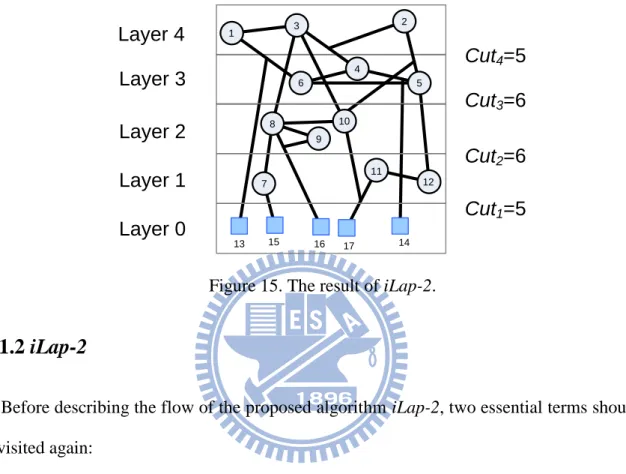
Figure 15. The result of iLap-2... 17
Figure 16. The flow and pseudo code of iLap-2. ... 18
Figure 17. Area Problems on top-most layers. ... 18
Figure 18. An example for different area ratio. ... 20
Figure 19. A 4-layer example for the local decision of iLap-2. ... 21
Figure 20. Different results in k-way partitioning. ... 22
viii
Figure 22. The flow and pseudo code of iLap-k. ... 23
Figure 23. Classification of 3D partitioning. ... 25
Figure 24. The number of required TSVs in 3D ICs. ... 29
Figure 25. Normalized TSV count. ... 30
Figure 26. Standard deviation of TSV count. ... 31
Figure 27. Maximum TSV ... 31
Chapter 1 Introduction
With the advance of semiconductor manufacturing process technology, ever-shrinking feature size and exponentially growing number of transistors on a chip are facing severe and alarming challenges such as signal integrity, power integrity and dissipation, leakage power, clock distribution and yield issues [1]. Besides, the wire delay becomes more important than gate delay [2]. As shown in Figure 1, the long interconnect delay fails to shrink as the device delay does and eventually dominates the system performance in the system-on-chip era. Therefore, a solution is demanded to both alleviate the interconnect speed bottleneck and provide new avenues for the advanced device and architectural innovation. As approaching the physical limitation, traditional scaling is no longer the only way for advancing manufacturing process technology and hence three-dimensional (3D) technologies are emerging in recent years [3]–[10]. 3D integrated circuit (3D IC) technologies enable to stack multiple dies on a single chip and provide three unique advantages compared to conventional 2D approaches, namely higher system integration, better heterogeneous integration, and shorter global interconnect length.
1.1 3D Structures
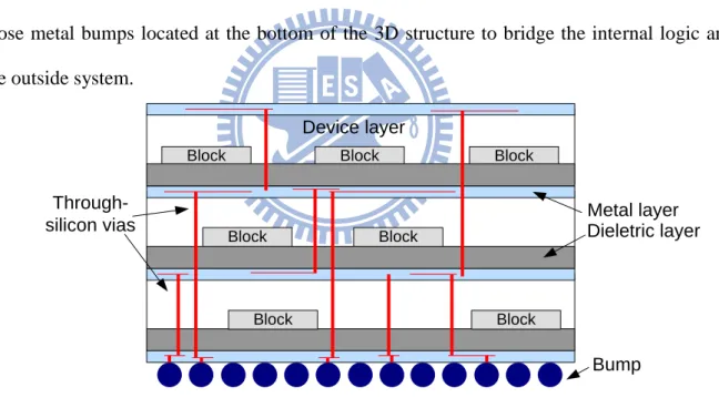
Among those state-of-the-art 3D integration technologies, the wire bonding method is preferred in the system-in-package (SiP) process to accomplish the vertical interconnect between different layers [3]–[5]. However, terminals of chips have to be arranged at the periphery of the chips. Therefore, the wire bonding technique is difficult for high vertical interconnections because the number of the vertical connections is limited. Another promising technology is using the Through-Silicon Via (TSV) [6]–[10]. Figure 2 illustrates a typical TSV-based 3D IC structure. TSVs cut across thinned silicon substrates to make inter-die connections, allowing high compatibility with the present standard CMOS process. The position of TSVs can be inside of chips. Besides, all external I/O signals must go through those metal bumps located at the bottom of the 3D structure to bridge the internal logic and the outside system.
Block Block Block
Block Block Block Block Metal layer Device layer Dieletric layer Bump Through-silicon vias
Figure 2. A TSV-based 3D structure.
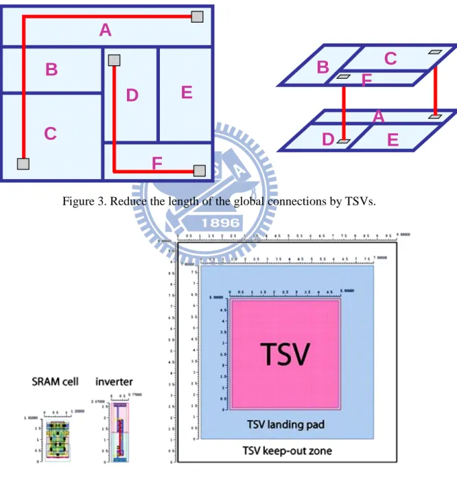
Nevertheless, compared with a standard 2D process, though the TSV-based vertical transmission can theoretically be fast by reducing the global connections as shown in Figure 3, currently available processes for TSV fabrication suffer relatively low yield [11] as well as large area overhead [12]–[14]. Figure 4 shows the area overhead of the TSVs, compared to the other operation cells, it is huge obviously. The area of a single TSV is 64um2 (2012); however, a 6-transistor SRAM occupies 0.061um2. We can calculate the area ratio from TSVs
to the SRAM is about 1049 [1]. Therefore, the area overhead is important to ASIC or some regular structures. There are some researches about TSVs in the back-end processes considering timing and thermal issues already [15]–[17]. In summary, using less number of TSVs is highly desirable both for improving the yield of 3D design and for minimizing the area overhead. Consequently, the issue of TSV minimization must be well addressed as stepping into the 3D IC arena.
A
B
C
D
E
F
A
D
E
B
C
F
Figure 3. Reduce the length of the global connections by TSVs.
1.2 Related Works
In general, how a design gets partitioned into different vertical layers of a 3D logic structure basically determines how many TSVs are mandatory for signal connection among those vertical layers. In the past few years, several previous works have already been proposed to tackle the problem of 3D partitioning for TSV minimization. One solution is to model the problem as an integer linear programming (ILP) problem [18], however, whose runtime grows exponentially as problem size increases. In [19][20], each of them develops a modified FM-based [21] partitioning method to obtain the resultant layer assignment aggregately at a time, not layer by layer. For this layer-aware algorithm, there is a brief introduction in the later section about [19] proposed on ISQED 2010. Meanwhile, the authors of 3D FPGA synthesis frameworks TPR [22]–[24] and MEANDER [25][26] alternatively use a two-step approach – first applying the well-known partitioning algorithm hMetis [27][28] to divide a design into layer-unaware partitions, and then assigning each partition to its target layer – to accomplish 3D design partitioning. In MEANDER, the authors assign each part to layer randomly, while EV-matrix [22] is used in TPR. We will detail how it runs a few simple and easy steps to minimize the number of TSVs in the next section.
From these related works, we can figure out the importance to the partitioning process. Because it is the first step to translate the 2D netlist into the 3D structure, the partitioning result directly influences the number of TSVs seriously. In our work, we try to use a layer-aware algorithm to iteratively minimize the number of TSVs.
1.2.1 EV-Matrix
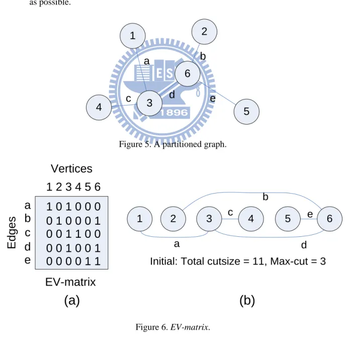
Here we introduce a linear-placement method doing layer assignment after a min-cut partitioning in TPR [23]. It uses an EV-matrix [22] to model the 3D structure. After a min-cut partitioning like Figure 5, the graph is mapped into an EV-matrix as Figure 6(a). It is an m × n
matrix where m (the number of rows) is the number of edges in the graph and n (the number of columns) is the number of parts. An element a(i, j) = 1 in the matrix is nonzero if the j-th part is a terminal of the i-th net. If a part is not a terminal for a net, the corresponding
EV-matrix element is 0. The bandwidth of a matrix is defined as the maximum distance
between the first and last nonzero entries among all rows. In other words, the bandwidth is associated to the number of cuts of each edge in Figure 6(b). There are two goals:
i) To minimize the total cuts: it makes the bandwidth as small as possible on each row. ii) To minimize the maximum cut size: it makes all of the 1’s as closed the main diagonal
as possible.
1
2
3
4
5
6
a
b
c
d
e
A partitioned graph
Figure 5. A partitioned graph.
1 0 1 0 0 0
0 1 0 0 0 1
0 0 1 1 0 0
0 0 1 0 0 1
0 0 0 0 1 1
a
b
c
d
e
1 2 3 4 5 6
Vertices
E
d
g
e
s
EV-matrix
1
2
3
4
5
6
a
b
c
d
e
Initial: Total cutsize = 11, Max-cut = 3
(a)
(b)
In order to complete the objective, it only needs to move columns and rows. Although it is effective in time, it still has some disadvantages. Firstly, it cannot provide a good solution especially in hypergraph. Secondly, though hMetis is an efficient and effective min-cut multi-way partitioning tool, it lacks for layer-aware concept. That is, a typical 2D partitioning algorithm basically gives a similar weight to a cut between any two partitions, while that weight can be very different in 3D partitioning and highly depends on whether those two partitions (i.e., layers) are closed or far away from each other. Hence, the layer-unaware algorithms usually fall into the local minimum solution.
1.2.2 Multilevel Multilayer Partitioning Algorithm for 3D ICs
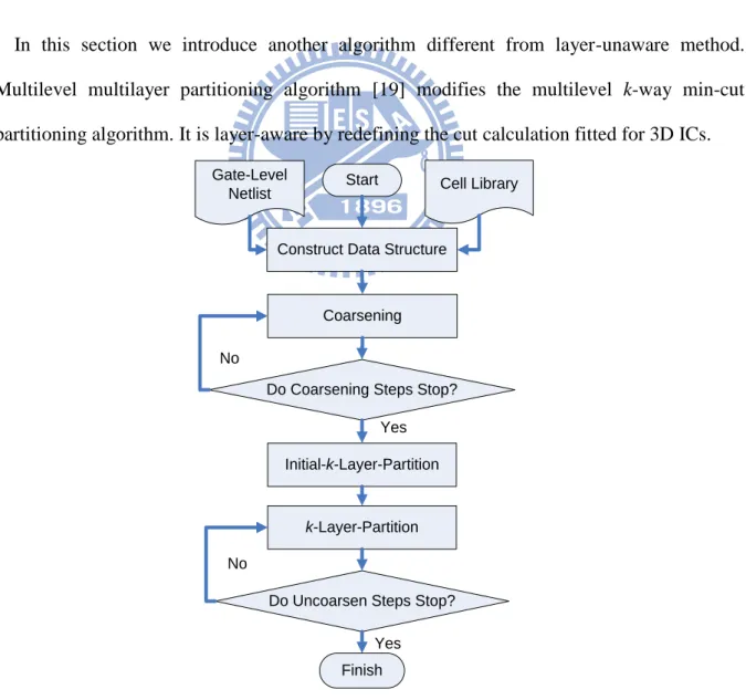
In this section we introduce another algorithm different from layer-unaware method. Multilevel multilayer partitioning algorithm [19] modifies the multilevel k-way min-cut partitioning algorithm. It is layer-aware by redefining the cut calculation fitted for 3D ICs.
Gate-Level Netlist
Construct Data Structure
Do Coarsening Steps Stop?
Start Cell Library
Coarsening
Initial-k-Layer-Partition
k-Layer-Partition
Do Uncoarsen Steps Stop?
Finish Yes
Yes No
No
Figure 7 is the overall flow of this algorithm. At the beginning, the coarsening phase clusters the cells with high connectivity together. And then, do a k-layer partitioning to initialize the locations of all the gates. After the initial partitioning phase, repeat k-layer partitioning and uncoarsening to refine the total number of cuts required until the uncoarsening steps stop.
Note that this framework performs one multilevel iteration to decide which layer all of the gates should be placed. It reduces only the total number of TSVs without considering the maximum number of TSVs among all of the adjacent layers. Although this work is sensitive to the 3D structure, it is not good enough to find the solution.
Therefore, in this thesis, we propose an iterative layer-aware partitioning algorithm, named
iLap, for TSV minimization in 3D ICs. Unlike [18]–[20], iLap merely identifies a layer at
each iteration, i.e., iLap is iterative and gradually produces the final result layer by layer. Also unlike [22]–[26], which perform layer-unaware partitioning then layering, iLap applies layer-aware partitioning at each iteration. Though iLap also utilizes min-cut partitioning as the kernel of its engine, the experiment results demonstrate that iLap can apparently do better TSV minimization than three other hMetis-based and the multilevel multilayer partitioning methods for various number of layers and the required runtime is just within few seconds. Moreover, in addition to TSV minimization, iLap can also distribute TSVs among layers more evenly than other existing arts. This feature is considered a big plus in design flows for ASIC as well as for other 3D regular logic structures (e.g., 3D FPGAs).
1.3 Thesis Organization
The organization of this thesis is as follows. In Chapter 2, we briefly introduce our motivations and the problem formulation. Chapter 3 details the proposed iterative layer-aware partitioning algorithm. The experimental results and analyses are reported in Chapter 4.
Chapter 2 Problem Description
This chapter describes the motivations and the problem formulation. We introduce the reasons why to develop a new partitioning algorithm fitted for 3D ICs technology and how to calculate the number of TSVs for the 3D model.
2.1 Motivations
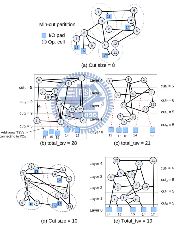
In 3D ICs, nets crossing multiple layers (or tiers) need vertical inter-layer connections. In general, vertical connections are commonly achieved utilizing TSVs, which go through device layers, connecting the pins of the same net distributed on different device layers. It has been reported that vertical connections implemented using TSVs greatly affect area and reliability of 3D ICs [11]. As a result, it is very important to minimize the TSV usage while performing 3D design partitioning (or layering). Figure 8 demonstrates a simple example of the 4-layer 3D partitioning. A given design with its 4-way min-cut partitioning result is presented in Figure 8(a). Figure 8(b) and (c) present two different 3D layering outcomes based on the same partitioning result given in Figure 8(a) but two various layer assignments. From the observations on Figure 8, we have to highlight three ideas. Firstly, as previously mentioned, all external I/O pads (i.e., bumps) must be located at the bottom-most layer (i.e., Layer 0 in Figure 8). That is, those vertices connected to I/O pads are likely to introduce extra TSVs for correctly connecting to bumps located at Layer 0. As shown in Figure 8(b), five extra connections (in red dotted line) suggest that 13 more TSVs are required, which are generally ignored in conventional multi-way min-cut partitioning algorithms. It also explains why there is a big difference between the total cut size (=8) in Figure 8(a) and the number of total TSVs (=28) in Figure 8(b). Secondly, different layer assignments result in different TSV requirements even the initial partitioning result is identical. For instance, the number of TSVs reduces from 28 in Figure 8(b) to 21 in Figure 8(c) simply because the permutation of
partitions is changed. Finally, because min-cut partitioning does not aware the 3D architecture, it might not produce the global solution even though exhaustively examining all possible layer permutations. For example, the cut size in Figure 8(d) is more than Figure 8(a), but it requires only 19 TSVs in Figure 8 (e) smaller than the best permutation in Figure 8 (c).
Layer 1 Layer 2 Layer 3 Layer 4 Layer 0 12 11 10 9 8 7 2 5 1 4 3 6 13 14 15 16 17 I/O pad Op. cell 15 2 5 4 1 6 3 12 11 10 9 8 7 13 16 14 17 2 5 4 1 6 3 12 11 10 9 8 7 15 13 16 14 17 Additional TSVs connecting to I/Os (b) total_tsv = 28 (c) total_tsv = 21 (a) Cut size = 8
2 1 3 5 4 6 10 9 8 12 11 7 13 14 15 16 17 12 11 10 9 8 7 2 5 1 4 3 6 13 15 16 14 17 cut3 = 4 cut2 = 5 cut1 = 5 cut0 = 5 Layer 1 Layer 2 Layer 3 Layer 4 Layer 0
(d) Cut size = 10 (e) Total_tsv = 19
cut3 = 5 cut2 = 6 cut1 = 5 cut0 = 5 cut3 = 5 cut2 = 9 cut1 = 9 cut0 = 5 Min-cut paritition e1
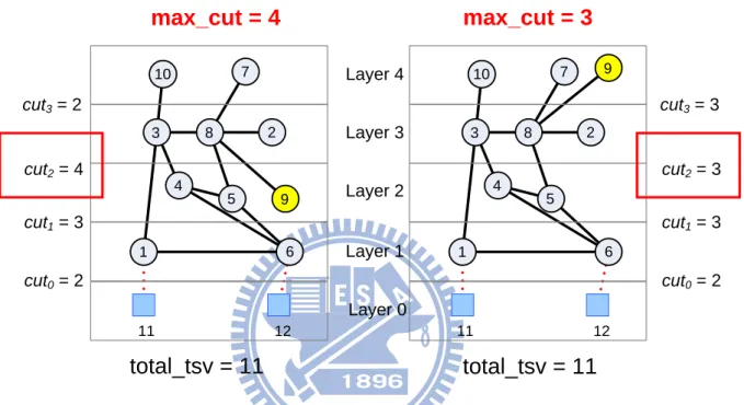
Through the multilevel multilayer partitioning algorithm [19] is layer-aware, it ends the algorithm just in one multilevel iteration without considering the maximum number of TSVs between the adjacent layers. Figure 9 shows the different maximum cuts with the same total number of TSVs. For some regular structures with fixed resources, the design circuit with excess cuts might not be successfully implemented.
5 4 1 6 3 10 9 8 7 2 cut3 = 2 cut2 = 4 cut1 = 3 cut0 = 2 11 12 5 4 1 6 3 10 9 8 7 2 cut3 = 3 cut2 = 3 cut1 = 3 cut0 = 2 11 12 Layer 1 Layer 2 Layer 3 Layer 4 Layer 0
total_tsv = 11
total_tsv = 11
max_cut = 4
max_cut = 3
Figure 9. Different maximum cuts with the same total number of TSVs.
According to the huge area overhead of TSVs mentioned before, the number of TSVs directly reflects the area cost. Hence, in order to reduce the extra area introduced by TSVs under 3D structures, we can minimize the number of TSVs.
Based on the above discussions, it should be clear that conventional multi-way min-cut partitioning algorithms virtually have no chance to perform 3D partitioning well in their original forms due to their ignorance about the vertical layout structure. Even though the other exact algorithms are layer-aware, they still can not efficiently find a good mapping for 3D ICs. Therefore, a layer-aware partitioning algorithm simultaneously considering the total number of TSVs and maximum number of TSVs between the adjacent layers specifically
dedicated to 3D structures should be eagerly demanded for advanced 3D IC design methodologies.
2.2 Problem Descriptions
2.2.1 Design Model
The design is modeled as a hypergraph G = (V, E), where
V : A set of vertices including a set of operation cells C and a set of I/O pads I.
E : A set of hyperedges. Each hyperedge is a subset of V, e V, e E.
area(v) : The area cost of v.
areatotal : The summation of area(v). That is areatotal =
V
v area )(v .
2.2.2 3D Architecture Model
A k-layer disjoint partition set of G with the I/O terminals residing at the bottom-most layer is represented as L = {L0=I, L1, L2 … Lk}, where
Li : The partition assigned to the i-th layer. It is a subset of C; Li C, 1 i k ; Li ∩ Lj = i j, 1 i, j k; and L1 ∪ L2 ∪…∪
Lk = C.
area(Li) : The summation of area(v), v Li.
areaavg : The average of the total area in the k layers. It is calculated as areatotal / k.
layer(v) : Indicate which layer v actually resides. That is, layer(v) = i, v Li.
rp(e) : The range pair of a hyperedge e. It is defined as rp(e) = (bot(e) = b, top(e) = t) if e connects vertices from the b-th layer to the t-th layer; i.e., v
e, b layer(v) t.
jcti : It is defined as the junction between the two adjacent layers Li and Li-1 1 i k.
cuti : The number of TSVs passing through jcti.
2.2.3 TSV Calculation
Hence, the total number of TSVs, total_tsv, needed for the 3D partitioning solution L can be determined either by summarizing the required TSVs for all hyperedges
total_tsv =
E
e tsv )(e (2.2)
or by summarizing TSVs passing through all junctions
total_tsv =
ki 1cuti. (2.3)
Consider the example shown in Figure 8(b), rp(e1) = (0, 4) and thus tsv(e1) = 4. Similarly, the total number of TSVs in Figure 8(b) is total_tsv =
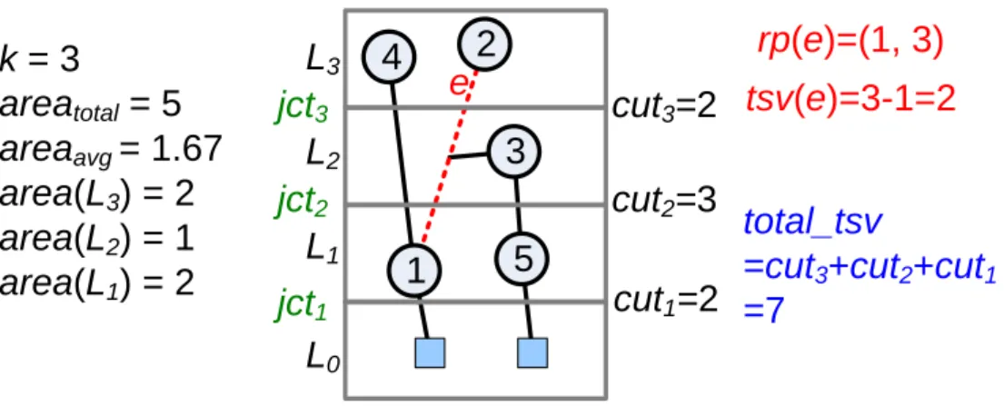
cut = 5 + 9 + 9 + 5 = 28, including 15 iTSVs connecting between operation cells, and 13 TSVs connecting between operation cells and I/O pads. We would like to emphasize again that existing partitioning algorithms usually ignore the I/O pad connection issue, as well as the provided min-cut-based solutions are generally not well optimized (shown later) and always underestimate the real TSV need even excluding TSVs for connecting I/O pads (8 vs. 15 in this case) due to their layer-unawareness. Figure 10 is an example of the model. Assume the area of each vertex is set to 1. The graph is assigned into a 3-layers 3D architecture. As like Figure 10, the area of each layer is shown. For the hyperedge e, the bottom-most vertex {1} is in Layer 1, and the top-most vertex {2} is in Layer 3. Hence, rng(e) is (1, 3), and the tsv(e) can be calculated by 3-1 = 2. Besides, we can calculate the number of hyperedges through each junction, and total_tsv can be figured out by summed them up.
5
1
2
3
L
1L
2L
34
L
0jct
3jct
2jct
1cut
2=3
cut
1=2
cut
3=2
e
rp(e)=(1, 3)
tsv(e)=3-1=2
total_tsv
=cut
3+cut
2+cut
1=7
k = 3
area
total= 5
area
avg= 1.67
area(L
3) = 2
area(L
2) = 1
area(L
1) = 2
Figure 10. An example of the 3D model.
2.2.4 Problem Formulation
In this work, we model the 3D partitioning problem as a layer-aware multi-way partitioning problem. Given a target 3D structure consisting of k layers stacking vertically, a design G, the I/O constraint, and the area constraint
) 1 ( ) ( ) 1 ( r area L area r
areaavg i avg (2.4)
with a balanced ratio r, 0r1, for balancing the area of layers. Our proposed algorithm partitions G into k sub-designs which are explicitly associated to k different vertical layers so that the total number of TSVs is minimized. That is, given G = (V = C ∪ I, E) with layer(v) = 0, v I, our algorithm finds the mapping, 1 layer(v) k, v C, such that
Chapter 3 Proposed Algorithm
In this chapter we present our bottom-up multi-way 3D partitioning algorithm. Section 3.1 explains why we decide to adopt the iterative framework and how the framework carries out the idea of layer-awareness by unbalanced 2-way partitioning method. In Section 3.2, the further improvement by using k-way partitioning engine is described.
3.1 Iterative Unbalanced 2-Way Partitioning Framework
Here we propose our iterative partitioning framework that gradually constructs the solution from the bottom layer all the way to the top. Section 3.1.1 explains how to use unbalanced 2-way partitioning algorithm iteratively to decide the members of each layer. Then Section 3.1.2 proposed the solution to solve the parasitical area problem in this iteratively constructive framework. Finally, Section 3.1.3 describes our iterative layer-aware partitioning algorithm with unbalanced 2-way partitioning engine iLap-2 in detail.
3.1.1 Iterative Procedure
Before describing the procedure step by step, we have to point out an important concept. Because of the 3D architecture, the partitioning result displays with a permutation. From the bottom layer, if the first layer is fixed, the number of cuts between the first layer and those upper layers will not be changed no matter which layer the other vertices will be located. Since there is a naturally fixed layer in the 3D structures, I/O layer, we can construct the result from it. Based on the concept and this initial fixed layer, this procedure can define the solution layer by layer. Following is an example to detail how we use this concept.
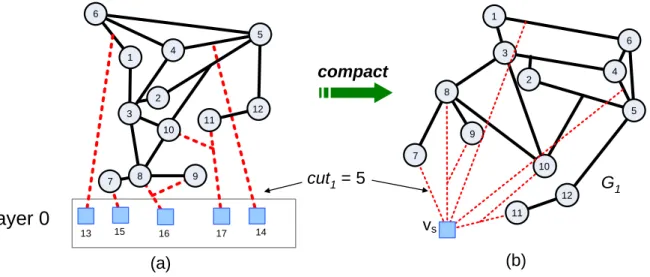
Consider that all I/O pads must reside at L0 by definition and then the number of TSVs through jct1 (i.e., cut1,) is always fixed to |I| no matter how other operation cells (or L1~Lk) get partitioned eventually. Therefore, if we define G1 by compacting all the I/O pads into the
supervertex vs and keeping all the related hyperedges unchanged, as shown in Figure 11, it is conclusive that jct1 will remain unchanged and so will cut1 in G1 if vs is resided at L0.
12 11 10 9 8 7 2 5 1 4 3 6 vs cut1= 5 compact (a) (b) G1 12 11 10 9 8 7 2 5 1 4 3 6 13 15 16 17 14 Layer 0
Figure 11. Compact fixed cells into a supervertex.
ps
1:3
12 11 10 9 8 7 2 5 1 4 3 6 vs G1 12 11 10 9 8 7 2 5 1 4 3 6 vs G1Figure 12. Unbalanced 2-way partitioning.
Next, an arbitrary conventional unbalanced 2-way min-cut partitioner is applied on G1 to get two partitions. Based on the area constraint, the paritioner chooses a part of the operation cells together with vs in the smaller partition ps, where area(vs) is set to zero to avoid disturbing area balancing during partitioning. The partition ps further implies that the operation cells residing in ps should be put as close to the I/O pads as possible for cut minimization and thus should be assigned to L1. For example, Figure 12 indicates the 2-way
min-cut partitioning with an area rate (1:3), and hence L1 is finally set to {7, 11, 12} as Figure 13(a) depicts. cut2= 6 compact G2 (a) (b) 10 9 8 2 5 1 4 3 6 vs 12 11 10 9 8 7 2 5 1 4 3 6 13 15 16 17 14 Layer 1 Layer 0 Figure 13. L1 compaction.
Once the elements of L1 are determined, cut1 is therefore fixed. The next task becomes how to decide which vertices should reside at L2. However, since L0 and L1 are fixed at this point,
jct2 and cut2 are both fixed no matter how other else operation cells (or L2~Lk) get partitioned later. As one can easily discover that the situation is extremely similar as that of identifying L1 previously. Hence, if we further derive G2 from G1 by compacting L1 into vs and apply 2-way min-cut partitioning with the area rate changed into 1:2 on G2, L2 can then be identified in the same fashion (as shown in Figure 14). An important idea is that the partitioning size becomes smaller and smaller.
ps
1:2
10 9 8 2 5 1 4 3 6 vs G2 10 9 8 2 5 1 4 3 6 vs G2 Figure 14. L2 decision.Summarily, at each iteration the proposed framework always derives Gn+1 from Gn by further compacting Ln into vs, then applies unbalanced 2-way min-cut partitioning with variant area rate to get Ln+1. This iterative process is not terminated until Lk–1 is identified. Figure 15 illustrates the final result generated by iLap-2, and the total TSV count is 22.
Layer 1
Layer 0
Layer 2
12 11 10 9 8 7 2 5 1 4 3 6 13 15 16 17 14Layer 3
Layer 4
Cut
4=5
Cut
3=6
Cut
2=6
Cut
1=5
Figure 15. The result of iLap-2.
3.1.2 iLap-2
Before describing the flow of the proposed algorithm iLap-2, two essential terms should be revisited again:
i) The supervertex vs represents a set of vertices, but area(vs) is always set to zero. ii) To compact a vertex v into the supervertex vs is to insert v itself into vs, i.e., vs =
vs∪{v}. Every net originally connected to v is reconnected to vs afterward.
The flow and pseudo code of the complete algorithm are given in Figure 16. All I/O pads are first compacted into the supervertex vs during initialization. Each iteration starts with unbalanced 2-way min-cut partitioning. Once partitioning is done, the vertices residing at the partition where vs also locates are assigned to the current layer, i.e., Layer n. n always increases by one at every iteration end. At the final iteration, where n = k–1, the elements of Layer k–1 are identified after 2-way partitioning. At last, the remaining operation cells are
then automatically assigned to the top-most Layer k and the algorithm ends. That is, exact k–1 invocations of unbalanced 2-way partitioning are needed for k-layer 3D partitioning here.
n < k ? N
Y
End
n←1
Compact I/O into Vs
C←C ∪ {Vs} Unbalanced 2-way partitioning Compact n ← n + 1 Initialization 1 n ← 1;
2 compact all I/O pads into the supervertex vs; 3 C ← C ∪ {vs};
Constructive Loop
4 while(n < k)
5 Unbalanced 2-way min-cut partition(C); 6 foreach vi C– {vs} do 7 If part(vi) == part(vs) do 8 layer(vi) ← n; 9 C ← C– {vi}; 10 compact viinto vs; 11 n ←n + 1; 12 foreach vjC– {vs} do 13 layer(vj) ← k;
Figure 16. The flow and pseudo code of iLap-2.
3.1.3 Parasitical Area Problem
When we use the area constraint defined in Section 2.2 to balance the area of the 3D structures, the partitioning engine allows the clustered area to be minimum and maximum with areaavg(1r) and areaavg(1r) respectively. However, it may produce two kinds
(a) Excess area (b) Insufficient area
Areaavgx (1 - r )
Areaavg x (1 + r )
of area problems on the top-most layer(s). First, if the area of most lower layers is less than
avg
area , the area of top-most layer may be excess like Figure 17(a). On the other hand, if the area of the lower layers is more than areaavg, it is possibly insufficient as shown in Figure 17(b).
To solve these parasitical problems, the additional constraint is added:
k i r L usage area R r i j i i
1 , ) ( _ 1 (3.1) ) ( _usage Liarea : The ratio of the area usage on the i-th layer. It is defined as
avg avg i i area area L area L usage area_ ( ) ( ) .
Ri denotes the summation of the ratio of the area usage from L1 to Li. If we combine equation 2.4 with equation 3.1, the area constraint becomes
) 1 ( ) ( ) 1 ( i,low i avg i,up
avg r area L area r
area , where ) , ( ) , ( 1 , 1 , i up i i low i R r r Min r R r r Min r . (3.2)
That is, different layers have the different balanced ratio numbers, ri,low and ri,up. Depend on the summation of the area usage of previous layers, ri,low and ri,up are the tight boundary calculated by the above equation. Then the balanced ratio numbers are applied into the iterations of the framework. By eq. 3.2, the parasitical area problem will be solved as Figure 18 shows. Assume the balanced ratio r is 5%, L1 is the first layer to reside with r1,up = 5% and
r1,low = 5%. Then, the upper balanced ratio of L2, r2,up, becomes 3% because there is already 2% area usage in L1 (R1=2%). If area_usage(L2) is 2%, R2 is 4%(=area_usage(L1) +
area_usage(L2)). Therefore, r3,up is 1% calculated by Min(r,rR2). Although the area usage
2%
2%
1%
0%
L
1L
2L
3L
4r
1,up=5%
r
1,low=5%
r
2,low=5% r
3,low=5%
r
4,low=5%
r
4,up=0%
r
3,up=1%
r
2,up=3%
R1=2% R2=4% R3=5% R4=0% Area usageAvailable area usage
Figure 18. An example for different area ratio.
3.2 Iterative k-Way Partitioning Framework
For Figure 8(b), the result produced by iLap-2 (Figure 15) is good, but it is not good enough when compared to the best permutation solution as Figure 8(c). In this section, we describe the reason why iLap-2 can not get the solution like Figure 8(e) firstly. And then we propose the new algorithm named iLap-k to improve the performance.
3.2.1 The Reason to Use k-Way Partitioning Engine
iLap-2 uses unbalanced 2-way partitioning algorithm to reside vertices layer by layer.
Nevertheless, considering only one junction at a time may fall into the local minimum. Figure 19 is a 4-layer example which shows why iLap-2 can not always make the right decision for the future.
2
1
4
6
8
9
3
5
7
10
11
12
2 1 4 6 8 9 3 5 7 10 11 12 2 1 4 6 8 9 3 5 7 10 11 12 Cut4=3 Total TSV = 13 Total TSV = 12 Cut = 3 Cut3=5 Cut2=3 Cut1=2 Cut4=3 Cut3=4 Cut2=3 Cut1=2 (a) (b)2
1
4
6
8
9
3
5
7
10
11
12
Figure 19. A 4-layer example for the local decision of iLap-2.
Obviously the cut size of Figure 19(a) is the same with Figure 19(b), but the partitions clustered with different members into Layer 1, {1, 2, 3} and {1, 2, 4} respectively. After putting those cells into Layer 1, the 2-way partitioning results in the second iteration are also different as like L2 of Figure 19. If we construct the structure sequentially, the final result of Figure 19(a) required 13 TSVs; however there is only 12 TSVs needed in Figure 19(b). In this example, the partitioning results clustered previously influence the later solution. Therefore, if we considered only one junction at a time possibly tend to a bad outcome. In order to consider the global distribution, we replace the partitioning engine in iLap-2 by k-way min-cut partitioning.
For instance, Figure 20 is the result associating to Figure 19 partitioned by k-way engine. The chosen part with the supervertex is unchanged. Then the engine partitions the remaining cells into three parts as minimizing the total cut size as possible. Obviously, the total cut in Figure 20(b) is less than in Figure 20(a). Thus, it’s easy for iLap-k to figure out the difference between these two situations. In brief, we use the k-way partitioning algorithm in the
2 1 4 6 8 9 3 5 7 10 11 12 (b) Total cut = 7
2
1
4
6
8
9
3
5
7
10
11
12
(a) Total cut = 8
Figure 20. Different results in k-way partitioning.
(a) (b) 12 11 10 9 8 7 2 5 1 4 3 6 13 15 16 17 12 11 10 9 8 7 2 5 1 4 3 6 14 12 11 10 2 5 1 4 3 6 (c) (d) vs vs 12 11 10 9 8 7 2 5 1 4 3 6 13 15 16 14 17 cut3 = 4 cut2 = 5 cut1 = 5 cut0 = 5 total_tsv = 19 G1 G2
Different from the 2-way partitioning engine, we apply k-way partitioning algorithm considering the total min-cut afterwards. At each iteration, it can generally predict the distribution of the operation cells and choose the best part as the partial solution. Figure 21 is a simple example of iLap-k. Even though the graph is partitioned into four parts in (a), only one part with vs is put into Layer 1 as Figure 21(b). Then G1 becomes G2 by compacting {7, 8, 9} into vs. Figure 21(d) shows the final result with the number of TSVs less than the best permutation in Figure 8(c).
3.2.2 iLap-k
The following is the pseudo code and the algorithm flow of iLap-k. The procedure is similar to iLap-2. Instead of the unbalanced min-cut 2-way partitioning algorithm, multi-way min-cut partitioning engine is applied to reside those operation cells iteratively. From the bottom layer, the n-th iteration performs with (k–n+1)-way min-cut partitioning until Lk-1 and
Lk are assigned.
Initialization
1 n ← 1;
2 compact all I/O pads into the supervertex vs; 3 C ← C ∪ {vs};
Constructive Loop
4 while(n < k)
5 (k-n+1)-way min-cut partition(C); 6 foreach viC– {vs} do 7 If part(vi) == part(vs) do 8 layer(vi) ← n; 9 C ← C– {vi}; 10 compact viinto vs; 11 n ←n + 1; 12 foreach vjC– {vs} do 13 layer(vj) ← k; n < k ? N Y End n←1
Compact I/O into Vs
C←C ∪ {Vs}
(k-n+1)-way partitioning
Compact
n ← n + 1
In summary, the proposed framework possesses following four unique features:
i) It invokes multi-way min-cut partitioning at every iteration. The major reason is to find the set of operation cells closest to the previous junctions, which potentially minimizes the TSVs of the current junction. However, since only one partition is actually accepted at each iteration, then why balanced multi-way instead of unbalanced two-way? The main reason is to better mimic the final solution, which potentially produces a more stable outcome.
ii) Once a junction (and thus a cut) is fixed in an iteration, it is never altered during following iterations. This ensures that good decisions made previously are never overthrown later.
iii) At each iteration, only one partition is accepted and decisions for other partitions are actually discarded. Later the updated graph topology is reexamined and better decisions are dynamically remade at the following iteration. For instance, L2 = {1, 3, 10} in Figure 21(d) is not identical to any partition shown in Figure 21(a). Running any of conventional multi-way min-cut partitioning algorithms just once simply cannot get this kind of result.
iv) From the traditional partitioning perspective, the result in Figure 8(d) has a larger total cut size than the result in Figure 8(a) (10 vs. 8). However, we already show that the former one results in a better 3D partitioning solution. It is clear that the total cut size, which is layer-unaware, is not an appropriate metric in 3D partitioning. Again, this is the other evidence that conventional multi-way min-cut partitioning algorithms hardly compete with the proposed iterative framework.
In this thesis, we adopt the well-known hMetis as the internal partitioning engine. However, our proposed framework can obviously co-work with any multi-way min-cut partitioning engines. It implies that a better engine (if any) may be adopted for better 3D partitioning results in the future.
Chapter 4 Experiments
After introducing the main idea of iLap in the previous chapter, the distribution of TSVs is analyzed in this chapter. iLap always wins on the number of TSVs no matter the number of layers increases. In this chapter, the result how much iLap outperforms the other algorithms is presented.
4.1 Environment Setup
iLap has been implemented in C++/Linux environment. We demonstrate the effectiveness
of iLap through a series of comparisons with three hMetis-based methods and multilevel multilayer partitioning algorithm as showing in Figure 23:
Layer-aware
Layer-aware
3D partitioning
3D partitioning
Layer-unaware
Layer-unaware
hMetis
hMetis
EX-hMetis
EX-hMetis
EV-Matrix
EV-Matrix
Iterative
Iterative
Multilevel
k-layer partition
(MKLP)
Multilevel
k-layer partition
(MKLP)
Non-iterative
Non-iterative
iLap-k
iLap-k
iLap-2
iLap-2
Figure 23. Classification of 3D partitioning.
i) hMetis: It applies hMetis to produce the min-cut partitions, and then those parts
area layered according to their original sequential tags (i.e., in random order) [27].
ii) EX-hMetis: It applies hMetis to produce the min-cut partitions, and then those parts are best layered through exhaustively examining all possible layer permutations.
iii) EV-matrix: It applies hMetis to produce the min-cut partitions, and then those parts are layered by the method described in [22].
iv) MKLP: It is the multilevel multilayer partitioning algorithm proposed in [19]. Notice that the three hMetis-based methods all start with the same set of partitions and their final result variances solely come from different layer assignments. We evaluate the performance of iLap (iLap-2 and iLap-k) and other four methods over a set of 14 test cases consisting of 10 cases from the MCNC benchmark set [30], three large cases (cfft, aqua, and
video) from Altera [31], and one 128-point FFT design (fft128) [32]. The area cost of every
operation cell can be any number, in order to be calculated easily, each area cost is uniformly set to one in our experiments. In addition, the setting of the balanced ratio is 0.05 as like other works. We perform ten experimental runs on every test case with different random seeds and find the average as the result. All experiments are conducted on a workstation with an Intel Xeon 2GHz CPU and 14GB RAM.
4.2 Results and Analyses
4.2.1 Analysis of TSV Count with Fixed Layer
Table 2 reports the TSV demands as the number of layers in a 3D IC is set to 4. It seems
EV-matrix just performs equally well as plain hMetis. Meanwhile, given a set of 4 partitions
generated by hMetis, EX-hMetis always picks the one with the lowest TSV count out of 4! = 24 different permutations (i.e., layer assignments) and consequently EX-hMetis on average attains 16% TSV reduction as compared with hMetis. Furthermore, MKLP shows its layer-aware advantage on the three largest cases about 70% reduction. Nevertheless, it’s not reliable in others. For iLap-2, it performs as well as EX-hMetis on average. Besides, it is more efficient than EX-hMetis in the larger cases. Due to considering the overall situation and predicting the distribution in the future during the framework, iLap-k improves iLap-2 about 19% on average and reduces TSV count by 36% and 24% as compared to hMetis and
EX-hMetis, respectively. Moreover, for the largest three test cases (cfft, aqua, and video), iLap-k even outperforms hMetis by more than 75%. Though hMetis is an excellent multi-way
min-cut partitioning algorithm, it fails to be a good 3D partitioner due to its layer-unawareness. Even EX-hMetis with exhaustive permutations still cannot defeat iLap-k. Compared with MKLP, iLap framework dynamically and iteratively selects the partial best to construct the better result. Therefore, it concludes that a dedicated layer-aware 3D partitioning algorithm, like iLap, should be regarded as one of the essential components while constructing a sophisticated 3D IC design environment.
Table 2. Total number of TSVs when k = 4.
If we experience in 8 layers as Table 3 shows, EV-Matrix cannot always improve the result of hMetis since it weakly solves the hyperedge problem. In hMetis-based algorithms,
EX-hMetis is also the best solution. For MKLP, it can not find a good solution when the small
circuits are partitioned into high number of layers. However, it does well on the largest three cases. Compared with other methods, iLap-2 and iLap-k are still demanded the least number of TSVs.
4.2.2 TSV Count
Figure 24 depicts the average TSV count over 14 test cases as a function of the number of layers; and three points are worth pointing out. Firstly, the more layers a design gets partitioned into, the more TSVs it generally requires. Secondly, iLap-k and iLap-2 are the all-time winner from 2 layers to 10 layers among all methods. Thirdly, unlike the layer-unaware methods, the number of TSVs required by layer-aware algorithms raises very smoothly as the number of layers increases.
Taking hMetis as the baseline, Figure 25 reveals the average TSV ratios over the number of layers; and three points are worth pointing out here. Firstly, iLap-k constantly and steadily outperforms hMetis by about 33% in TSV size regardless of the number of layers. Secondly, from the curve we can see that iLap-2 is nearly equal to EX-hMetis. Finally, EX-hMetis is always outperforms hMetis, as expected.
Figure 25. Normalized TSV count.
4.2.3 Distribution of TSV Count
Meanwhile, Figure 26 presents the average standard deviations of TSV count over a different number of layers. It is evident that the standard deviation of TSV count associated with iLap-k and iLap-2 are more stable than the others. As previously mentioned, a TSV occupies significant silicon estate so that high standard deviation of TSV count potentially worsens area size imbalance among individual layers and even lowers the yield of a design.
Figure 27 reports the average maximum TSV count at some junction of a design over a different number of layers; and iLap-k and iLap-2 always possess the lowest values regardless of the number of layers. For some 3D logic structures, like 3D FPGAs, the number of pre-fabricated inter-layer TSVs is fixed. Hence the design mapping is considered a failure even if the required TSVs exceeds the provided ones only at one junction, and a high maximum TSV count potentially increases such chances.
Figure 26. Standard deviation of TSV count.
4.2.4 Runtimes
Regarding the runtime efficiency issue, Figure 28 gives the average runtime of 14 test cases in second over a different number of layers. It is evident that both hMetis and EV-matrix are very time-efficient. The runtime required by iLap-k and iLap-2 grow linearly as the number of layers increases. This trend is natural since the number of invocations for multi-way partitioning inside iLap-based algorithms also grow linearly as the number of layers increases. Since the iterative engine in iLap-2 is a simple 2-way partitioning, it is faster than MKLP when the number of layers increases. Even the engine in iLap-k is more complex, only a few seconds needed to complete the algorithm. Hence, given the excellent performance in TSV minimization, the time complexity of iLap-k should be acceptable. As for EX-hMetis, since it has to check all possible permutations to find the best one, the required runtime is thus exponential to the number of layers. It is no wonder why the runtime increases drastically as the number of layers exceeds 8. Even though using some skills to improve the runtime of
EX-hMetis, it still cannot improve the quality.
Chapter 5 Conclusion
Using TSVs as the vertical links is a famous technology in 3D structure. However, the area overhead and the reliability of TSVs become a big problem seriously. Therefore, in this thesis we present two iterative layer-aware partitioning algorithms, iLap-2 and iLap-k, for minimizing the total number of TSVs in 3D ICs. They utilize the unbalanced two-way min-cut partitioning and the multi-way min-cut partitioning engine inside the iterative frameworks respectively to gradually construct the final results layer by layer in the bottom-up fashion. Besides, the parasitical area problems in this kind of iterative methods are solved by the additional area constraint we proposed. The experimental results clearly demonstrate that iLap-2 reduces the TSV count as good as EX-hMetis in a few seconds. In addition, iLap-k, which enhances the efficiency of iLap-2, is capable of reducing the total TSV count by about 33% compared to layer-unaware hMetis. Moreover, both of iLap-k and
iLap-2 experience a smooth TSV increase as the number of layers raises, and distribute TSVs
more evenly among different vertical layers preventing any layer junction from having a burst number of TSVs. Although they need more iterations to construct the result, they only demand an acceptable runtime. Consequently, compared to the existing methods, we believe
iLap is a better alternative for design partitioning in state-of-the-art 3D IC design
References
[1] International Technology Roadmap for Semiconductor. Semiconductor Industry Association, 2005 – 2009.
[2] G. Metze, M. Khbels, N. Goldsman, and B. Jacob, “Heterogeneous integration,” Tech Trend Notes, vol. 12, no. 2, pp. 3, 2003.
[3] R. R. Tummala and V. K. Madisetti, “System on chip or system on package?” IEEE Design & Test of Computers, pp. 48 – 56, Apr. – Jun., 1999.
[4] P. H. Shiu and K. S. Lim, “Multi-layer floorplanning for reliable system-on-package,” Proc. of the 2004 International Symp. on Circuits and System, pp. 23 – 26, May 2004. [5] K. L. Tai, “System-in-package (SIP): challenges and opportunities,” Proc. of Asia and
South Pacific Design Automation Conference, pp. 191 – 196, 2000.
[6] S. Spiesshoefer et al. “Process integration for through-silicon vias,” Journal of Vacuum Science and Technology A, vol. 23, no. 4, pp. 824 – 829, Jul. 2005.
[7] K. Banerjee, S. J. Souri, P. Kapur, and K. C. Saraswat, “3-D ICs: a novel chip design for improving deep submicron interconnect performance and systems-on-chip integration,” Proc. IEEE, vol. 89, pp. 602 – 633, 2001.
[8] A. W. Topol et al. “Three-dimensional integrated circuits,” IBM Journal of Research and Development, vol. 50, no. 4/5, pp. 491 – 506, July/September 2006.
[9] G. Philip, B. Christopher, and P. Ramm, “Handbook of 3D integration,” Wiley-VCH, 2008.
[10] C. Ferri, S. Reda, and R. I. Bahar, “Parametric yield management for 3D ICs: models and strategies for improvement,” Journal Emerging Technologies in Computing Systems, vol. 4, no. 4, Article ID 19, Oct. 2008.
[11] I. Loi et al. “A low-overhead fault tolerance scheme for TSV-based 3D network on chip links,” Proc. International Conference on Computer-Aided Design, pp. 598 – 602, 2008. [12] Sung Kyu Lim, “TSV-aware 3D physical design tool needs for faster mainstream
acceptance of 3D ICs,” ACM DAC Knowledge Center (dac.com), 2010.
[13] D. H. Kim, K. Athikulwongse, and S. K. Lim, “A study of through-silicon-via impact on the 3D stacked IC layout,” Proc. International Conference on Computer-Aided Design, pp. 674 – 680, 2009.
[14] E. Beyne et al. “Through-silicon via and die stacking technologies for microsystems-integration,” Proc. IEEE International Electron Devices Meeting, 2008.
[15] J. Cong and G. Luo, “A multilevel analytical placement for 3D ICs,” Proc. of Asia and South Pacific Design Automation Conference, pp. 361 – 366, 2009.
[16] J. Cong, G. Luo, J. Wei, and Y. Zhang, “Thermal-aware 3D IC placement via transformation,” Proc. of Asia and South Pacific Design Automation Conference, pp. 780 – 785, 2007.
[17] B. Goplen and S. Spatnekar, “Placement of 3D ICs with thermal and interlayer via considerations,” Proc. Design Automation Conference, pp. 626 – 631, 2007.
[18] I. H.-R. Jiang, “Generic integer linear programming formulation for 3D IC partitioning,” 22nd IEEE International SOC Conference, 2009.
[19] Y. L. Chung, Y. C. Hu, and M. C. Chi, “A multilevel multilayer partitioning algorithm for three dimensional integrated circuits,” International Symposium on Quality Electronic Design, pp. 483 – 487, 2010.
[20] G.-Y. Pan and et al. “An iterative partition algorithm to minimize area and vertical interconnections for three-dimensional integrated circuits,” Proc. 20th VLSI Design/CAD Symposium, 2009.
[21] C. M. Fiduccia and R. M. Mattheyses, “A linear time heuristic for improving network partitions,” Proc. Design Automation Conference, pp.175 – 181, 1982.
[22] C. Ababei and K. Bazargan, “Non-contiguous linear placement for reconfigurable fabrics,” Proc. Reconfigurable Architectures Workshop, pp. 141 – 148, 2004.
[23] C. Ababei, H. Mogal, and K. Bazargan, “Three-dimensional place and route for FPGAs,” Transactions on Computer-Aided Design of Integrated Circuits and Systems, vol. 25, no. 6, pp. 1132 – 1140, Jun. 2006.
[24] http://mountains.ece.umn.edu/~kia/Download/tpr.html
[25] K. Siozios, A. Bartzas, and D. Soudirs, “Architecture-level exploration of alternative interconnection schemes targeting to 3D FPGAs: a software-supported methodology,” International Journal of Reconfigurable Computing, vol. 2008, Article ID 764942, 2008. [26] K. Siozios, V. F. Pavlidis, and D. Soudirs, “A Software-Supported Methodology for
Exploring Interconnection Architectures Targeting 3-D FPGAs,” Design, Automation and Test in Europe Conference & Exhibition, 2009.
[27] G. Karypis, R. Aggarwal, V. Kumar, and S. Shekhar, “Multilevel hypergraph partitioning: applications in VLSI domain,” Transactions on VLSI Systems, vol. 7, no. 1, pp. 69 – 79, Mar. 1999.
[28] http://glaros.dtc.umn.edu/
[30] S. Yang, “Logic synthesis and optimization benchmarks user guide,” Technical Report 1991-IWLS-UG-Saeyang, Microelectronics Center of North Carolina, 1991.
[31] http://www.eecs.berkeley.edu/~alanmi/benchmarks/altera/old/altera12_blif_baf.zip. [32] T. H. Cormen, C. E. Leiserson, R. L. Rivest, and C. Stein, Introduction to Algorithms,
![Figure 1. Relative delay vs. process technology. [1]](https://thumb-ap.123doks.com/thumbv2/9libinfo/7645046.138694/11.892.193.754.530.1051/figure-relative-delay-vs-process-technology.webp)