Chin-Teng Lin, Li-Wei Ko, and
Tzu-Kuei Shen
Digital Object Identifier 10.1109/MCI.2009.934559
Abstract: Driving is one of the most common attention-demanding tasks
in daily life. Driver’s fatigue, drowsiness, inattention, and distraction are reported a major causal factor in many traffic accidents. Due to the drivers lost their attention, they had markedly reduced the perception, recognition and vehicle control abilities. In recent years, many computational intelligent technolo-gies were developed for preventing traffic accidents caused by driver’s inattention. Driver’s drowsiness and distraction related studies had become a major interest research topic in automotive safety engineering. Many researches had investigated the driving cog-nition in cognitive neuro-engineering, but how to utilize the main findings of driving-related cognitive researches in traditional cognitive neuroscience and integrate with computational intel-ligence technologies for augmenting driving performance will become a big challenge in the inter-disciplinary research area. For this reason, we attempt to integrate the driving cognition for real life application in this study. The implications of the driving cognition in cognitive neuroscience and compu-tational intelligence for daily applications are also demonstrated through two common attention-related driving studies: (1) cognitive-state monitoring of the driver performing the realistic long-term driving tasks in a simulated realistic-driving environment; and (2) to extract the brain dynamic changes of driver’s distraction effect during dual-task driving. Experimental results of these studies provide new insights into the understanding of complex brain functions of participants actively performing ordinary tasks in natural body positions and situations within real operational environments.
1. Introduction
D
riving is one of the most common attention-de-manding tasks in daily life. Driver’s fatigue, drowsi-ness, inattention, and distraction are reported a major causal factor in many traffic accidents. Due to the drivers lost their attention, they had markedly reduced the perception, recognition and vehicle control abilities. In recent years, many computational intelligent technologies were developed for preventing traffic accidents caused by losing driver’s attention. Driver’s drowsiness and distraction related studies had become a major interest research topic in auto-motive safety engineering. Physiological changes such as eye activity measures, heart rate variability (HRV) and particularly electroencephalogram (EEG) activities are known to be asso-ciated with these cognitive changes. In the past, there are many driving-related studies which had investigated the driv-ing performance in human factors or in cognitive neurosci-ence. Recently, some studies had attempted to apply computational intelligence to estimate driver’s cognitive state, but there are still fewer studies to investigate driving cogni-tion and its applicacogni-tion at the same time. Consequently, how to utilize the main findings of driving-related cognitive researches in traditional cognitive neuroscience and integrate with computational intelligence technologies for augmenting driving performance will become a big challenge in the inter-disciplinary research area between cognitive neuroscience and computational intelligence.For this reason, we attempt to integrate the driving cog-nition for real life application in this study. In the begin-ning, we had constructed the simulated realistic-driving environment for the volunteer subjects performing driving-related cognitive experiments. We then measure driver’s physiological signals in this environment and study their fundamental physiological changes in the performing driv-ing tasks. The only possible physiological modality fulfilldriv-ing
the measurement limitation in real-life application is elec-troencephalography (EEG). EEG is a powerful non-invasive tool widely used for both medical diagnosis and neurobio-logical research because it can provide high temporal reso-lution in milliseconds which directly reflects the dynamics of the generating cell assemblies. EEG is also the only brain imaging modality that can be performed without fixing the head/body. After understanding the brain dynamic changes on driving cognition, we then develop some computational intelligence technologies based on these physiological phe-nomena to investigate brain computer interaction.
For any application involving EEG one of the essential and important steps is to remove artifacts due factors such as eye-blinking, muscle noise, and heart signals. One of the commonly used techniques for cleaning of such noises is Independent Component analysis (ICA). However, neuro-scientists usually select the useful independent components manually by looking at the scalp-plot. Consequently such approaches are not useful for real-time such as drowsiness detection in drivers, games based on brain computer inter-face (BCI). Hence, we propose a family of algorithms based on neural networks and support vector machines for automatic identification of useful independent compo-nents. The utility of the proposed approaches is demon-strated using 10-fold cross validation. We have also used fusion methods to improve the detection accuracy further. We have found that when we use a majority voting princi-ple it is not necessarily true that higher vote corresponds to better decisions. This counterintuitive behavior may be because of the subjective variability in the EEG data. This study also suggests that it is possible to developing a “uni-versal” machine for artifact removal in EEG. At last, the implications of the driving cognition in cognitive neuro-science and computational intelligence for daily applica-tions are also demonstrated through two common attention-related driving studies: (1) cognitive-state moni-toring of the driver performing the realistic long-term driving tasks in a simulated realistic-driving environment; and (2) to extract the brain dynamic changes of driver’s distraction effect during dual-task driving. The experimen-tal results of these studies provide new insights into the understanding of complex brain functions of participants actively performing ordinary tasks in natural body posi-tions and situaposi-tions within real operational environments. 2. Materials and Methods
This study would investigate how to augment driving perfor-mance due to driver’s fatigue and attention have been implicated as the causal factors in many accidents. The development of
human cognitive state monitoring system for the drivers to prevent accidents behind the steering wheel has become a major focus in the field of safety driving. Hence, we in public call for volunteer subjects to perform the driving-related cognitive exper-iments and simultaneously measure their physiological signals and mental information in the constructed simulated realistic-driving environment for the realistic-driving safety issue. In the follow-ing sections, we will briefly introduce the physiological signals recording equipment, signal preprocessing and the experimen-tal environment.
2.1 Physiological Data Acquisition
In this study, all volunteer subjects performed the driving-related cognitive experiments until reaching the satisfactory perfor-mance after the placement of the EEG cap and electrodes. During the experiments, subjects were instructed to continu-ously perform the tasks as best as they could. No intervention was made when the subjects was occasionally fell asleep and stopped responding. After such non-responsive periods subjects resumed task performance without experimenter intervention. The onset of each deviation and the subject’s reaction time were recorded at the rate of 60 Hz via a synchronous pulse marker train that was recorded in parallel by the EEG acquisi-tion system for the further off-line analysis. Each subject at least had to complete one 60-minute session in all driving-related cognitive experiments in this study.
Subjects were with a movement-proof electrode cap with 32 sintered Ag/AgCl electrodes for measuring the electrical activates of the brain and that is the electroencephalogram (EEG). Electrodes were placed according to the standard international 10–20 system. Active sites were referenced to linked left and right mastoids. EEG signals were recorded and amplified by the Scan NuAmps Express system (Compumed-ics Ltd., VIC, Australia) with a sampling rate at 250 Hz and 16-bit precision. All channels were referenced to the right mastoid with input impedance lower than 5 kV. At the end of each completely session, the location of the electrodes were digitized with the 3D digitizer (Polhemus 3 space eastrak). The recorded EEG data were preprocessed using a simple low-pass filter and a high-pass filter with cut-off frequency above 50 Hz and below 0.5 Hz, respectively, to remove 60 Hz line noise, high-frequency artifacts and electro-galvanic signals before further analysis. Then these preprocessed EEG signals were fed to independent component analysis (ICA) to decompose EEG signals into various temporally statistical independent activations.
2.2 Independent Component Analysis
Independent component analysis (ICA) [1–3] is a signal pro-cessing technique and uses a measure of statistical indepen-dence to separate mixed signals that are generated by distinct sources but are recorded as a linearly mixed signal. ICA finds the signal components that are maximally independent.
ICA is used to separate mixed signals composed of
several distinct sources (such as EEG) in which the
signal components are maximally independent.
Hence, it can be used to denoise EEG signal when it is mixed with different artifacts such as blinking of eyes. Let
X 1t2 5 1x11t2, x21t2, c, xn1t2 2T be an n-dimensional data vector observed at time
t and S1t2 5 1s11t2, s21t2, c, sn1t2 2Tbe the
vector of independent source signals. The
ICA assumes a data model X1t2 5 AS1t2, where A is an
n 3 n mixing matrix. The ICA finds the A and hence when
A has full rank then using A-1 we can find the unmixed (or
independent) source signals. The ICA algorithm makes an assumption the aggregation of signals from different EEG sources is linear and instantaneous (no time delay). In gener-al, for given data set X, an ICA algorithm produces both A and S. The EEGLAB [4] provides a tool for the visualization of a column of A21, which is known as the component scalp map. Therefore, the independent components are generated using the EEGLAB developed in MATLAB (The Math Works, R2007a).
The ICA methods were extensively applied to blind source separation problem since 1990s [5–8]. Subsequent technical reports [9–12] demonstrated that ICA was a suitable solution to the problem of EEG source segregation, identification, and localization. In this study, we used an extended version of infor-max algorithm of Bell and Sejnowski [2] that can separate sources with either super- or sub-Gaussian distributions, to decompose distinct brain activities. It has also been used in our previous studies [19–21].
2.3 Experimental and Simulated Realistic-Driving Environment
Most driving-related cognitive experiments were adopted to measure the physiological or psychophysical responses while participants performed a computer-simulated driving task in a well-controlled laboratory in which driving controls were a joystick or a steering wheel in front of a computer screen. In such studies, behavioral data such as reaction time to perform sudden braking or turning maneuvers are often measured. However, participants are never provided with kinesthetic input or sensation during these experiments. The lack of multi-sensory (visual, auditory, kinesthetic and tactile) infor-mation presented to participants limits the assessment and interpretation of the complicated relationships between such information and the motor actions of the participants. The ideal experimental condition would
measure physiological signals in an actual automobile on the road. However, inves-tigating driving perception in an actual driving environment would be subject to several limitations. First, ethical con-cerns would prohibit exposing subjects to physical danger of attention lapse while driving an automobile. Second, appropriate data acquisition and moni-toring devices are needed to study the
rapid physiological responses of kinesthetic stimuli. Simulators provide simple and repeatable stimulation to control the parameters of the experiment. Third, objective evaluation of driving performance and putative level of alertness may be dif-ficult to assess on the road.
To overcome such limitation of investigating kinesthetic perceptions during driving, a realistic simulator is the best alternative for driving-related research [13–16]. Hence, we had established an experimental and simulated realistic-driving environment as a test platform for studying the EEG dynamics [16–23] associated with cognitive-state changes during driving in this study. Our past study [22] also demonstrated the differ-ence of brain dynamics with and without kinesthetic stimuli and sensation in the simulated realistic-driving environment. The environment can provide visual, auditory and, most importantly, kinesthetic and tactile stimulation either separate-ly or jointseparate-ly to volunteer subjects, which are not available in conventional EEG laboratories. This dynamic driving simula-tor enables systematic testing of the limitations of normal human performance in sustained-attention tasks in a safe yet realistic environment.
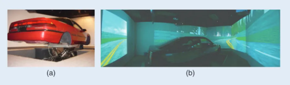
This environment is consisted of an actual automobile mounted on a 6-degree-of-freedom (DOF) Stewart platform (Figure 1(a)) and 3608 surrounded virtual-reality (VR) based driving scenes projected by seven projectors (Figure 1(b)). The 6-DOF motion platform is controlled by six hydraulic linear actuators to generate translational and rotational movement as well as vibratory feedback to simulate actual driving conditions. The 3608 projection of driving scenery is updated synchro-nously with deviations caused by wheel/paddle movement by the subjects or by road conditions such that subjects feel the car moving as if they are driving in real-world conditions. The motion platform also provides physiological and behavioral response recordings to not only to evaluate driving perfor-mance and behavior but also to examine the brain dynamics in response to the kinesthetic stimulation generated by the motion platform. Therefore, this test environment provides an
(a) (b)
FIGURE 1 (a) The driving cabin simulator mounted on a 6-DOF dynamic Stewart motion platform. (b) The simulated realistic-driving environment.
To overcome such limitation of investigating
kinesthetic perceptions during driving, a simulated
realistic driving environment is the best alternative for
driving cognition research.
interactive, safe and realistic environment at very low cost, and the outcomes of this study should be highly applicable to real-life driving safety research.
3. An Automatic Classification System for Useful Brain Sources Selection
For any application involving EEG signals, one of the essential and important steps is to remove artifacts such as eye-blinking, muscle noise, and heart signals. One of the commonly used tech-niques for cleaning of such noises is ICA which is briefly described in the above section. However, some neuroscientists and psychologists usually select the useful independent compo-nents, called useful brain sources, manually by looking at the scalp-plot. Consequently such approaches are not useful for real-time applications such as drowsiness detection in drivers, games based on brain computer interface (BCI). Here in this section, we propose a family of algorithms based on neural networks and support vector machines for automatic identification of useful independent components. The utility of the proposed approaches is demonstrated using 10-fold cross validation. We have also used fusion methods to improve the detection accuracy further. Based on the experimental results, we found that when we use a major-ity voting principle, it was not necessarily true that higher vote corresponded to better decisions. This counterintuitive behavior might be because of the subjective variability in the EEG data. This study also suggests that it is possible to develop a “universal” machine for artifact removal in EEG.
Among the different methods of artifacts removal, ICA, [24] is a frequently used method. ICA methods generally assume that the signals recorded on the scalp are mixtures of time courses of temporally independent cerebral and non-cerebral sources. The potentials generated by different parts of the brain, scalp, and body are linearly summed at the recording electrodes. ICA also assumes that the propagation delays are not significant. Many investigations have demonstrated that ICA could separate the artifacts and raw EEG signals [24–31]. Jung et al. in [31] proposed a method for isolating and removing different types of EEG arti-facts by linear decomposition using an extension of the Bell & Sejnowski,’s information-maximization ICA algorithm [2–3]. The extended algorithm [3] can separate sources with either super-Gaussian or sub-Gaussian amplitude distributions. This enables one to remove line noises efficiently. The algorithm does not require reference channels for the artifact sources. The meth-od first finds the independent time courses of different cerebral and artifact sources and then the cleaned EEG signals are obtained by eliminating the contributions of the artifact sources.
Authors in [27–30] have used ICA to remove the effect of eye-blinking. Electrooculography (EOG) signals can be used to record the artifacts caused by eye-blinking in EEG signal. Then
a linear combination of EOG signal recorded at different sampling time can be subtracted to find the artifact free EEG. Also, the EOG signal can be compared with the independent components to identify independent compo-nents relating to EOG related artifacts [30]. Researchers have investigated the problem of removing the effect of eye-blinking removal for a long time. Among various approaches such as Average Artifact Subtraction (AAS) [32] and Principle Component Analysis (PCA) [31], ICA is found to do a better job of removing artifacts. The AAS method finds similar artifact peaks and averages these artifacts to generate a subtrac-tion model. This is then subtracted from the noisy EEG to get the clean EEG signals [33–34]. But this method does not rule out the possibility of including some useful actual EEG signal in the subtraction model, and hence it may induce distortions on scalp maps. The PCA method translates the original data into some important components, which could preserve most vari-ability of the original signal in a lower dimension. PCA based methods result in components where a single component may contain too much information (signal). The artifact components extracted from ICA are generally found to exhibit stronger cor-relation with the actual artifacts than that by the PCA artifact components [31]. Furthermore, because PCA usually mixes the EEG and artifacts, if a component is removed, the cleaned EEG signal may contain less EEG signal for the analysis. Moreover, McKeown et al. [35] made an interesting comparison between PCA and ICA which had shown that ICA performed better. All these have motivated us to consider ICA based artifact removal from EEG signals. For these reasons, we chose the ICA method to remove the artifacts.
This study attempts to demonstrate that it is feasible to develop such a “universal” machine. Here, we use four machine learning tools, the usual multilayer perceptron (MLP) architec-ture with hyperbolic tangent signal function (MLPTAN) and MLP architecture with redial basis function signal function (MLPRBF), the radial basis function neural network (RBFNN), and the support vector machine with radial basis kernel func-tion (SVMRBF). Some experimental results have been report-ed in references [36–37]. To demonstrate the performance of proposed automatic component selection system, we use a 10-fold cross validation protocol to check the consistency of training data which are collected by 25 volunteer subjects, and apply to the testing data from other 10 volunteer subjects to evaluate the classification accuracy.
3.1 Experimental Data Collection and Feature Extraction For this study, we have generated the EEG data using a simulat-ed realistic-driving environment [16–23] establishsimulat-ed in the Brain Research Center of the National Chiao Tung University. The EEG data are collected when each subject performs an hour long-term driving task, which is subjected to the experi-mental driving-related cognitive tasks. Each subject is instructed to respond to the experimental tasks and maintain a good driving performance on the road. As shown in this study, these
ICA are widely used to remove the artifact EEG signals
such as eye-blinking, muscle noise, and heart signals in
many biomedical researches.
driving-related cognitive tasks are like drowsiness, distraction and motion sickness driving. In this study, although we used 32-ch international 10–20 system for EEG signal recording, we will get 28 channels EEG signals except four channels such as the
reference, ground, FP1 and FP2 channels. The electrode loca-tions of FP1 and FP2 are closed to eye movement which will easily affect clean EEG signals. Hence, we ignore the recording signals from these areas. In the experiments, we have used 35 volunteer subjects. Of these 35, data on 25 subjects were col-lected earlier and develop a global automatic scheme for useful independent components selection from
these 25 subjects, called training data. For the evaluation performance of this auto-matic scheme, we used other EEG data-sets acquired from another 10 subjects as the testing data.
For each subject, we have 28 indepen-dent components extracted by 28 EEG channels and hence 28 scale-maps(SM),
SM1, SM2 . . . and SM28. We use some well experienced neuroscientists who can interpret/analyze EEG to label each scalp map as signal (useful com-ponent with label 1) or as artifact (not useful with label 0). Figure 2 displays the 28 scalp maps extracted by a single subject. In Fig. 2, we have labeled the useful components as good and the remaining ones as bad. For example, the 1st, 6th and 18th components are labeled as bad as these possibly corre-spond to eye blinking. We emphasize that there may be some scalp-maps on which the well experienced neu-roscientists may not agree about clas-sifying the maps as artifacts or not.
In this study, we use totally 980 weighting vectors from different 35 subjects including training and testing data, each vector representing a corresponding independent component.
3.2 The Automatic Classification System
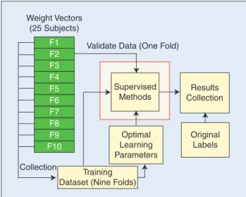
As mentioned in above, we developed an automatic compo-nent classification system in this study. To demonstrate the per-formance of the proposed system, we use a 10-fold cross validation protocol to check the consistency of training data and apply to the testing data to evaluate the classification accu-racy. Figure 3 is showing the 10-fold cross-validation of train-ing algorithm structure. In this study, the traintrain-ing data collected from 25 subjects which can totally generate 700 training com-ponents. These ICA components are partitioned randomly into 10 folds with equal size. We leave one of the 10 folds out for validation performance and the reaming 9 folds are used to
train an automatic scheme for useful component selection. In the kernel of supervised training method, we use the support vector machine with RBF kernel (SVMRBF) and three types of neural network (MLPTAN, MLPRBF and RBFNN) to develop the automatic component selection. The RBF and MLP networks are the two most widely used neural networks for
C1 Bad C2 Good C3 Good C4 Bad C5 Good C6 Bad
C7 Good C8 Good C9 Good C10 Good C11 Good C12 Bad
C13 Good C14 Good C15 Good C16 Good C17 Bad C18 Bad
C19 Good C20 Bad C21 Good C22 Bad C23 Bad C24 Bad
C25 Bad C26 Bad C27 Bad C28 Bad
FIGURE 2 A set of illustrative ICA scalp component map labeled by well experienced neuroscientists.
F1
Weight Vectors (25 Subjects)
Validate Data (One Fold)
Supervised Methods Optimal Learning Parameters Collection Training Dataset (Nine Folds)
Results Collection Original Labels F2 F3 F4 F5 F6 F7 F8 F9 F10
FIGURE 3 Ten-fold cross-validation of training algorithm structure.
It is feasible to apply computational intelligence
to develop a “universal” machine for artifact removal
in EEG signals.
pattern recognition application [38]. We have used the back-propagation algorithm for training MLP networks with single hidden layer. The MLPTAN and MLPRBF both are multilayer perceptron networks. Both of them use the log-sigmoid transfer function at the output layer. The only difference between the two networks is in the signal function of the hidden layer. The MLPTAN uses hyperbolic tangent signal function while the MLPRBF uses the radial basis function.
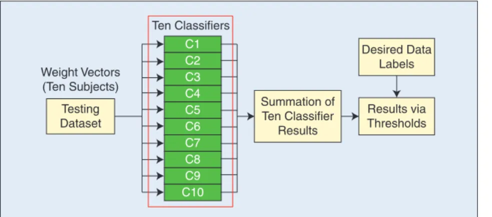
Figure 4 shows the testing algorithm through ten-fold cross validation training classifiers. To evaluate the training algorithm performance, another 10 subjects EEG datasets were applied ICA to extract the testing components. Each subject
also has 28 components in each session. Then we fill the 28 components from each subject to the 10 classifiers which is constructed by 10-fold cross valida-tion of the training algorithm. In this way, we get 10 different classifiers
Ck, k5 1, c, 10. Each of these classi-fiers is designed based on the training data from the 25 subjects. Now each of these 10 classifiers is tested on the testing data obtained from the 10 new subjects. Each classifier generates a value 0 or 1. However, we use the majority vote from the results of these ten classifiers to make the decision but it may be not necessari-ly correct. It might be better to use a threshold to help making the decision. A decision with a higher threshold usually will indicate more confidence on the decision.
3.3 Experimental Results and Discussion
In cross validation results of training data, Table 1 reports the average accuracy and standard deviation through four different machine learning models. We can clearly find that the SVMRBF performs the best accuracy about 92.6%. The second better per-forming model is RBFNN whose accuracy can reach about 90.6%. The other two neural networks, MLPTAN and MLPRBF perform similar accuracy. In addition, we can see that the stan-dard deviations of these models are very low and consistent (not reach 1%). It means that the training models had been trained as a good structure with the optimal parameters. Therefore, the training experimental results are shown that it might be possible to have automatic systems for useful independent component selection. It is a strong indicator of the fact that with adequate training data it may be possible to design a “universal machine” for selection of good/useful independent components. Such sys-tems would be extremely useful for real-time applications.
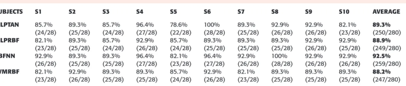
As for real-life applications, we individually test the accu-racy performance of each subject. Figure 5 plots the average accuracy of testing datasets from 10 subjects via different threshold score. Different color dotted lines mean the average accuracy of testing datasets using different training structures with thresholds from 0.1 to 0.9. Short vertical lines on each threshold point mean the standard deviation of average accu-racy from 10 subjects. According to the Figure 5 results, we have two major findings. One is that the classification accura-cy of four different models are increasing while the threshold is also increasing from 0.1 to 0.6 and then decreasing. Conse-quently, RBFNN model performs the best testing accuracy (92.5%) under threshold 0.6 and the local optimum threshold values 0.6 and 0.7 will lead to the better classification perfor-mance. Moreover, we collect the classification accuracy of each subject under threshold 0.6 in Table 2. The numerator value in brackets means the number of correct classified components and the denominator value means the totally 28 extracted components. The other finding is that SVMRBF
TABLE 1 Ten-fold cross validation accuracy of training datasets.
SUPERVISED METHODS ACCURACY RATE 6 STANDARD DEVIATION
MLPTAN 83.5% 6 0.0082 MLPRBF 83.8% 6 0.0133 RBFNN 90.6% 6 0.0085 SVMRBF 92.6% 6 0.0037 C1 C2 C3 C4 C5 C6 C7 C8 C9 C10 Weight Vectors (Ten Subjects) Testing Dataset Ten Classifiers Results via Thresholds Summation of Ten Classifier Results Desired Data Labels
FIGURE 4 Testing algorithm through ten-fold cross validation training classifiers.
1 0.95 0.9 0.85 0.8 0.75 0.7 0.65 0.6 0.55 0.5 0.45 0.4 0.1 0.2 0.3 0.4 0.5 0.6 0.7 0.8 0.9 Threshold MLPTAN MLPRBF RBFNN SVMRBF Accur acy
FIGURE 5 Average accuracy of testing datasets from 10 subjects via
(the black line) performs the more stable classi-fication performance. All classiclassi-fication accura-cies of 10 different thresholds are over 85%. Therefore, if we can not find the global opti-mum value of the threshold, we can use SVMRBF to be a general model of useful com-ponents selection. It can guarantee the
classifi-cation performance is 85% at least. In other words, 85% accuracy means that there are four misclassified components in 28 components.
In summary of training and testing results, we suggest that RBFNN model will be the better model for the automatic scheme of useful component selection. It can also perform the better predictive performance for real-life application. Regard-ing the optimal threshold of RBFNN model, we suggest set-ting value at 0.6 is enough to have better performance. Since the number of good components is much smaller than the bad components, the training process may give more importance to the noise components. We plan to explore the utility of data replication as well as generation of additional data through rotation or negation in the future investigation. In addition, we had applied the automatic classification system to the below case studies of driving cognition to automatically select the useful brain sources/independent components.
4. Case Studies: Driver’s Drowsiness Estimation in Long-term Driving
It has been widely accepted that the variation of human alertness, revealed on the changes of behavioral performance, was involved in alterations of the oscillatory brain activities in some specific brain regions (e.g. central, parietal and occipital areas etc.) and such fatigue related changes on brain rhythms can be assessed in terms of the electroencephalogram with Fourier methods and time-frequency analysis. Though abundant results in the litera-tures have shown that EEG traces could reflect changes of the alertness, EEG correlates of fluctuations in alertness from differ-ent experimdiffer-ents are still quite diverse. Specifically, the intensity of the alpha [39–40] or theta [41–43] band power was found respectively increased with the degradation of behavioral perfor-mance in different experiments. However, some studies reported that both theta and alpha band power were increased with the deleterious of the subjects’ performance [44–46]. Our previous studies also observed that the EEG frequency components forming the highest correlations with the long-term driving
per-formance were subject-dependent [19–21]. These discrepancies may due to the observed subjects’ drowsiness levels were not identical. For example, in a series of study investigating the corre-lations of human performance and alertness, subjects with increased theta activities performed longer response time [42–43] than the periods with augmented alpha activities [39]. Therefore, the aim of this study was to continuously assess the changes of the EEG rhythms from alertness to drowsiness for elucidating the exactly nature of the fatigue related EEG dynamics.
4.1 Subjects Performing in the Lane Keeping Driving Task Ten right-handed healthy (nine males, 18–28 years old) vol-unteers with normal or corrected to normal vision were paid to participate the lane keeping experiment. All subjects were free from neurological or psychological diseases and without drug or alcohol abuse. No subjects reported with sleep depri-vation at one day before the experiment. Subjects were required to have lunch at one hour before the experiment since it has been know that the drowsiness easily occurred during early morning, mid-afternoon, late nights and especial-ly after meal times [47]. Furthermore, it is also reported that the alertness is easily diminished within one-hour monoto-nous working during the above periods [48–49]. An informed consent was obtained from every subject before the experi-ment and the experiexperi-ment protocol was approved by the Insti-tutional Review Broad of Taipei Veterans General Hospital.
Each subject performed the experiment in the simulated realistic-driving environment. The four-lanes road of the VR scene were separated by a median strip and the distance between the left and right sides of the road was equally divided into 250 points (digitized into values 0–250), where the width of each lane and the car was 60 and 32 units, respectively. The refresh rate of highway scene was set at 60 Hz which can prop-erly emulate a car driving at a fixed speed of 100 km/hr on the highway. All scenes were updated according to the displacement of the car and the subject’s wheel handling. The car was randomly drifted away from the center of the cruising lane,
TABLE 2 Testing classification accuracy of each subject under threshold 0.6.
SUBJECTS S1 S2 S3 S4 S5 S6 S7 S8 S9 S10 AVERAGE MLPTAN 85.7% (24/28) 89.3% (25/28) 85.7% (24/28) 96.4% (27/28) 78.6% (22/28) 100% (28/28) 89.3% (25/28) 92.9% (26/28) 92.9% (26/28) 82.1% (23/28) 89.3%(250/280) MLPRBF 82.1% (23/28) 89.3% (25/28) 85.7% (24/28) 92.9% (26/28) 85.7% (24/28) 89.3% (25/28) 89.3% (25/28) 89.3% (25/28) 92.9% (26/28) 92.9% (25/28) 88.9%(249/280) RBFNN 92.9% (26/28) 89.3% (25/28) 89.3% (25/28) 96.4% (27/28) 82.1% (23/28) 96.4% (27/28) 92.9% (26/28) 100% (28/28) 92.9% (26/28) 92.9% (26/28) 92.5% (259/280) SVMRBF 82.1% (23/28) 92.9% (26/28) 89.3% (25/28) 89.3% (25/28) 85.7% (24/28) 92.9% (26/28) 82.1% (23/28) 89.3% (25/28) 89.3% (25/28) 89.3% (25/28) 88.2% (247/280)
RBFNN performs the best accuracy for the automatic
scheme of useful component selection. SVM with
RBF kernel can be as a general model due to its
stable accuracy.
which was controlled and triggered from the WTK program, to mimic the consequences of a non-ideal road surface. The inter-deviation intervals were varied from 5 to 10 sec and the car was deviated to either left or right side with the equal chance. This task required subjects to compensate the drifting by manipulat-ing the steermanipulat-ing to keep the car on the center of third cruismanipulat-ing lane (counted from left to right).
4.2 Brain Dynamics Changes from Alertness to Drowsiness
All subjects showed several periods of the fluctuated driving performances from small to large local driving errors (LDE), sometime even abandoning control of the steering during the 100-min driving task. Figure 6(A) showed that several fluctua-tions occurred in the typical LDE trajectory during the single session of subject 10. The sorted LDE curve of the single sub-ject (Fig. 6(B)) showed that LDE values were distributed from
0 to 70 and the majority of the LDE values were ranged between 0 and 30. Since only limited trails were with LDE values over 30 across 10 subjects, therefore, only trials with LDE values below 30 were selected for further analyzing. The responses to the drifting event were ranged from 500 to 6000 ms, which corresponded to the values of the LDE between 0 and 30. Thus, the LDE values lower than 3 indirectly indicated the subject was alert.
Ten subject’s cumulative percentage plots of the LDE with values from 0 to 30 showed in Fig. 6(C). Though the percent-age of the different drowsiness levels were varied across sub-jects, all subjects exhibited cognitive status from alertness to drowsiness. Figure 7 shows the grand means of the LDE sort-ed power spectra and the detail changes at the alpha- and the-ta-band spectra at the occipital (Fig. 7(A)), parietal (Fig. 7(B)) and frontal (Fig. 7(C)) IC clusters. In the occipital IC cluster, the dominant frequency band is shifted from alpha to theta band along with increases of the LDE indexes. For characteriz-ing the temporal changes of the LDE-related power spectra at the alpha- and theta-band in details, the temporal profile of the power changes at alpha- and theta-band are plotted against the LDE indexes shown at Fig. 7(D), 7(G). The changes of the alpha-band power show a non-monotonic profile along with the decreases of the alertness. Spe-cifically, the alpha-band power is linearly increased for the LDE index lower than 20 and then the power is slightly decreased for the LDE indexes between 20 and 30. The theta-band power shows a linearly increased from low LDEs to high LDEs. Similar changes on the LDE-sorted spectra are also observer at the parietal IC cluster but the variations of the EEG activities is weaker than that observed at the occipital IC cluster (as shown in Fig. 7(B)).
The peak intensities of the alpha- and theta-band power were significantly 1P , 0.052 lower than those observed at the occipital IC cluster (alpha: 1.2 vs 2.1; theta: 0.8 vs 1.5). Additionally, the rate of the spectral power increases at the alpha- and theta- band power are lower than those at the occipital cluster (alpha: 8 vs 5; theta: 13 vs 10). As for the frontal clus-ter, a significant power increase is showed around the 5 Hz at higher LDE values in the LDE-related spectra. Similar to the occipital and parietal clusters, the theta-band power is linearly increased with the increases of the LDEs. The alpha-band power is only increasing slightly along with the decreases of alertness at the frontal cluster. According to these results, 80 40 0 Local Dr iving Error 80 40 0 0 0 2,000 4,000 6,000 0 0 1,000 2,000 3,000 0 0 10 20 30 Local Dr iving Error 100 0 Time (s) Data Points
Local Driving Error (a) (b) (c) % T o tal Data P o ints (%)
FIGURE 6 (a) The time course of the local driving error during a sample one-hour session (S10). (b) Sorted local driving error values. (c) The cumulative percentage plots of LDE from 10 subjects showing all subjects exhibited different performance periods from alertness to drowsi-ness. Each color trace represented the cumulative percentage plot from a single subject.
Adaptive feature selection mechanism (AFSM) can
automatically select effective EEG features and
ICAFNN can accurately estimate driver’s individual
alertness level.
we used the alpha- and theta-band power as the EEG features from the occipital and parietal components and then applied to an adaptive feature selec-tion and ICA-Mixture-Model-based Fuzzy Neural Networks (ICAFNN) [50] to estimate the driver’s drowsiness level. 4.3 EEG-Based ICAFNN for Driver’s Drowsiness Estimation
In order to automatically select the drowsiness related features, an adaptive feature selection mechanism based on the correlation coefficients between log bandpower of the drowsiness related components and subject’s alertness level index (SALI) was proposed in this study. We use the cor relation spectra to illustrate the proposed adaptive feature selection mechanism (AFSM) [21]. After feature selection process, ICAFNN which was performed as the alertness level estimator in the study is a novel fuzzy neural network (FNN) and it can construct itself with an economic net-work size, and the learning speed as well as the modeling ability [50].
Experiment results shown in Table 3 are the selected features from 5 different subjects. The features selected by the method in [19] are also included in Table 3 for comparison. As can be seen, two methods might select different components. In general, the drowsiness-related regions are mainly in the parietal and occipital lobes. Optimal frequency bands were selected according to the
Occipital P o w er (dB) P o w er (dB) Parietal Frontal 4 0 4 0 4 5 –1 0 15 10 5
Frequency (Hz)0 Frequency (Hz)15 10 5 Frequency (Hz)15 10 5
30 0 LDE 30 0 30 5 0 10 20 30 –1 5 0 10 20 30 –1 5 0 10 20 30 –1 5 0 10 20 30 –1 5 0 10 20 30 –1 5 0 10 20 30 –1
Local Driving Error Alpha Theta P o w er (dB)
Significant Mean + SD Mean
15 10 0 3 15 10 5 0 3 15 10 0 LDE 3 3 3 3 3 3 (a) (d) (e) (f) (g) (h) (i) (b) (c)
FIGURE 7 The grand mean of the local driving error sorted EEG spectra of the occipital IC (a),
(d), and (g); parietal IC (b), (e), and (h); and frontal IC (c), (f), and (i). Upper: the grand mean of the error sorted power spectra normalized by subtracting the mean spectrum of the alert zero-error performance in each subject. Middle: The grand of the error sorted alpha-band power spectra of the three ICs across 10 subjects. The top insets showed the average scalp maps of the three ICs. Lower: The grand of the error sorted alpha-band power spectra of the three ICs across 10 subjects. Solid lines: The grand mean of the sorted alpha and theta-band power spectra. Dash lines: The grand mean plus the standard error of the sorted alpha and theta-band power spectra. Black horizontal thick line segments: alpha- and theta bands exhibit-ed significant ( p , 0.01) drowsy spectral power increases. Numbers indicated the correspond-ed local driving error values, which were the onsets of the drowsy spectral power significantly increased at the alpha and theta bands for the three ICs.
TABLE 3 Compared features with the method in [19] and the AFSM corresponding to different subjects.
SUBJECT1 SUBJECT2 SUBJECT3 SUBJECT4 SUBJECT5
SC ALP P LO T OF IC A C OM. B Y R EF [1 9 ] FREQ. BANDS 5 , 9 HZ 8 , 12 HZ 10 , 14 HZ 4 , 8 HZ 8 , 12 HZ SC ALP P LO T OF IC A C OM. B Y AF SM FREQ. BANDS 4 , 8 HZ 5 , 9 HZ 9 , 13 HZ 7 , 11 HZ 10 , 14 HZ
correlation coefficients between ICA power spectra and drowsiness index and iteratively testing by the linear regres-sion model (LRM) [19].
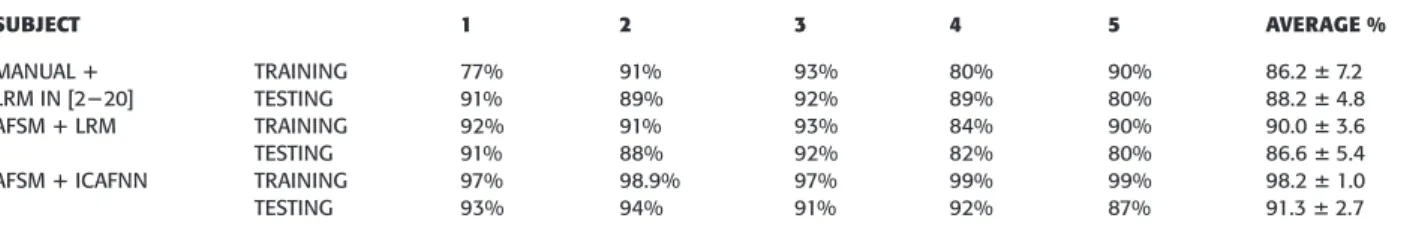
In order to compare the performance of these two feature selection methods, the features are used as inputs of the linear regression models for driver’s alertness level estimation, as shown in Table 4. The mean correlation between actual alert-ness level time series and within-session estimation by using the features selected by AFSM is 90%, whereas the mean corre-lation coefficient between actual alertness level and cross- session estimation is 86.6%. The average performance of the AFSM is closed to the performance using the optimal features. It can also be found that some testing results are better than the performance of the training sessions due to the repeatedly test-ing procedure. In addition, we fed the features selected by AFSM into the ICAFNN for subject’s alertness level estima-tion. The ICA weight matrices obtained from the training ses-sions were used to spatially filter the features in the testing sessions so that training/testing data were processed in the same way before feeding to the estimation models for the same sub-ject. Table 4 (bottom row) summarizes the performance of alertness level estimation obtained by the ICAFNN model across ten sessions of five subjects. The mean correlation between actual and estimated alertness level time series is 98.26 1.0%, whereas the mean correlation coefficient in cross-session testing is 91.36 2.7%.
5. Case Studies: Driver’s Distraction Effect Extraction in Dual-task Driving
Distraction and inattention of drivers have been identified as the main leading causes of car accidents and often affects driver’s attention ability. The U.S. National Highway Traffic Safety Administration has identified driver distraction as a high priority area about 20–30% [51]. Distraction during driving by whatever cause was a significant contributor to road traffic accidents [52–53]. Driving is a complex task in which several skills and abilities are involved simultaneously.
Reasons of distractions found during driv-ing were quite widespread, includdriv-ing eat-ing, drinkeat-ing, talking with passengers, using cell phones, reading, feeling fatigue, prob-lem-solving, and using in-car equipment. Recently, commercial vehicle operators with complex in-car technologies are also at increased risk since drivers may become increasingly dis-tracted in the years to come [54]. Some literatures studied the behavioral effect of driver’s distraction in car. It was shown by [55] based on measurement of the static completion time of an in-vehicle task. Similarly, the distraction effects caused by cellular phones during driving have been a focal point of recent in-car applications [56–57]. Experimental studies have been conducted to assess the impact of specific types of driver distraction on driving performance. Though these studies generally reported significant driving impairment [58], but simulator studies cannot provide information about the impact of these decrements of crashes resulting in hospital attendance of drivers. Therefore, in order to provide informa-tion before the occurrence of crashes, the drivers’ physiologi-cal responses were investigated. But to monitor drivers’ attention-related brain resources is still a challenge for researchers and practitioners in the field of cognitive brain research and human–machine interaction.
The main goal of this section was to investigate the brain dynamics related to distraction by using EEG and VR-based realistic driving environment. Unlike the previous studies, the designed experiment has three main characteristics. First, the SOA experimental design with the different appearance time of dual tasks (mathematical questions and unexpected car deviation) has the benefits to investigate the driver’s behavioral and physiological response under multiple condi-tions and multiple distracted levels. Second, the ICA-based advanced analysis methods were used to extract the artifact-free brain responses and related cortical location related to the single/dual task. Third, compared with single task, the interaction and effects of dual-task-related brain activities were also investigated.
5.1 Subjects Performing in the Dual-Task Driving Task Fifteen healthy participants (15 males), between 20 and 28 years of age, were recruited from the university population. They had normal or corrected-to-normal vision, were right
TABLE 4 Comparisons of different alertness level estimation approaches including linear regression models (LRM) using the features
selected by the method in [19], by AFSM, and the ICAFNN model using the features selected by AFSM for five different subjects.
SUBJECT 1 2 3 4 5 AVERAGE % MANUAL 1 LRM IN [2220] TRAINING 77% 91% 93% 80% 90% 86.2 6 7.2 TESTING 91% 89% 92% 89% 80% 88.2 6 4.8 AFSM 1 LRM TRAINING 92% 91% 93% 84% 90% 90.0 6 3.6 TESTING 91% 88% 92% 82% 80% 86.6 6 5.4
AFSM 1 ICAFNN TRAINING 97% 98.9% 97% 99% 99% 98.2 6 1.0
TESTING 93% 94% 91% 92% 87% 91.3 6 2.7
Reasons of driver’s distraction during driving were quite
widespread, including eating, drinking, talking with
passengers, using cell phones, reading, feeling fatigue,
problem-solving, and using in-car equipment.
handed, with driver’s license, and reported being free of psychiatric or neurological disorders. Written informed consent was obtained prior to the study. Each subject participated in four simulated work ses-sions. In each session, the subject sat in
front of the monitor with their hands on the steering wheel to control the car to stay in the center of the third lane (from the most left lane).
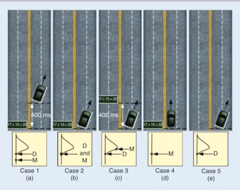
This section will investigate the distraction effects in dual-task conditions, two tasks including the unexpected car deviations and the mathematical questions were designed. In the driving task (car deviations), the car was constantly and randomly drifted from the center of the third lane. In this condition, the subjects needed to turn the steering wheel to let the car go back to the third land. It was for the sake of mimicking the consequences of driving on a non-ideal road surface. In the math task (mathematical questions), two-digit addition equations were presented in front of the subjects. The answers of the equations were designed to be either right or wrong. The subjects were asked to press the right or left button on the steering wheel when the equation was correct or wrong respectively. Moreover, the allotment ratios of correct or wrong equa-tions were both 50% and 50%. Especially, to investigate the effect of SOA between single- and dual- task conditions, the combinations of these two tasks were designed to pro-vide different distracting conditions to the subjects as shown in Fig. 8. Five cases were developed to
study the interaction of the two tasks. The bottom insets showed the onset sequences of two tasks.
5.2 Independent Component Clustering
EEG epochs were extracted from the recorded EEG signals. Then, the ICA was utilized to decompose the indepen-dent brain sources from EEG signals. Based on distraction effects, plenty of brain sources were involved in this experiment. For example, the motor component would be active when the subjects were trying to control the car with the steering wheel. In the mean-while, activations in the frontal compo-nent would appear and be related to attention. Therefore, ICA components including frontal and motor were selected for IC clustering based on their EEG characteristics.
At the first, IC clustering grouped massive components from multiple ses-sions and subjects into several signifi-cant clusters. The cluster analysis,
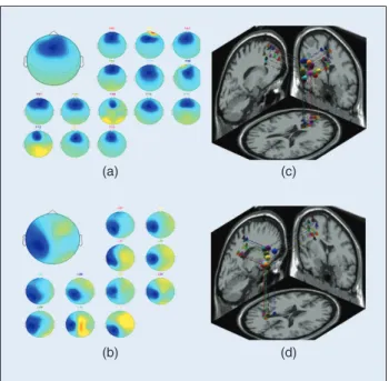
k-means, was applied to the normalized scalp topographies and power spectrum of all 450 (30 channels 3 15 subjects) components from the 15 subjects. Then, it identified at least 7 clusters of components having similar power spectrum and scalp projections. These 7 distinct component clusters accounted for frontal, central midline, parietal, left/right motor and left/right occipital, respectively. In this paper, frontal and left motor components were applied to analyze the distraction effects. Figure 9 showed the scalp maps and equivalent dipole source locations for two IC clusters, fontal and left motor. Based on this figures, the EEG sources of dif-ferent subjects in the same cluster were from the same physi-ological component.
5.3 Brain Dynamics Changes in Distraction Driving The cross-subject averaged ERSP in the frontal cluster corre-sponding to the five cases were shown in Fig. 10(a). Significant 1p , 0.012 power increases related to the math-task were observed in this figure. It demonstrated that the power increas-es in the frontal cluster were related to math task. The theta power increases in the three dual cases including case 1–3 were slightly different to each other. Comparing to single
400 ms 17 + 15 = 22 17 + 15 = 22 17 + 15 = 22 17 + 15 = 22 400 ms D D D Case 5 Case 4 Case 3 Case 2 Case 1 (e) (d) (c) (b) (a) D and M M M M
FIGURE 8 The illustration showed the relationship between the deviation onset and math occurred. D: deviation onset. M: math question onset. (a) Case 1: math was presented at 400 ms before the deviation onset. (b) Case 2: math and deviation occurred at the same time. (c) Case 3: math presented at 400 ms after the deviation onset. (d) Case 4: only math pre-sented. (e) Case 5: only deviation occurred. The bottom insets showed the onset sequences of two tasks.
For cross-subjects analysis, ICA component clustering
will be used to find the statistical and consistent
phenomena based on EEG characteristics.
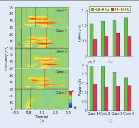
math task (case 4), the power in dual-task cases were stronger. Especially, the power increase in case1 was the strongest. In addition, the beta power increases which appeared only in the math-task and time-locked to mathematics onsets were induced by mathematical equations. The comparisons of the latency and total power in the four cases in Fig. 10(b) were given in Fig. 10(c). It demonstrated that the latency of power increases in both frequency bands were different with different time of SOA. The shortest latencies of power increases in both bands occurred in case 1. The longest latency of power increase in theta band occurred in case 4. It also demonstrated that the amount of power increases in theta band were differ-ent with differdiffer-ent time of SOA. The most significant power increase occurred in case 1.
6. Discussions
Noise removal in EEG signal is an essential and important step in any application of EEG. If independent component analysis is used for this purpose, then selection of useful independent components is the most crucial step. Typically this selection is done by human experts who decide looking at the scalp maps. This manual intervention not only makes it dependent on the availability and subjectivity of experts, but also it becomes a stumbling block in BCI and in any other real-time applications involving EEG. In this investiga-tion, we have demonstrated that machine learning approach-es can solve this problem to a great extent. In particular, we
have used four machine learning models to construct the automatic scheme for useful components selection. Al -though all of them are quite effective, RBFNN model will be the better model for the automatic scheme of useful component selection. It can also perform the better predic-tive performance for real-life application. Our investigation also indicates that the performance of a trained system on different subjects could be different, but this effect is not very severe and can be eliminated using fusion. Normally in a fusion scheme, decisions are made based on majority vot-ing. In our investigation, using a simple threshold score function we have found that higher vote does not necessari-ly mean better performance of a classifier system. Our inves-tigation indicates that it is possible to design a “universal system” for such job, given adequate training data. So far, there is no precise standard method to “automatically” select/reject the useful/artifact components and neuroscien-tists and psychologists always manually remove the noise components. When they are using EEGLAB open source toolbox, they are often confusing how to select the useful components and manually repeat the selection many times. Besides, EEGLAB has been “downloaded” at least 48,000 times and “applied” for many EEG-related studies. There-fore, such automatic selection system will be very useful for neuroscientists and psychologists to do the scientific research related to ICA application.
With the automatic brain sources classification system, we then investigated the neuro-physiological correlates of cogni-tive state changes using EEG and their relation to declining of performance during lane keeping driving task. In Fig. 7, the EEG a and u rhythm during periods of high error were significant stronger than during periods of low error. In detailed, the onset of the significant alpha-band power increases at three clusters was a little earlier than the theta-band power. These results would be suggested that previous controversial results may be partially caused by the different drowsiness levels between volunteers. Applying an adaptive EEG-based drowsiness estimation technology that combines the ICA, power spectrum analysis, adaptive feature selection mechanism (AFSM) and ICAFNN is also proposed to con-tinuously, indirectly estimate/predict fluctuations in human alertness level indexed by alertness level measurement, expressed as deviation between the center of the vehicle and the center of the cruising lane in a virtual-reality based driv-ing environment. The AFSM can automatically select effec-tive features based on the correlation analysis between the power spectra of drowsiness related components and the driving errors. The proposed ICAFNN can accurately esti-mate driver’s individual alertness level using ten sub-band power spectra of two ICA components selected by AFSM. The computational methods developed in this study can lead to on-line monitoring of human operators’ cognitive state in attention-critical settings.
Besides, we also investigated the effects of driver’s distraction in which different levels depends on the SOA experimental
(a) (c)
(b) (d)
FIGURE 9 The scalp maps and equivalent dipole source locations
after IC clustering for (a) the frontal components, (b) the left motor components, across 15 subjects. There were 14 subjects in the fron-tal cluster and 11 subjects in the left motor cluster. The bigger scalp map was the mean of the total component maps in the correspond-ing component cluster. The smaller maps were the individual scalp maps in the corresponding component cluster. The right panels (c) and (d) showed the 3-D dipole source locations (colored spheres) and their projections onto average brain images. The colored source locations were corresponding to its scalp map.
design. Cross-subject analysis was applied to prove that the appeared features were not restricted to specific subject or exper-iment. First, two main cortical areas including frontal area (which involved processing of mental tasks), somatosensory area (mu suppression phenomenon) were discussed. These cortical areas which had the difference between single- and dual-task cases would be selected to infer the relationship to the distraction effects. Then, the brain dynamic with behavior performance would be discussed to com-pare different distraction levels. The experimental results showed that behav-ioral and physiological (EEG) responses under multiple cases and multiple dis-tracted levels. The theta power increases in frontal area were higher in dual tasks than in single task. The phasic changes around the theta band for the case, which the math presented at 400 ms before the deviation onset, showed the strongest increase among all dual-task cases. This was because there was a first processing task in brain and subjects needed more brain source to manage the second task presented after the first task at 400 ms. Also, the latencies of the theta power increases were shifted along with the onset of math presented. The latency for the case, which the math presented at 400 ms before deviation, appeared was the shortest. In the beta band, the power increases were induced by the onsets of the math. In conclusion, the results also
suggested that the power increases of the frequency band, 4,7.8 Hz, in frontal area could be used as the index for early detecting driver’s distraction in the real driving.
7. Conclusion
This study had demonstrated that it is possible to develop-ing a “universal” machine for artifact removal in EEG sig-nals. Thus we applied such computational intelligence technology to investigate the brain computer interaction on driving cognition. Its implications for daily applications are also demonstrated through two common attention-re-lated driving studies: (1) cognitive-state monitoring of the driver performing the realistic long-term driving tasks; and (2) to extract the brain dynamic changes of driver’s distrac-tion effect during dual-task driving. The experimental results showed above of these studies will provide new insights into the understanding of complex brain functions of participants actively performing ordinary tasks in real-life applications, especially on driving cognition. They may
also be applied in future studies to elucidate the limitations of normal human performance in repetitive task environ-ments and may inspire more detailed study of changes in cognitive dynamics in brain-damaged, diseased or geneti-cally abnormal individuals. Furthermore, the applications on driving cognition would have many potential diverse research fields in the operational environment such as com-putational intelligence, cognitive neuroscience, human fac-tors and brain computer interfaces.
Acknowledgment
The authors would like to greatly thank our international collaborators, Doctors T. P. Jung, J. R. Duann, and R. S. Hunag in University of California, San Diego, for their sug-gestions and consultation, and also thank S. A. Chen, T. Y. Huang, J. L. Jeng, H. S. Huang, and T. T. Chiu for their devel-oping and operating the experiments. This work was in part supported by the Aiming for the Top University Plan of National Chiao Tung University, the Ministry of Education, 30 20 10 30 20 10 30 20 10 F requency (Hz) 30 20 10 30 20 10 0 –0.5 0.5 1.5 Time (s) (a) (b) ×103 (c) 2.5 3.5 Case 1 Case 2 Case 3 Case 4 Case 5 6 –6 1.5 1.0 0.5 0 2.5 2.0 1.5 1.0 P o w er (dB) Latency (s) 0.5 0
Case 1 Case 2 Case 3 Case 4 4.5–9 Hz 11–15 Hz
FIGURE 10 (a) The ERSP images of frontal cluster for five cases. The right column showed the onset sequences of two tasks. Color bars showed the magnitude of ERSPs. Red solid lines showed the onset of math. Red dashed lines showed the mean of response time to math. Blue solid lines showed the onset of deviation. Blue dashed lines showed the mean of response time to deviation. The red circle pointed by red arrow in case 2 means that the red solid line and blue solid line were on the same position. Latencies were calculated from cross-subject averaged ERSP images of the frontal component in (b). The opened bars represented the latencies which were counted from the math onset to the first time of power increase in theta (4.5,9 Hz) band. The gray bars represented these latencies in beta (11,15 Hz) band. The comparison of total power in cross-subject (14 subjects) averaged ERSP images in clus-tered frontal cluster between cases was shown in (c). The amount of total power was calculat-ed by adding all the power increases in the same period and frequency band. The opencalculat-ed bars represented the total power in the theta band. The gray bars represented the total power in the beta band.
Taiwan, under Contract 98W962 and in part supported by the National Science Council, Taiwan, under Contracts NSC 97-2627-E-009-001.
References
[1] A. Hyvarinen, J. Karhunen, and E. Oja, Independent Component Analysis. New York: Wiley, 2001.
[2] A. J. Bell and T. J. Sejnowski, “An information-maximization approach to blind sepa-ration and blind deconvolution,” Neural Comput., vol. 7, pp. 1129–1159, 1995. [3] T. W. Lee and T. J. Sejnowski, “Independent component analysis for sub-Gaussian and super-Gaussian mixtures,” in Proc. 4th Joint Symp. Neural Computation, vol. 7. La Jolla, CA: Univ. of California, San Diego, 1997, pp. 132–139.
[4] A. Delorme and S. Makeig, “EEGLAB: An open source toolbox for analysis of single-trial EEG dynamics including independent component analysis,” J. Neurosci. Methods, vol. 134, pp. 9–21, 2004.
[5] C. Jutten and J. Herault, “Blind separation of sources I. An adaptive algorithm based on neuromimetic architecture,” Signal Process., vol. 24, pp. 1–10, 1991.
[6] P. Comon, “Independent component analysis—A new concept?” Signal Process., vol. 36, pp. 287–314, 1994.
[7] M. Girolami, “An alternative perspective on adaptive independent component analy-sis,” Neural Comput., vol. 10, pp. 2103–2114, 1998.
[8] T. W. Lee, M. Girolami, and T. J. Sejnowski, “Independent component analysis us-ing an extended infomax algorithm for mixed sub- and super-Gaussian sources,” Neural Comput., vol. 11, pp. 606–633, 1999.
[9] T. P. Jung, C. Humphries, T. W. Lee, S. Makeig, M. J. McKeown, V. Iragui, and T. J. Sejnowski, “Extended ICA removes artifacts from electroencephalographic recordings,” Adv. Neural Inform. Process. Syst., vol. 10, pp. 894–900, 1998.
[10] T. P. Jung, S. Makeig, W. Westerfield, J. Townsend, E. Courchesne, and T. J. Se-jnowski, “Analysis and visualization of single-trial event-related potentials,” Hum. Brain Mapp., vol. 14, no. 3, pp. 166–185, 2001.
[11] M. Naganawa, Y. Kimura, K. Ishii, K. Oda, K. Ishiwata, and A. Matani, “Extraction of a plasma time-activity curve from dynamic brain pet images based on independent component analysis,” IEEE Trans. Biomed. Eng., vol. 52, pp. 201–210, Feb. 2005. [12] R. Liao, J. L. Krolik, and M. J. McKeown, “An information-theoretic criterion for intrasubject alignment of FMRI time series: Motion corrected independent component analysis,” IEEE Trans. Med. Imag., vol. 24, pp. 29–44, Jan. 2005.
[13] W. Wierville, J. G. Casali, and B. S. Repa, “Driver steering reaction time to abrupt-onset crosswind, as measured in a moving-base driving simulator,” Hum. Factors, vol. 25, no. 1, pp. 103–116, 1983.
[14] G. Reymond, A. Kemeny, J. Droulez, and A. Berthoz, “Role of lateral acceleration in curve driving: Driver model and experiments on a real vehicle and a driving simulator,” Hum. Factors, vol. 43, pp. 483–495, 2001.
[15] E. L. Groen, I. P. Howard, and B. S. Cheung, “Inf luence of body roll on visually induced sensation of self-tilt and rotation,” Perception, vol. 28, pp. 287–297, 1999. [16] C. T. Lin, I. F. Chung, L. W. Ko, Y. C. Chen, S. F. Liang, and J. R. Duann, “EEG-based assessment of driver cognitive responses in a dynamic virtual-reality driving envi-ronment,” IEEE Trans. Biomed. Eng., vol. 54, no. 7, pp. 1349–1352, 2007.
[17] C. T. Lin, L. W. Ko, J. C. Chiou, J. R. Duann, R. S. Huang, T. W. Chiu, S. F. Liang, and T. P. Jung, “Noninvasive neural prostheses using mobile and wireless EEG,” Proc. IEEE, vol. 96, no. 7, pp. 1167–1183, 2008.
[18] C. T. Lin, R. C. Wu, T. P. Jung, S. F. Liang, and T. Y. Huang, “Estimating alertness level based on EEG spectrum analysis,” EURASIP J. Appl. Signal Process., vol. 2005, no. 19, pp. 3165–3174, Mar. 2005.
[19] C. T. Lin, R. C. Wu, S. F. Liang, W. H. Chao, Y. J. Chen, and T. P. Jung, “EEG-based drowsiness estimation for safety driving using independent component analysis,” IEEE Trans. Circuits Syst. I: Reg. Pap., vol. 52, pp. 2726–2738, 2005.
[20] C. T. Lin, Y. J. Chen, R. C. Wu, S. F. Liang, and T. Y. Huang, “Assessment of driver’s driving performance and alertness using EEG-based fuzzy neural networks,” in Proc. IEEE Int. Symp. Circuits and Systems, 2005, pp. 152–155.
[21] C. T. Lin, L. W. Ko, I. F. Chung, T. Y. Huang, Y. C. Chen, T. P. Jung, and S. F. Liang, “Adaptive EEG-based alertness estimation system by using ICA-based fuzzy neural networks,” IEEE Trans. Circuits Syst. I: Reg. Pap., vol. 53, no. 11, pp. 2469–2476, 2006. [22] C. T. Lin, L. W. Ko, Y. H. Lin, T. P. Jung, S. F. Liang, and L. S. Hsiao, “EEG activi-ties of dynamic stimulation in VR driving motion simulator,” Lect. Notes Artif. Intell., vol. 4562, pp. 551–560, 2007.
[23] C. T. Lin, T. T. Chiu, T. Y. Huang, C. F. Chao, W. C. Liang, S. H. Hsu, and L. W. Ko, “Assessing effectiveness of various auditory warning signals in maintaining drivers’ attention in virtual reality-based driving environments,” Percept. Motor Skills, vol. 108, pp. 825–835, June 2009.
[24] S. Makeig, A. J. Bell, T. P. Jung, and T. J. Sejnowski, “Independent component analysis of electroencephalographic data,” Adv. Neural Inform. Process. Syst., pp. 145–151, 1996. [25] T. P. Jung, C. Humphries, T.-W. Lee, S. Makeig, M. J. McKeown, V. Iragui, and T. J. Sejnowski, “Extended ICA removes artifacts from electroencephalographic recordings,” Adv. Neural Inform. Process. Syst., pp. 894–900, 1998.
[26] P. LeVan, E. Urrestarazu, and J. Gotman, “A system for automatic artifact removal in ictal scalp EEG based on independent component analysis and Bayesian classification,” Clin. Neurophysiol., vol. 117, pp. 912–927, 2006.
[27] C. A. Joyce, I. F. Gorodnitsky, and M. Kutas, “Automatic removal of eye movement and blink artifacts from EEG data using blind component separation,” Psychophysiology, vol. 41, pp. 313–325, 2004.
[28] Y. Li, Z. Ma, W. Lu, and Y. Li, “Automatic removal of the eye blink artifact from EEG using an ICA-based template matching approach,” Physiol. Measure., vol. 27, pp. 425–436, 2006.
[29] R. Vigario, “Extraction of ocular artefacts from EEG using independent component analysis,” Electroencephalogr. Clin. Neurophysiol., vol. 103, pp. 395–404, 1997.
[30] A. Flexer, H. Bauer, J. Pripf l, and G. Dorffner, “Using ICA for removal of ocular artifacts in EEG recorded from blind subjects,” Neural Netw., vol. 18, pp. 998–1005, 2005.
[31] T. P. Jung, S. Makeig, C. Humphries, T. W. Lee, M. J. McKeown, V. Iragui, and T. J. Sejnowski, “Removing electroencephalographic artifacts by blind source separation,” Psychophysiology, vol. 37, pp. 163–178, 2000.
[32] D. Mantini, M. G. Perrucci, S. Cugini, A. Ferretti, G. L. Romani, and C. Del Gratta, “Complete artifact removal for EEG recorded during continuous fMRI using indepen-dent component analysis,” Neuroimage, vol. 34, pp. 598–607, 2007.
[33] P. J. Allen, O. Josephs, and R. Turner, “A method for removing imaging artifact from continuous EEG recorded during functional MRI,” Neuroimage, vol. 12, pp. 230–239, 2000.
[34] P. J. Allen, G. Polizzi, K. Krakow, D. R. Fish, and L. Lemieux, “Identification of EEG events in the MR scanner: The problem of pulse artifact and a method for its subtrac-tion,” Neuroimage, vol. 8, pp. 229–239, 1998.
[35] M. J. McKeown, S. Makeig, G. G. Brown, T. P. Jung, S. S. Kindermann, A. J. Bell, and T. J. Sejnowski, “Analysis of fMRI data by blind separation into independent spatial components,” Hum. Brain Mapp., vol. 6, no. 3, pp. 160–188, 1998.
[36] H. S. Huang, N. R. Pal, L. W. Ko, and C. T. Lin, “Automatic identification of useful independent components with a view to removing artifacts from EEG signal,” in Proc. Int. Joint Conf. Neural Networks (IJCNN’09), Atlanta, GA, June 14–19, 2009.
[37] H. S. Huang, N. R. Pal, L. W. Ko, and C. T. Lin, “An automatic scheme for useful independent components selection in EEG signals,” IEEE Trans. Inform. Technol. Biomed., submitted for publication.
[38] S. Haykin, Neural Networks: A Comprehensive Foundation. Englewood Cliffs, NJ: Prentice-Hall, 1999.
[39] R. S. Huang, T. P. Jung, A. Delorme, and S. Makeig, “Tonic and phasic electroen-cephalographic dynamics during continuous compensatory tracking,” NeuroImage, vol. 39, pp. 1896–1909, 2008.
[40] J. Santamaria and K. H. Chiappa, “The EEG of drowsiness in normal adults,” J. Clin. Neurophysiol., vol. 4, no. 4, pp. 327–382, 1987.
[41] J. Beatty, A. Greenberg, W. P. Deibler, and J. O’Hanlon, “Operant control of oc-cipital theta rhythm affects performance, in a radar monitoring task,” Science, vol. 183, pp. 871–873, 1974.
[42] S. Makeig and T. P. Jung, “Tonic, phasic, and transient EEG correlates of auditory awareness in drowsiness,” Cogn. Brain Res., vol. 4, no. 1, pp. 15–25, July 1996. [43] T. P. Jung, S. Makeig, M. Stensmo, and T. J. Sejnowski, “Estimating alertness from the EEG power spectrum,” IEEE Trans. Biomed. Eng., vol. 44, pp. 60–69, 1997. [44] A. Campagne, T. Pebayle, and A. Muzet, “Correlation between driving errors and vigilance level: inf luence of the driver’s age,” Physiol. Behav., vol. 80, no. 4, pp. 515–524, 2004.
[45] G. Kecklund and T. Akerstedt, “Sleepiness in long distance truck driving: an ambula-tory EEG study of night driving,” Ergonomics, vol. 36, no. 9, pp. 1007–1017, 1993. [46] L. Torsvall and T. Akerstedt, “Sleepiness on the job: Continuously measured EEG changes in train drivers,” Electroencephalogr. Clin. Neurophysiol., vol. 66, no. 6, pp. 502–511, 1987.
[47] D. Benton and P. Y. Parker, “Breakfast, blood glucose, and cognition,” Amer. J. Clin. Nutrition, vol. 67, pp. 772S–778S, 1998.
[48] J. Hendrix, “Fatal crash rates for tractor-trailers by time of day,” in Proc. Int. Truck and Bus Safety Research and Policy Symp., 2002, pp. 237–250.
[49] H. Ueno, M. Kaneda, and M. Tsukino, “Development of drowsiness detection system,” in Proc. Vehicle Navigation and Information Systems Conf., Sept. 1994, vol. 31, pp. 15–20. [50] C. T. Lin, W. C. Cheng, and S. F. Liang, “An on-line ICA-mixture-model-based self-constructing fuzzy neural network,” IEEE Trans. Circuits Syst. I, vol. 52, no. 1, pp. 207–221, Jan. 2005.
[51] A. R. Thomas, “Driver distraction: A review of the current state-of-knowledge,” Nat. Highway Traffic Saf. Admin. Veh. Res. Test Center, DOT F 1700.7, 2008, pp. 8–72.
[52] T. Horberry, J. Anderson, M. A. Regan, T. J. Triggs, and J. Brown, “Driver distrac-tion: The effects of concurrent in-vehicle tasks, road environment complexity and age on driving performance,” Accid. Anal. Prev., vol. 38, pp. 185–191, 2006.
[53] C. J. D. Patten, A. Kircher, J. stlund, and L. Nilsson, “Using mobile telephones: Cognitive workload and attention resource allocation,” Accid. Anal. Prev., vol. 36, pp. 341–350, 2004.
[54] T. Dukic, L. Hanson, and T. Falkmer, “Effect of drivers’ age and push button loca-tions on visual time off road, steering wheel deviation and safety perception,” Ergonomics, vol. 49, pp. 78–92, 2006.
[55] L. Tijerina, S. Johnston, E. Parmer, M. D. Winterbottom, and M. Goodman, “Driver distraction with route guidance systems,” Nat. Highway Traffic Saf. Admin., Tech. Rep. DOT HS 809-069, 2000.
[56] P. A. Hancock, M. Lesch, and L. Simmons, “The distraction effects of phone use dur-ing a crucial drivdur-ing maneuver,” Accid. Anal. Prev., vol. 35, pp. 501–541, 2003. [57] D. L. Strayer, F. A. Drews, and W. A. Johnston, “Cell phone-induced failures of visual attention during simulated driving,” J. Exp. Psychol., vol. 9, pp. 23–32, 2003. [58] D. Crundall, E. V. Loon, and G. Underwood, “Attraction and distraction of attention with roadside advertisements,” Accid. Anal. Prev., vol. 38, pp. 671–677, 2006.