區域經濟協定與雙邊貿易

全文

(1)國立高雄大學應用經濟學系碩士班碩士論文. 區域經濟協定與雙邊貿易 Regional Economic Agreements and Bilateral Trade Flows. 研究生：林鉦翰撰指導教授：鄭義暉博士. 中華民國一○○年一月. .

(2) 誌謝辭首先感謝全家人以及朋友給我的支持，尤其是老哥常來高雄支持跟鼓勵我，這些支持跟鼓勵讓我在歷經兩年多的時間讓碩士生涯總算告一段落。當然，在此最感謝的是我指導教授鄭義暉教授這兩年多的細心指導以及給予我更多課業外的知識使我研究生生涯充實許多，讓我不只在經濟學上獲取知識外，更能讓我了解如何使研究生的生活不只是做研究還有更多更重要的事是畢業前要去學會。另外要感謝這兩年常常陪我聊天談心的同學，這兩年常陪我吃飯還有互相鼓勵的同學明正以及總是會一起打氣的同學聖傑。還有也特別感謝珮華跟正宜學妹在論文之外總是可以給來很多歡樂以及陪我聊天，此外也感謝口試委員王俊傑老師跟佘志民老師對於本論文有多建議使論文能夠更為完備。最後要感謝家人，這一路上煎熬的碩士生活因為有你們的默默支持才能使我總算能順利畢業。林鉦翰謹誌 2011 年暖冬于高雄. 1 .

(3) 區域經濟協定與雙邊貿易 . 指導教授：鄭義暉博士國立高雄大學應用經濟學系. 學生：林鉦翰國立高雄大學應用經濟學系碩士班. 摘要近年來國際上各國透過簽訂自由貿易協定以進行區域經濟整合，在區域內消除部分貿易障礙及非貿易障礙，並冀藉以增進會員國間之貿易量或福利。本研究利用 1986-2008 年國際間雙邊貿易量來探討影響雙邊貿易之決定因素。針對區域經濟體的虛擬變數上，本研究選取北美自由貿易區、歐盟、東南亞自由貿易區及南方共同市場，使用的計量模型則採傳統的跨部門模型（PCS）、雙邊固定效果模型（FE2）、三邊固定效果模型（FE3）及一般化固定效果模型（FEG），實證結果顯示，若以 AIC 和 BIC 的判斷準則下，模型 FE2 最具有解釋力。此外，本研究更進一步討論不同計量模型 FE2 及 FE3 的截距項，針對不同估計法的特定效果的影響進行評估。. 關鍵字: 雙邊貿易流量、貿易引力模型、區域經濟整合. i .

(4) Regional Economic Agreements and Bilateral Trade Flows . Advisor：Dr. I-Hui Cheng Department of Applied Economics National University of Kaohsiung MA Student：Cheng-Han Lin Department of Applied Economics National University of Kaohsiung. Abstract The objective of this dissertation is to study the effects of regional economic agreements on bilateral trade flows. By using various specifications of gravity-type model, namely the pooled cross section (PCS), two-way fixed effects (FE2), three-way fixed effects (FE3) and generalized fixed effects (FEG) model, the study focuses on five major regional economic agreements, the EU, EURO, NAFTA, AFTA, and MERCOSUR. For the model selection, the study uses the AIC and BIC information criteria, and suggests that model FE2 is preferred. The study further investigates the difference of intercepts estimated from models FE2 and FE3. Keywords：Bilateral trade, Gravity model, Regional economic integration. ii .

(5) Table of Contents. i. 中文摘要. ii. Abstract. iii. Table of Contents. iv. List of Tables. I.. Introduction. 1. II.. The Literature. 3. III.. Contemporary World Trade. 8. IV.. The Empirical Models and Estimation Results. 11. 4.1 The Empirical Models. 11. 4.2 The Data. 14. 4.3 Main Estimation Results. 16. 4.4 The Results of a Further Study on Country-specific Effects. 19. The Conclusions. 21. V.. References. 23. Data Appendix. 47. iii . .

(6) List of Tables Table 1. The total value of exports in different geographical regions. 27. Table 2. The total value of imports in different geographical regions. 28. Table 3. Leading exporters and importers in world merchandise trade, 2008. 29. Table 4. Merchandise trade of the United States by origin and destination, 2008. 30. Table 5. Merchandise trade of the European Union (27) by origin and destination, 2008. 31. Table 6 . Merchandise trade of Japan by origin and destination, 2008. 32. Table 7 . Exports of trade groups. 33. Table 8 . Imports of trade groups. 34. Table 9 . Variables and data sources. 35. Table 10 List of 41 exporting and 57 importing countries. 36. Table 11 Trade blocs and selected member countries. 37. Table 12 List of developed and developing countries and country dummies. 38. Table 13 Main regression results for various models. 40. Table 14 Estimated exporter and importer dummies and country-pair dummies 41. iv . .

(7) I. Introduction In an open economy, volumes of trade play an important role in determining the aggregate welfare, which is counted by the summation of total consumption, investment, government expenditure and net foreign trade. This dissertation uses the gravity model of trade which is the most popular approach in recent decades to study the effects of bilateral trade volume. Regional trading agreements (RTAs) have been one of the most important factors determining trade volumes. In order to eliminate the trade barrier, more and more countries intend to sign preferential trading agreements (PTAs). According to the degree of economic integration among members, trading agreements are classified into four categories, including free trade areas (FTA), customs union (CU), common market and monetary union. For example, in America, the main RTAs include the Common Markets of the South (MERCOSUR), the North American Free Trade Agreement (NAFTA), the Central American Common Market (CACM) and Latin America Free Trade Association (LAFTA). In Africa, the Common Market of Eastern and Southern Africa (COMESA) are acting. In Asia, the Association of Southeast Nations (ASEAN) and then the ASEAN Free Trade Area (AFTA) already enter into force. The main purpose of this study is to discuss how economics of trading blocs and economic similarity affect trade volumes. It focuses on the following issues: (a) to use traditional and modified models of gravity type to estimate bilateral trade, (b) to consider whether the bilateral trade flows are affected by different trading agreements, (c) to study further how different levels of economic development affects bilateral trade flows, (d) to consider if different level of trade similarity has impact on bilateral. 1 . .

(8) trade, and (e) to discuss the estimation results between different models. This dissertation is organized as follows. Section Two section presents the literature reviews. Section Three describes the current world trade. Section Four introduces the estimation data and models, and then discusses the empirical analysis. Finally, the conclusions and suggestions for further study are made in Section Five.. 2 . .

(9) II.. The Literature. In early 1960s, Tinbergen (1962) and Pöyhönen (1963) introduced the gravity model of international trade to study bilateral trade flows of two countries. The gravity model of international trade explains that trade flows between countries increase in the size of two trading partner countries, and decrease in the cost of transportation between them (as measured by the distance between their economic centers). Linnemann (1966) then modified the standard gravity model and added population as an additional measure of country size, i.e. the population size has a significant and negative impact on trade flows.1 It is also common to specify a gravity model including per capita income, which captures the similar effect of purchasing power on trade flows. Brada and Mendez (1983) adopted per capita national incomes as exogenous variables to study the effects on trade flows. By using the specification of the gravity model in which consist of either population or per capita income, the objective is to allow for non-homothetic preferences in the importing country, and to replace for the capital/labor ratio in the exporting country (Bergstrand, 1989). In general, the gravity model is commonly extended to include other explanatory variables to capture the effects of regional trading groups, political blocs, and various trade distortions. The events and policies modeled as deviations from the value of trade predicted by the baseline gravity model are captured by dummy variables.2 Anderson (1979) considered the properties of the expenditure system to analyze the gravity model. Two cases of product differentiation are discussed in his study: the Cobb-Douglas (C-D) and the constant-elasticity-of-substitution (CES) preferences. Bergstrand (1985) firstly included the variables of prices, and uses CES preferences to derive the gravity equation.                                                              1 2. For the survey, see Oguledo and MacPhee (1994). It should be noted in Eichengreen and Irwin (1998), the gravity model is acting as “workhorse of empirical studies of (regional integration) to the virtual exclusion of other approaches.” 3 . .

(10) Moreover, Bergstrand (1989) used the CES preferences, i.e. products are differentiated among firms rather than countries, to consider the role of monopolistic competition in international trade. Baier and Bergstrand (2001), Eaton and Kortum (2002), and Anderson and van Wincoop (2003) consider that prices always adjust to equate supply and demand. Deardorff (1998) considered two cases of the gravity model, a frictionless trade and impeded trade cases, and derived bilateral trade relationship with the Heckscher-Ohlin theory. In his paper, he showed that in the presence of transportation costs and tariffs, the pattern of trade flows on a C.I.F. basis is the same form with the frictionless trade case. With C-D preferences, trade flows on an F.O.B. basis of the gravity equation are represented, weighed with the iceberg-form transportation costs. With the CES preferences, the measurement of the value of trade flows on an F.O.B. basis is more complicated. Trade flows are derived as the function of the incomes of importing and exporting countries, exporter’s share of world income, the relative and average distances from suppliers. By the assumption of the identical and homothetic preferences without transportation costs and tariffs, both Anderson (1979) and Deardorff (1998) showed that the gravity model is the product of the two countries’ incomes divided by the sum of world income. Bergstrand (1985) further provided an additional assumption of perfect substitutability of goods internationally in production and consumption, showing that the value of a trade flow is simple one half of the square root of the product of the two countries’ incomes. The reason why we study the impact of regional economic integration on trade flows is that trade flow effects play an important role to determine the aggregate welfare change for members of a regional integration agreement. Viner (1950) introduced the concepts of trade creation and trade diversion effects to identify situations under which. 4 .

(11) a customs union (CU) is welfare-increasing or welfare-reducing.3 He considered that the tariff decreases or elimination between members as part of a free trade agreement while maintaining its tariffs against other countries. The issue of testing the effects of regional integration agreement on trade is of great concern due to the increasing tendency of countries to form preferential trading agreements (PTA) in recent decades. The most popular method in recent empirical literature is to estimate trade flows by the use of a dummy variable to identify regional economic integration (REI) partners with simple gravity models, i.e., a dummy variable takes the value of one if both trading partners interact in the same trading bloc and zero otherwise.4 Aitken (1973) firstly included one dummy variable to the gravity model to evaluate the intra-bloc effect of a REI, showing that the European Community (EC) has statistically significant impact on trade flow between members.5 Brada and Mendez (1983) used a gravity model to examine the REI effect, showing that economic integration tends to increase trade between member countries, and their per capita incomes and decreases with the distance between them. Frankel (1995) further included additional dummy variables for country pair sharing a common land border and common language, and trade bloc dummy variables to evaluate the effect of free trade agreements. Bayoumi and Eichengreen (1997) adopted two dummy variables for each REI to evaluate the separate effects on intra-bloc and extra-bloc trade. One of the two dummy variables is set to be one if the two countries join the same trade blocs. Another dummy variable is set to be one if either country is in the blocs. Thus, the coefficients can be                                                              3. 4 5. For a country, trade creation means that joining a customs union would have advantages if joining results in the replacement of high-cost domestic production by imports from a lower-cost country within the union. By contrast, trade diversion means that joining leads to a shift in domestic consumption from a low-cost country outside the customs union to a higher-cost country inside the union, the home country may suffer. See Aitken (1973), Winters (1992), Bayoumi and Eichengreen (1997) and Sapir (1997) for the analysis of integration schemes in Western Europe. Also see Abrams (1980) and Brada and Mendez (1985). 5 . .

(12) used to evaluate the trade creation and trade diversion. The basic gravity model can also be extended to include three sets of dummy variables for each trade bloc: one captures intra-bloc trade, the second captures imports by members from all countries (include members and non-members), and the third captures exports by bloc members to all countries (see Cheng and Tsai, 2008). Hummels and Levinsohn (1995) considered if the underlying theoretical model is correct, i.e. they considered that the model might not fit the data in every year for every country-pair. In addition, Mátyás (1997) used a triple-indexed specification of the gravity model, including the year dummy and two sets of country-specific effects entailing fixed effects for both the exporting country. Egger (2000) focused on the random effects gravity approaches, and considered the fixed effects model given both along intuitive and econometric lines with Hausman test. Egger and Pfaffermayr (2003) reconsidered that specification of a panel gravity model. According to their suggestion, a generalized gravity model should consist of main effects (exporter, importer and time) as well as time invariant exporter-by-importer (bilateral) interaction effect. Baltagi et al. (2003) further considered full interaction effects into the model of the bilateral trade flows. By doing so, they found empirical support for the New Trade Theory and Linder’s hypothesis. Baltagi et al. (2003) also considered a pretest estimator based on two Hausman tests as an alternative to choose the fixed effects or random effects estimators for panel data model. Subramanian and Wei (2007) suggested that WTO does promote trade. According to their study, industrial countries participate more actively than developing countries in trade negotiation. And bilateral trade is greater if two both countries undertake liberalization than when only one does. Magee (2008) adopted the effects of regional agreements on trade flows, controlling for country pair, importer-year, and exporter-year fixed effects. He argued that controlling for the fixed effects reduces the estimated trade 6 .

(13) impacts of regional agreements. Baier and Bergstrand (2007) considered that trade policy is not an exogenous variable, i.e. it can be a econometrically the endogenous variable of FTAs. They found that the endogenous variable of FTAs has significant effects. Egger et al. (2008) also found a particularly strong effect of endogenous regional trading agreements (RTAs) on intra-industry trade in a difference-in-difference analysis, indicating that RTA membership might reduce inter-industry trade. Egger and Larch (2008) examined a pair of countries on bilateral trade, showing that pre-existing PTAs increase the probability of a country-pair entering a bilateral PTA. Baier and Bergstrand (2009) used the cross-section estimates of long-run treatment effects and matching econometrics to study the effects of free trade agreements on members’ bilateral trade flows.. 7 .

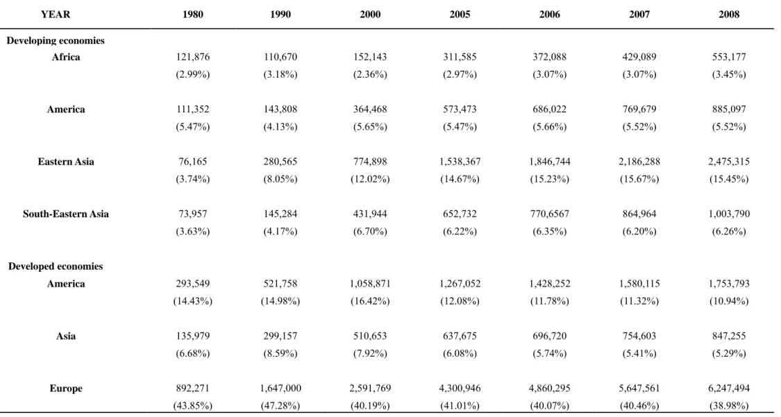
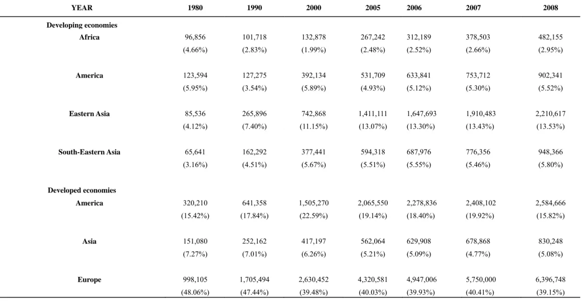
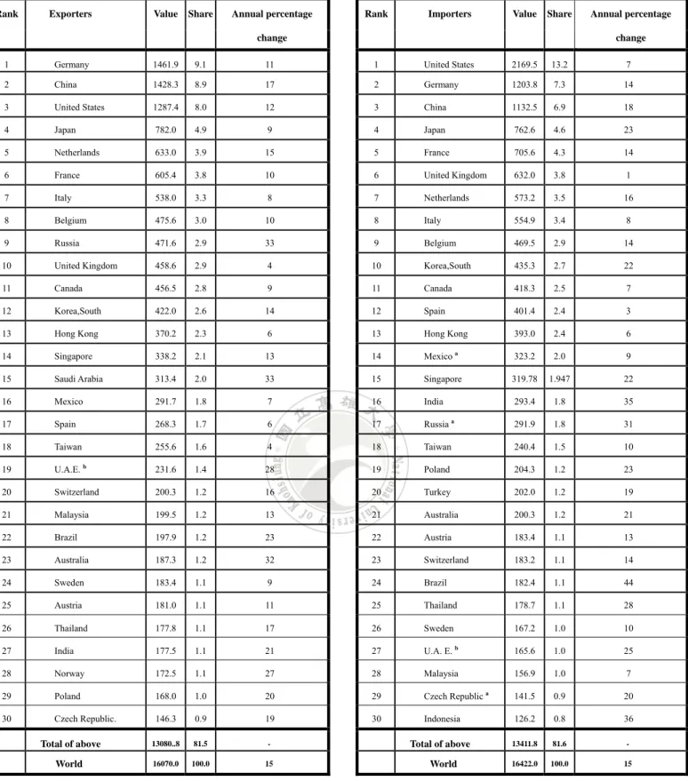
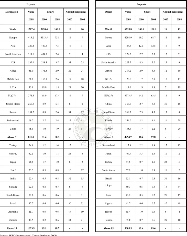
(14) III. Contemporary World Trade During the period between year 1980 and 2008, all the values of exports and imports in different geographical regions have grown significantly (Tables 1 and 2). Since 1980, the shares of exports and imports of Eastern Asia relative to world trade are increasingly stable. As shown in Table 1, the share of the Eastern Asia’s exports relative to world trade is nearly 15.45 percent in year 2008. During the same period, the export share of South-eastern Asia has risen approximately two times, from 3.63 percent in year 1980 to 6.26 percent in year 2008, increasing fast up to 1,003,790 millions of dollars from 73,957 millions of dollars during year 1980 to year 2008. In contrast, the shares of exports in developed Asian and developed American countries have decreased during this period. As illustrated in Table 2, since year 1980 the shares of imports in different geographical regions also have shown similar trend as exports except America. The share of the developed Europe’s imports relative to world trade is nearly 39.15 per cent in year 2008. It still ranks the first in the world trade but is 8 per cent lower than that in year 1980, increasing to 6,396,748 millions of dollars from 998,105 millions of dollars during the same period. The share of the developed America’s imports relative to world trade has decreased during year 2000 to year 2008. The import share of developing Eastern Asia has risen almost four times, from 4.12 percent in year 1980 to 13.53 percent in year 2008, increasing to 2,210,617 millions of dollars from 85,536 millions of dollars. Also in Table 2, the share of developing South-Eastern Asian imports has increased, while the share of the developed Asia has declined. Table 3 shows world merchandise trade for leading exporters and importers. The share of Germany’s export relative to world merchandise trade is 9.1%, ranking the. 8 .

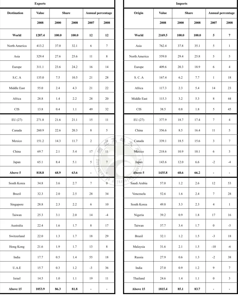
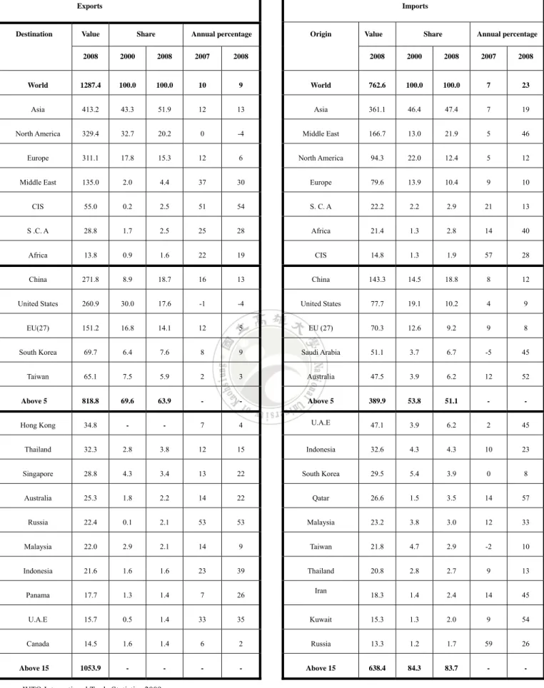
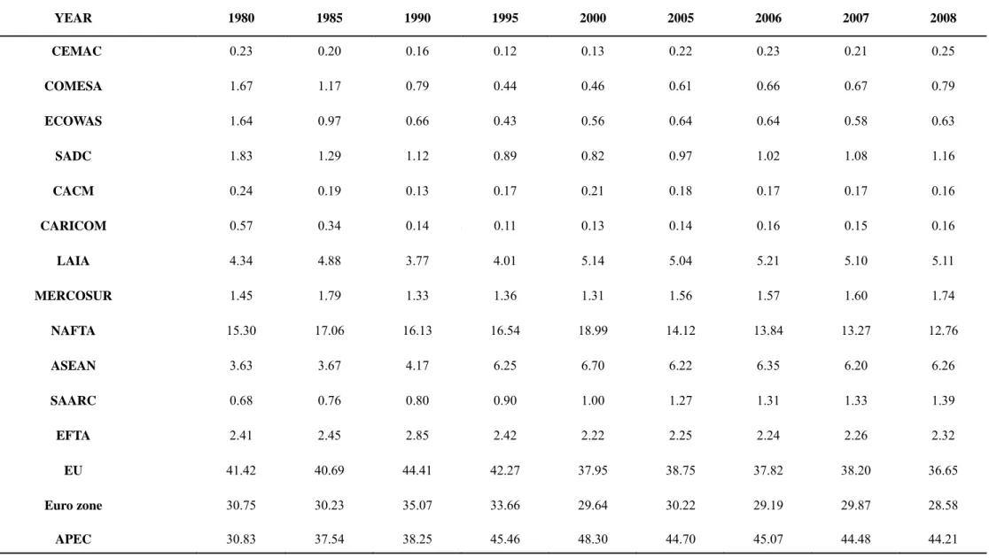
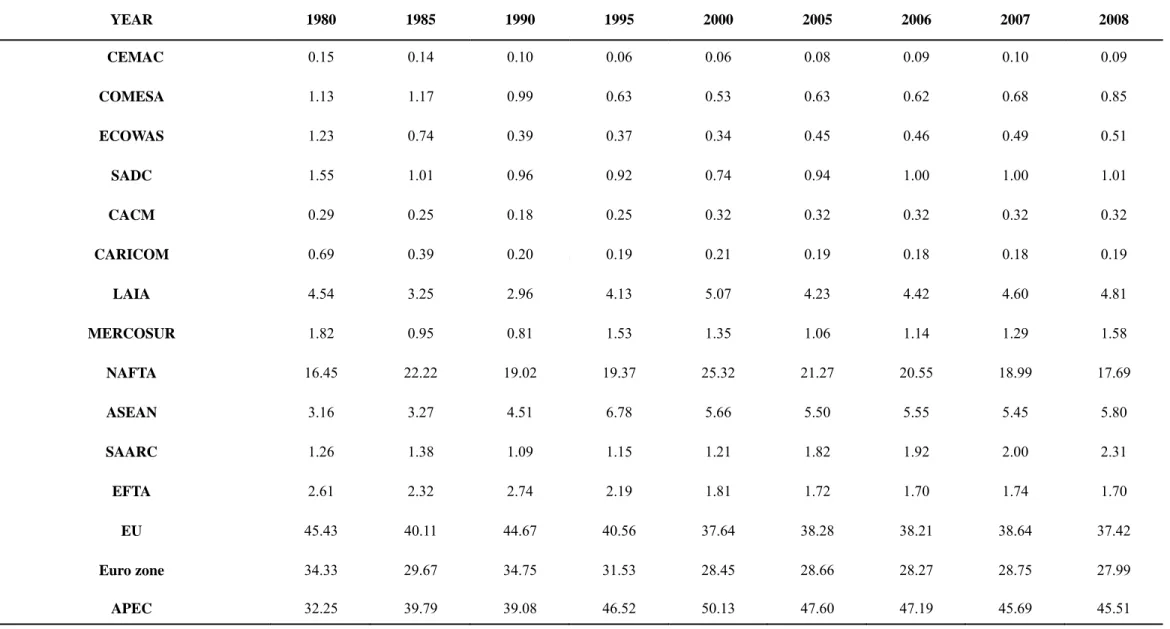
(15) highest in the world, followed by China with 8.9%. The United States and Japan also have large share of world merchandise trade in export and import, having more than 5% of world trade. As shown, the four countries play important roles in world merchandise trade, thus in the following, I briefly introduce each countries or organizations. In Table 4, merchandise export from the United States to North America is 413.2 in 2008. It also shows that merchandise import from Asia to the United States has also higher than other regions. As shown, from the United States to Israel has a relatively small share than other countries, but ranking the 15th. In contrast, import in merchandise trade from Thailand to the United States is relatively small, ranking the 15th. In Table 5, merchandise export from the European Union to Europe is 4313.5 in 2008. As shown, merchandise import from Europe to the European Union has also relatively high than other regions. As shown, from the European Union to Ukraine has relatively small share than other countries. Merchandise import from Canada to the European Union is relatively small, ranking the 15th. Table 6 shows the merchandise export from Japan to Asia is 406.2 in 2008. And Table 6 shows the merchandise import from Asia to Japan has also relatively higher than other regions. As shown, merchandise export from Japan to Canada has relatively small share than other countries. Merchandise import from Russian Federation to Japan is relatively small, ranking the 15th. The shares of exports and imports relative to the world trade have increased in some trade groups between year 1980 and year 2008. In Table 7 and 8, the shares of the European Union (EU) exports and imports are significantly higher than the other trade groups. As shown in Table 7, exports of the North American Free Trade Agreement (NAFTA) and Euro zone contribute to a large share of world exports, peaking to the highest in year 2000. During year 1980 to year 2008, the export share of the Asian Pacific Economic Cooperation (APEC) increased from 30.83 per cent in year 1980 to 9 .

(16) 44.21 per cent in year 2008. The shares of exports in the Association of South East Asian Nations (ASEAN) have also increased during the same period. In contrast, the export share of the Caribbean Community and Common Market (CARICOM) tends to be decreasing during the same period. With the exception of the Central American Common Market (CACM), CARICOM, NAFTA, APEC, the shares of imports in other trade groups in year 2008 are less than the shares of exports in the same year.. 10 .

(17) IV. The Empirical Models and Estimation Results 4.1. The empirical models In this section, I reconsider the various forms of the gravity models in the literature to analyze the determinants of bilateral trade flows. Typically, a simple gravity model assumes that the value of bilateral trade flows increases with economic sizes of trading countries, and decreases with their geographic distance. The gravity equation commonly used to study international trade flows takes the following form:6. ln. ln. ln. ln. ln. ln. ε. ,. (SGM). where Xijt is the value of exports from country i to country j in year t, Yit and Yjt are gross domestic products (GDPs) of the exporting and importing countries, Nit and Njt are the two country’s populations, DISTij is the distance between bilateral countries, LANGij is a dummy variable indicating if country i and country j use a common official language, ADJij is a dummy variable indicating that the two countries share a common border, and REIijt is a dummy variable assuming the value of 1 if the two countries join a trade bloc in year t and 0 otherwise, Rijt may include SIMILIARijt and other variables, and εijt is the residual term. To study the patterns of trade flows with various forms of gravity models, I use the pooled cross-section approach as the benchmark model. A three-way fixed effects model suggested by Mátyás (1997) with time-invariant variables is estimated for comparison. A specification of two-way fixed effects model with country-pair suggested by                                                              6. The standard gravity equation may include exporter’s and importer’s populations, or their per capita GDPs. 11 . .

(18) Freenstra (2002) and Cheng and Wall (2005) is also estimated. Finally, a generalized gravity model introduced by Egger and Pfaffermayr (2003) is re-estimated for comparison.. (1) The benchmark gravity model The benchmark model in the study is a pooled cross-section model that allows for the intercepts to differ over time. The simplest form of the pooled cross-section gravity model can be specified as:. ln. β ln. ln. ln. β ln. ln. ε ,. (PCS). where αt is the year-specific effect common to all trading countries. The other variables and dummies are defined in equation (SGM). The PCS model can be easily estimated by the OLS method.. (2) The three-way fixed effects model Since the benchmark model may suffer the heterogeneity problem, Mátyás (1997) develops three-way fixed effects model which a time dummy, two dummies of time-invariant, exporting and importing country effects are used. Mátyás (1998) also notes that the sample with large cross-section country specific effects should be treated as unobservable variables. In this study, a three-way FE model is constructed to consider two cases, with and without time-invariant variables. Equation (FE3-1) shows a three-way fixed effects model with time-invariant variables (i.e., distance, and language and adjacency dummies). Equation (FE3-2) shows the three-way fixed effects model without time-invariant variables for the comparison. They are:. 12 .

(19) ln. ln. ln. ln. ln. ln ln. ε , (FE3-1) ln. ln. ln. ln. ε ,. (FE3-2). where αt is the year-specific effect common to all trading pairs, αi and αj are country i and j country-specific effects, and the other variables and dummies are defined in equation (PCS).. (3) The two-way fixed effects model Freenstra (2002) and Cheng and Wall (2005) suggest a two-way fixed effects model in which the heterogeneity of various trading pairs is controlled for. The estimation specification can be written as:. ln. ln. ln. ln ε ,. ln (FE2). where αt is the year-specific effect common to all trading pairs, and αij is the specific country-pair effect indicating a pair of trading partners and common over all years. The other variables and dummies are defined in equation (PCS).. (4) The generalize fixed effects model Egger and Pfaffermayr (2003) use a generalized fixed effects model (FEG), which combine models FE3-2 and FE2, to estimate trade flows. The estimation can be specified as:. 13 .

(20) ln. ln. ln. ε ,. ln. ln (FEG). where the intercept constants and estimate parameters are defined as those model FE3 and FE2.. 4.2. The data The analysis in this section intends to identify the trend of the effects of trade flows with various gravity models. The study uses the F.O.B. values of bilateral exports as the dependent variable. The independent variables include exporting and importing countries’ real GDPs, populations, the distance between geographical centers of two trading countries, and the dummy variables to indicate if two countries’ official languages are the same, two countries share the same common border, and join the same trading bloc. Short descriptions of variables and data sources are provided in Table 9. The data set used in this study is a balanced panel with 52,486 observations. It widely covers countries at different levels of economic development and performance during the period 1986-2008. In each year, there are 2282 country trading pairs of 41 exporting and 57 importing countries. Table 10 demonstrates the list of the exporting and importing countries included in the study. To focus on the effect of regional blocs on bilateral trade, this study employs five regional bloc dummy variables, namely the European Union (EU), Euro area (EURO), North American Free Trade Agreement (NAFTA), ASEAN Free Trade Area (AFTA), and the South American Common Market (MERCOSUR). Descriptions of the each regional bloc’s year entered in force and its members are shown in Table 11. In this study, I assign a trading bloc dummy equal to one if two countries are acting. 14 .

(21) in a same trade bloc in a given year. Before 1992, there are 12 countries acting in the EU (see Table 11). After 2004, eight countries of central and eastern European countries join the EU, including Czech Republic, Estonia, Latvia, Lithuania, Hungary, Poland, Slovenia and Slovakia. Then, Bulgaria and Romania joined the EU in 2007. In this study, the EU dummy is set to be one when two countries are acting in the EU in year t. The Euro area is a currency union that people use the Euro instead of their earlier official currencies. After EURO goes into effect in 1999, there are 16 EU countries joining the economic and monetary union during 1999-2009. In 1999, Austria, Belgium, Finland, France, Germany, Ireland, Italy, Luxembourg, the Netherlands, Portugal and Spain have decided to use the Euro as their official currency. Greece became one of EURO member countries in 2001. Slovenia adopted the euro as the official currency in 2007, Cyprus and Malta in 2008, and Slovakia in 2009. To consider the monetary effect of the EU on trade flows, this study uses a dummy to indicate if two countries are using the Euro in year t. The Canada-US Free Trade Agreement (CUFTA) was formed in 1989. Then, the agreement was extended to include Mexico after the North American Free Trade Agreement entered into effect in 1994. To estimate this effect, this study let a dummy be the value of one for bilateral trade between the United States and Canada in 1989-1993, and the trade between Mexico, the United States and Canada during 1994-2008. The Association of Southeast Asian Nations (ASEAN) was established in 1967 by the five original member countries, including Indonesia, Malaysia, the Philippines, Singapore, and Thailand. Brunei Darussalam became the sixth member of the ASEAN in 1984, and Vietnam in 1995, Laos and Myanmar in 1997, and Cambodia became the ASEAN member in 1999. Subsequently, the ASEAN Free Trade Area (AFTA) was formed to liberalize trade among the ASEAN countries which went into force in 2002. To estimate the effect, the study uses the AFTA dummy taking the value of one for 15 .

(22) bilateral trade between the ten members during 2002-2008. The MERCOSUR was created by four South American countries (Argentina, Brazil, Paraguay and Uruguay) in 1994, and then Venezuela joined it in 2006. To estimate the effect, I use the MERCOSUR dummy by setting the value of one between Argentina, Brazil, Paraguay and Uruguay for 1994-2006, and between Argentina, Brazil, Paraguay, Uruguay and Venezuela for 2006-2008. To control for different levels of economic performance, this study uses dummies to indicate if a trading pair is developed or developing country in a given year. According to the CIA’s The World Factbook 2009, a country is defined as a developed country (a high-income economy) if it’s gross national income (GNI) in year 2005 was higher than and equal to $10,726, otherwise denoted as a developing country. Table 12 shows the developed and developing countries. Some Africa countries may be due to suffer the wars, we exclude some dummy variables of data. They are twenty-four developed countries in the data set, namely Australia, Austria, Canada, Denmark, Finland, France, Germany, Greece, Hong Kong, Iceland, Ireland, Italy, Japan, Korea, the Netherlands, New Zealand, Norway, Portugal, Singapore, Spain, Sweden, Switzerland, the United Kingdom, and the United States.. 4.3. Main estimation results In this section, I will estimate the gravity models above, including the benchmark gravity, three-way fixed effects, two-way fixed effects, and generalize fixed effects models. Table 13 shows the main estimation results. Column one presents the result of the PCS model, columns two and three present the results of three-way effect model with time-invariant, and without time-invariant respectively, and column four shows for the two-way fixed effect model, and the last column the FEG model. Table 13 also 16 .

(23) provides the adjusted R2 (commonly as the empirical power), and the information criteria AIC and SIC (to indicate an appropriate model with the smallest value). According to the result in the first column of Table 13, a 10% rise in exporter’s GDP should be associated with a 11.7% rise in exports. If an importer’s GDP rises by 10%, exports should rise by 7.95%. Holding the other condition to be the same, if an exporter’s population rises by 10%, exports should decrease by 0.66%, while an importer’s population increases by 10%, its exports should increase 1.04%. Also as shown in column one of Table 13, a country will export 88.6% less to a market that is double as distant as another identical market. Exports would be higher by 74.8% than the other trade flows if trading partners use the same language, while exports should be higher by 28.7% if trading partners share a common border. Trade bloc dummy variables are used to evaluate the effect of free trade agreements. In column one of Table 13, the coefficient on AFTAijt and MERCOSURijt are positive and significant statistically, indicating that bilateral trade in the AFTAijt and MERCOSURijt countries is more intense than the other countries. In contrast, for the EUijt, the PCS model predicts a -60.8% lower of bilateral trade if both exporting and importing countries are the EUijt members. The PCS model also indicates that intra-EURO trade is about 11.6% higher than the average trade flow, but the effect is statistically insignificant. Intra-NAFTA trade is about -13.2% lower than the average trade flow, and statistically significant. The second column of Table 13 reports the estimation result for the three-way fixed model with time-invariant variables. According the result, a 10% rise in exporter’s GDP should be associated with a 13.16% rise in exports. If an importer’s GDP rises by 10%, exports should rise by 12.78%. Holding the other condition to be the same, if an exporter’s population rises by 10%, exports should increase by 0.9%, while an importer’s population increases by 10%, its exports should increase 0.9%. Also as shown in column two of Table 13, a country will export 130% less to a market that is 17 .

(24) double as distant as another identical market. Exports would be higher by 76.5% than the other trade flows if trading partners use the same language, while exports should be lower by 28% if trading partners share a common border. Column two of Table 13 indicates that the coefficient on NAFTAijt and MERCOSURijt are positive and significant statistically, i.e., bilateral trade flows in the NAFTAijt and MERCOSURijt countries are more intense than the other countries. In contrast, for the EUijt, the three-way fixed model predicts a -43% lower of bilateral trade if both exporting and importing countries are the EUijt members. The three-way fixed model also indicates that intra-EURO trade is about 12.8% higher than the average trade flow, and intra-AFTA trade is about 6.6% higher than the average trade flow, and statistically. However, both of their effects are statistically insignificant. The third column of Table 13 reports the estimation result for three-way fixed effects model without time-invariant. Specifically, it suggests that acting in EUijt tends to an increase in trade of 100.1%, and that NAFTAijt and AFTAijt led to increase in trade of greater than 200%, and that MERCOSURijt causes members to trade greater than 400% than an average trade. The estimated effect of the NAFTAijt using the three-way fixed effects model without time-invariant indicates that there is something special about the relationship between Mexico, the United States and Canada that makes them trade relatively less with each other than the gravity variables would predict. The fourth column of Table 13 reports the estimation result for model FE2. As shown in the result, a 10% rise in exporter’s GDP should be associated with a 12.9% rise in exports. If an importer’s GDP rises by 10%, exports should rise by 12.48%. Holding the other conditions to be the same, if an exporter’s population rises by 10%, exports should increase by 1.59%, while an importer’s population increases by 10%, and its exports should increase 3.54%. With regarding the REI effect on trade flows, the coefficients on NAFTAijt and MERCOSURijt are positive and significant statistically. In 18 .

(25) contrast, the coefficients on EUijt and AFTAijt are statistically insignificant. The last column of Table 13 reports the estimation results for the FEG model. According to the result, a 10% rise in exporter’s GDP should be associated with a 12.9% rise in exports. If an importer’s GDP rises by 10%, exports should rise by 12.48%. Holding the other condition to be the same, if an exporter’s population rises by 10%, exports should increase by 1.59%, while an importer’s population increases by 10%, its exports should increase 3.54%. The REA coefficients on bilateral trade are the same as those of model FE2. According to the estimation result, models FE 2 and FEG have high explanatory power of the adjusted R2. Also, from the estimation result, models FE2 and FEG are identical, except for the dummy variables which indicate specific trading pairs and trading countries. Based on information criterion BIC, model FE2 is preferred.. 4.4. The results of a further study on country-specific effects In this subsection, I intend to discuss the estimation difference between the estimated results of the exporter-specific (αi) and importer-specific (αj) country dummies, and country-pair (αij) specific dummies. The year dummies indicating the economic cycle, which are common to all trading countries and trading-pairs, are omitted here. Table 14 summarizes the main results of these dummies for comparison, including four regional blocs, AFTA, EU, MERCUSOR, and NAFTA. As noted above, αi and αj denote the country-specific effects of exporting and importing countries respective. Thus, the sum of αi and αj indicates how much the exports from country i to country j are more intensive than an average trading-pair. The last column in Table 14 shows of the country-pair effect αij estimated by using model FE2 is higher than estimated (αi +αj) by using model FE3. As noted in Table 13, models. 19 .

(26) FE2 and FEG are better specifications. That is, it implies a trading-pair flow is underestimated with model FE3 if αij is higher than (αi +αj). As shown in Table 14, αij is greater than (αi +αj) for each country-pair trading flow between AFTA’s member countries, indicating that model FE2 predicts more intensive trade between them, and that with model FE3 country-specific trader effects may be underestimated. Note that bilateral trade flows between Singapore and its AFTA partner countries are particularly more intensive than an average trading-pair trade. The results in Table 14 also reveal that each trading flow between MERCUSOR’s member countries is also significantly more intensive than an average trading-pair when model FE2 is adopted. In North America, trade between Mexico and its partners Canada and USA is more intensive. By contrast, the results for EU member show ambiguous, i.e. whether αij is not always greater or less than (αi +αj). Roughly judging by the calculation results, bilateral trade flows from Austria to Germany, from Italy to Austria, from Netherlands to Demark, from UK to Ireland, bilateral trade between Spain and Portugal, and trade within Demark, Finland and Sweden, are shown to be more intensive with model FE2.This may imply that the estimation using model FE3 may underestimate less-distant bilateral trade flows.. 20 .

(27) VI. The conclusions This dissertation is to estimate bilateral trade flows by using the gravity model in which bilateral trade flows. Bilateral trade flows explain that trade flows are expected to increase in the size of two trading partner countries, and decrease in the cost of transportation between them. To estimate trade flows, I use the most popular approach in which a dummy variable is used to identify regional economic integration (REI), and the standard way of assessing such trading agreements is to include dummy variables indicating a common grouping into the gravity models. To explain the trade bloc effects on within-regional trade, I use one dummy variable for each regional bloc, including for the EU, NAFTA, AFTA and MERCOSUR. By using the conventional gravity model PCS, which does not control for trading-pair heterogeneity, the estimated coefficients of the EURO are negative. That is, if countries join these blocs, bilateral trade tends to be less intensive. In contrast, with the fixed effects models the study obtains a positive coefficient of the EU and EURO. The coefficients estimated by the PCS and FE3 models on NAFTA, AFTA and MERCOSUR are positive and significant statistically. This means that intra-bloc trade is higher than an average trade for these trading blocs. Holding all else constant, the estimated coefficients on the changes of developed exporter’s and developed importer’s GDPs are positive and significant statistically, and a developed exporter will send lower of exports to a market that is twice as distant as another otherwise-identical market, and higher to a country that uses the same language and shares a common border. From the estimation result of the PCS model, the coefficients on the changes of developed exporter’s and importer’s GDPs are significantly positive, indicating that, although faster growing countries do trade more, the increase is more than proportionate. As these models, exports tend to be. 21 .

(28) capital-intensive as indicated by the positive and greater than unity. Holding all else constant, the estimation coefficients on IIT of these models predicts that bilateral trade increase with higher IIT level. In the study, using dummy variables to control for the country-pair heterogeneity may involve a large number of parameters in the gravity model. I use the statistics of information criteria (AIC or BIC) to detect if the fixed effects model is over parameterized, and to select a better specification for the study of trade flows. Regarding to the choice between the various gravity models, based on information criterion BIC, model FE2 is preferred in this study. In order to get more information from the study of bilateral trade flows, future research may focus on the determination of bilateral industry trade across countries.. 22 .

(29) References Aitken, N. D., (1973) “The Effect of the EEC and EFTA on European Trade: A Temporal Cross-section Analysis,” American Economic Review, 63, 881-892. Anderson, J. E., (1979) “A Theoretical Foundation for the Gravity Equation,” American Economic Review, 69, 1, 106-116. Abrams, R. K., (1980) “International Trade Flows under Flexible Exchanges Rates,” Federal Reserve Bank of Kansas City, Economic Review, 65, 3, 3-10. Anderson, J. E. and van Wincoop, E., (2003) “Gravity with Gravitas: A Solution to the Border Puzzle,” American Economic Review, 93, 1, 170-192. Baier, S. L. and Bergstrand, J. H., (2001) “The Growth of World Trade: Tariffs, Transport Costs, and Income Similarity,” Journal of International Economics, 53, 1, 1-27. Baier, S. L. and Bergstrand, J. H., (2007) “Do Free Trade Agreements Actually Increase Members’ International Trade? ” Journal of International Economics, 71, 72-95. Baier, S. L. and Bergstrand, J. H., (2009) “Estimating the Effects of Free Trade Agreement on International Trade Flows Using Matching Econometrics” Journal of International Economics, 77, 63-76. Bayoumi, T. and Eichengreen, B., (1997) “Is Regionalism Simply a Diversion? Evidence from the Evolution of the EC and EFTA,” in Regionalism versus Multilateral Trade Arrangements, T. Ito and A.O. Krueger, Eds., University of Chicago Press, Chicago. Bergstrand, J. H., (1985) “The Gravity Equation in International Trade: Some Microeconomic Foundations and Empirical Evidence,” Review of Economics and Statistics, 67, 474-481. Bergstrand, J. H., (1989) “The Generalized Gravity Equation, Monopolistic Competition, and the Factor-Proportions: Theory of International Trade,” Review of Economics and Statistics, 71, 143-153.. 23 .

(30) Brada, J. C. and Mendez, J. A., (1983) “Regional Economic Integration and the Volume of Intra- Regional Trade: A Comparison of Developed and Developing Country Experience,” Kyklos, 36, 589-603. Brada, J. C. and J. A. Mendez, (1985) “Economic Integration among Developed, Developing and Centrally Planned Economies: A Comparative Analysis,” Review of Economics and Statistics, 67, 4, 549-556. Boisso, D. and Ferrantino, M., (1997), “Economic Distance, Cultural Distance, and Openness in International Trade: Empirical Puzzles,” Journal of Economic Integration, 12, 456-484. Cheng, I. H. and Wall, H. J., (2005) “Controlling for Trading-pair Heterogeneity in Gravity Models of Trade and Integration,” The Federal Reserve Bank of St. Louis Review, 87, 1, 49-63. Cheng, I. H. and Tsai, Y. Y., (2008) “Estimating the Staged Effects of Regional Economic Integration on Trade Volumes,” Applied Economics, 40,383-393. Deardorff, A.V., (1998) “Determinants of Bilateral Trade: Does Gravity Work in a Neoclassical World?” in J. A. Frankel, Ed., The Regionalization of the World Economy, University of Chicago Press. Egger, P., (2000) “A Note on the Proper Econometric Specification of the Gravity Equation,” Economics Letters, 66, 25-31. Egger, P., (2004) “Estimating Regional Trading Block Effects with Panel Data,” Review of World Economics, 140, 1, 151-166. Egger, P. and Larch, M., (2008) “Interdependent Preferential Trade Agreement Memberships: An Empirical Analysis,” Journal of International Economics, 76, 384-399. Egger, P., and Pfaffermayr, M., (2003) “The Proper Panel Econometric Specification of the Gravity Equation: A Three-way Model with Bilateral Interaction Effects,” Empirical Economics,” 28, 3, 571-580. Egger, H., Egger, P. and Greenaway, D., (2008) “The Trade Structure Effects of Endogenous Regional Trade Agreements,” Journal of International Economics, 74, 24 .

(31) 278-298. Eichengreen, B. and Irwin, D. A., (1998) “The Role of History in Bilateral Trade Flows,” in J. A. Frankel, Ed., The Regionalization of the World Economy, University of Chicago Press. Frankel, F., Stein, E. and Wei, S., (1995) “Trading Blocs and Americas: The Natural, the Unnatural, and the Super-natural,” Journal of Development Economics, 47, 61-95. Hsieh, Y.W., (2009), On the Study of the Determination of Bilateral Trade Flows, Unpublished MA Dissertation, University of Kaohsiung, Kaohsiung, Taiwan. Krugman, P., (1991) “The Move to Free Trade Zones,” in Policy Implications of Trade and Currency Zones, Federal Reserve Bank of Kansas City, 7-41. Krishna, P., (2005) “Trade blocs: Economics and Politics,” Cambridge University Press. Linnemann, H., (1966) “An Econometric Study of International Trade Flows,” North-Holland Publishing Company, Amsterdam. Mátyás, L., (1997) “Proper Econometric Specification of the Gravity Model,” The World Economy, 20, 363-368. Mátyás, L., (1998) “The Gravity Model: Some Econometric Consideration,” The World Economy, 20, 3, 397-401. Magee, S. P., (2008) “New Measures of Trade Creation and Trade Diversion,” Journal of International Economic, 75, 349-362. Oguledo, V. I. and MacPhee, C. R., (1994) “Gravity Model: A Reformulation and an Application to Discriminatory Trade Arrangements,” Applied Economics, 26, 107-120. Pöyhönen, P., (1963) “A Tentative Model for the Volume of Trade Between Countries,” The Weltwirtschaftliches Archive, 90, 93-100. Sapir, A., (1997) “Domino Effects in West European Trade,” CEPR Discussion Paper 1576.. 25 .

(32) Sawyer, W. C., and Sprinkle, R. L., (1997) “The Demand for Imports and Exports in Japan: A Survey,” Journal of the Japanese and International Economies, 11, 2, 247-59. Summers, L., (1991) “Regionalism and the World Trading System,” in Policy Implications of Trade and Currency Zones, Federal Reserve Bank of Kansas City. Subramanian, A. and Wei, S. J., (2007), “The WTO Promotes Trade, Strongly but Unevenly,”Journal of International Economic, 72, 151-175. Tinbergen, J., (1962) Shaping the World Economy: Suggestions for an International Economic Policy, The Twentieth Century Fund, New York. Viner, J., (1950) “The Economics of Customs Unions,” The Customs Union Issue, Carnegie Endowment for International Peace, New York. Winters, L. A., (1992) “Bilateral Trade Elasticities for Exploring the Effects of ‘1992’,” in L. A. Winters, Ed., Trade Flows and Trade Policy after ‘1992’, The Cambridge University Press. Wonnacott, P. and Lutz, M., (1987) “Is There a Case for Free Trade Areas?” in Jeffrey Schott, Ed., Free Trade Areas and U.S. Trade Policy, Institute for International Economics, Washington, DC.. 26 .

(33) Table 1.. The total value of exports in different geographical regions Unit: Millions of dollars (Percentage) YEAR. 1980. 1990. 2000. 2005. 2006. 2007. 2008. 121,876. 110,670. 152,143. 311,585. 372,088. 429,089. 553,177. (2.99%). (3.18%). (2.36%). (2.97%). (3.07%). (3.07%). (3.45%). 111,352. 143,808. 364,468. 573,473. 686,022. 769,679. 885,097. (5.47%). (4.13%). (5.65%). (5.47%). (5.66%). (5.52%). (5.52%). 76,165. 280,565. 774,898. 1,538,367. 1,846,744. 2,186,288. 2,475,315. (3.74%). (8.05%). (12.02%). (14.67%). (15.23%). (15.67%). (15.45%). 73,957. 145,284. 431,944. 652,732. 770,6567. 864,964. 1,003,790. (3.63%). (4.17%). (6.70%). (6.22%). (6.35%). (6.20%). (6.26%). 293,549. 521,758. 1,058,871. 1,267,052. 1,428,252. 1,580,115. 1,753,793. (14.43%). (14.98%). (16.42%). (12.08%). (11.78%). (11.32%). (10.94%). 135,979. 299,157. 510,653. 637,675. 696,720. 754,603. 847,255. (6.68%). (8.59%). (7.92%). (6.08%). (5.74%). (5.41%). (5.29%). 892,271. 1,647,000. 2,591,769. 4,300,946. 4,860,295. 5,647,561. 6,247,494. (43.85%). (47.28%). (40.19%). (41.01%). (40.07%). (40.46%). (38.98%). Developing economies Africa. America. Eastern Asia. South-Eastern Asia. Developed economies America. Asia. Europe. Sources: UNCTAD Handbook of Statistics 2009, UN Yearbook of International Trade Statistics. Note: Exports are calculated in F.O.B. unit and measured in millions of dollars. The shares of exports relative to the world trade in different regions are in parentheses. 27 .

(34) Table 2.. The total value of imports in different geographical regions Unit: Millions of dollars (Percentage) YEAR. 1980. 1990. 2000. 2005. 2006. 2007. 96,856. 101,718. 132,878. (4.66%). (2.83%). 123,594. 2008. 267,242. 312,189. 378,503. 482,155. (1.99%). (2.48%). (2.52%). (2.66%). (2.95%). 127,275. 392,134. 531,709. 633,841. 753,712. 902,341. (5.95%). (3.54%). (5.89%). (4.93%). (5.12%). (5.30%). (5.52%). 85,536. 265,896. 742,868. 1,411,111. 1,647,693. 1,910,483. 2,210,617. (4.12%). (7.40%). (11.15%). (13.07%). (13.30%). (13.43%). (13.53%). 65,641. 162,292. 377,441. 594,318. 687,976. 776,356. 948,366. (3.16%). (4.51%). (5.67%). (5.51%). (5.55%). (5.46%). (5.80%). 320,210. 641,358. 1,505,270. 2,065,550. 2,278,836. 2,408,102. 2,584,666. (15.42%). (17.84%). (22.59%). (19.14%). (18.40%). (19.92%). (15.82%). 151,080. 252,162. 417,197. 562,064. 629,908. 678,868. 830,248. (7.27%). (7.01%). (6.26%). (5.21%). (5.09%). (4.77%). (5.08%). 998,105. 1,705,494. 2,630,452. 4,320,581. 4,947,006. 5,750,000. 6,396,748. (48.06%). (47.44%). (39.48%). (40.03%). (39.93%). (40.41%). (39.15%). Developing economies Africa. America. Eastern Asia. South-Eastern Asia. Developed economies America. Asia. Europe. Sources: UNCTAD Handbook of Statistics 2009, UN Yearbook of International Trade Statistics. Note: Imports are calculated in C.I.F. unit and measured in millions of dollars. The shares of imports relative to the world trade in different regions are in parentheses. 28 .

(35) Table 3.. Leading exporters and importers in world merchandise trade, 2008 Unit: Billions of dollars and percentage. Rank. Exporters. Value. Share. Annual percentage. Rank. Importers. Value. Share. change. change. 1. Germany. 1461.9. 9.1. 11. 1. United States. 2169.5. 13.2. 7. 2. China. 1428.3. 8.9. 17. 2. Germany. 1203.8. 7.3. 14. 3. United States. 1287.4. 8.0. 12. 3. China. 1132.5. 6.9. 18. 4. Japan. 782.0. 4.9. 9. 4. Japan. 762.6. 4.6. 23. 5. Netherlands. 633.0. 3.9. 15. 5. France. 705.6. 4.3. 14. 6. France. 605.4. 3.8. 10. 6. United Kingdom. 632.0. 3.8. 1. 7. Italy. 538.0. 3.3. 8. 7. Netherlands. 573.2. 3.5. 16. 8. Belgium. 475.6. 3.0. 10. 8. Italy. 554.9. 3.4. 8. 9. Russia. 471.6. 2.9. 33. 9. Belgium. 469.5. 2.9. 14. 10. United Kingdom. 458.6. 2.9. 4. 10. Korea,South. 435.3. 2.7. 22. 11. Canada. 456.5. 2.8. 9. 11. Canada. 418.3. 2.5. 7. 12. Korea,South. 422.0. 2.6. 14. 12. Spain. 401.4. 2.4. 3. 13. Hong Kong. 370.2. 2.3. 6. 13. Hong Kong. 393.0. 2.4. 6. 14. Singapore. 338.2. 2.1. 13. 14. Mexico a. 323.2. 2.0. 9. 15. Saudi Arabia. 313.4. 2.0. 33. 15. Singapore. 319.78. 1.947. 22. 16. Mexico. 291.7. 1.8. 7. 16. India. 293.4. 1.8. 35. 17. Spain. 268.3. 1.7. 6. 17. Russia. 291.9. 1.8. 31. 18. Taiwan. 255.6. 1.6. 4. 18. Taiwan. 240.4. 1.5. 10. 19. U.A.E. b. 231.6. 1.4. 28. 19. Poland. 204.3. 1.2. 23. 20. Switzerland. 200.3. 1.2. 16. 20. Turkey. 202.0. 1.2. 19. 21. Malaysia. 199.5. 1.2. 13. 21. Australia. 200.3. 1.2. 21. 22. Brazil. 197.9. 1.2. 23. 22. Austria. 183.4. 1.1. 13. 23. Australia. 187.3. 1.2. 32. 23. Switzerland. 183.2. 1.1. 14. 24. Sweden. 183.4. 1.1. 9. 24. Brazil. 182.4. 1.1. 44. 25. Austria. 181.0. 1.1. 11. 25. Thailand. 178.7. 1.1. 28. 26. Thailand. 177.8. 1.1. 17. 26. Sweden. 27. India. 177.5. 1.1. 21. 28. Norway. 172.5. 1.1. 29. Poland. 168.0. 30. Czech Republic.. a. 167.2. 1.0. 10. 27. U.A. E.. b. 165.6. 1.0. 25. 27. 28. Malaysia. 156.9. 1.0. 7. 1.0. 20. 29. Czech Republic a. 141.5. 0.9. 20. 146.3. 0.9. 19. 30. Indonesia. 126.2. 0.8. 36. Total of above. 13080..8. 81.5. -. Total of above. 13411.8. 81.6. -. World. 16070.0. 100.0. 15. 16422.0. 100.0. 15. World. Source: WTO International Trade Statistics 2009 Note: a-Imports are valued f.o.b., b- Secretariat estimates, c- Includes significant re-exports or imports for re-export.. 29 . Annual percentage.

(36) Table 4. Merchandise trade of the United States by origin and destination, 2008 Unit: Billions of dollars and percentage Exports Destination. Imports. Value. Share. Annual percentage. 2008. 2000. 2008. 2007. 2008. World. 1287.4. 100.0. 100.0. 12. 12. North America. 413.2. 37.0. 32.1. 6. Asia. 329.4. 27.6. 25.6. Europe. 311.1. 23.6. S.C. A. 135.0. Middle East. Origin. Share. Annual percentage. 2008. 2000. 2008. 2007. 2008. World. 2169.5. 100.0. 100.0. 5. 7. 7. Asia. 762.4. 37.8. 35.1. 5. 1. 11. 8. North America. 559.0. 29.4. 25.8. 5. 5. 24.2. 16. 14. Europe. 409.6. 20.3. 18.9. 6. 4. 7.5. 10.5. 21. 28. S. C. A. 167.4. 6.2. 7.7. 1. 18. 55.0. 2.4. 4.3. 21. 22. Africa. 117.3. 2.3. 5.4. 14. 23. Africa. 28.8. 1.4. 2.2. 28. 20. Middle East. 115.3. 3.2. 5.3. 8. 44. CIS. 13.8. 0.4. 1.1. 49. 32. CIS. 38.5. 0.8. 1.8. 5. 45. EU (27). 271.8. 21.6. 21.1. 15. 11. EU (27). 377.9. 18.7. 17.4. 7. 4. Canada. 260.9. 22.6. 20.3. 8. 5. China. 356.6. 8.5. 16.4. 11. 5. Mexico. 151.2. 14.3. 11.7. 2. 11. Canada. 339.1. 18.5. 15.6. 3. 7. China. 69.7. 2.1. 5.4. 17. 11. Mexico. 218.6. 10.9. 10.1. 6. 3. Japan. 65.1. 8.4. 5.1. 5. 7. Japan. 143.6. 12.0. 6.6. -2. -4. Above 5. 818.8. 68.9. 63.6. -. -. Above 5. 1435.8. 68.6. 66.2. -. -. South Korea. 34.8. 3.6. 2.7. 7. 0. Saudi Arabia. 57.0. 1.2. 2.6. 12. 53. Brazil. 32.3. 2.0. 2.5. 28. 34. Venezuela. 52.6. 1.6. 2.4. 7. 28. Singapore. 28.8. 2.3. 2.2. 6. 10. South Korea. 49.8. 3.3. 2.3. 4. 1. Taiwan. 25.3. 3.1. 2.0. 14. -4. Nigeria. 39.2. 0.9. 1.8. 17. 16. Australia. 22.4. 1.6. 1.7. 8. 17. Taiwan. 37.7. 3.4. 1.7. 0. -5. Switzerland. 22.0. 1.3. 1.7. 18. 29. Brazil. 32.1. 1.2. 1.5. -3. 18. Hong Kong. 21.6. 1.9. 1.7. 13. 8. Malaysia. 31.6. 2.1. 1.5. -10. -6. India. 17.7. 0.5. 1.4. 55. 18. Russia. 27.9. 0.6. 1.3. -2. 38. U.A.E. 15.7. 0.3. 1.2. -3. 36. India. 27.0. 0.9. 1.2. 9. 7. Israel. 14.5. 1.0. 1.1. 19. 11. Thailand. 24.6. 1.4. 1.1. 0. 3. 1053.9. 86.3. 81.8. -. -. Above 15. 1815.4. 85.1. 83.7. -. -. Above 15. Source: WTO International Trade Statistics 2009.. 30 . Value.

(37) Table 5. Merchandise trade of the European Union (27) by origin and destination, 2008 Unit: Billions of dollars and percentage Exports Destination. Imports. Value. Share. Annual percentage. 2008. 2000. 2008. 2007. 2008. World. 1287.4. 5898.4. 100.0. 16. 10. Europe. 413.2. 4313.5. 73.1. 16. Asia. 329.4. 440.5. 7.5. North America. 311.1. 434.7. CIS. 135.0. Africa. Origin. Share. Annual percentage. 2008. 2000. 2008. 2007. 2008. World. 6255.8. 100.0. 100.0. 16. 12. 9. Europe. 4298.9. 69.2. 68.7. 16. 10. 17. 11. Asia. 784.5. 12.0. 12.5. 19. 9. 7.4. 7. 4. CIS. 329.5. 2.7. 5.3. 12. 31. 218.3. 3.7. 33. 25. North America. 323.7. 8.3. 5.2. 15. 9. 55.0. 171.8. 2.9. 22. 24. Africa. 214.2. 2.9. 3.4. 12. 30. Middle East. 28.8. 156.1. 2.6. 17. 18. S.C.A. 128.6. 1.7. 2.1. 17. 17. S.C.A. 13.8. 89.0. 1.5. 21. 20. Middle East. 111.0. 1.9. 1.8. 7. 19. EU(27). 271.8. 68.0. 67.4. 16. 9. EU (27). 3973.5. 64.5. 63.5. 16. 9. United States. 260.9. 8.9. 6.1. 6. 2. China. 363.7. 2.7. 5.8. 30. 15. Russia. 151.2. 0.8. 2.6. 34. 27. United States. 268.3. 7.3. 4.3. 13. 8. Switzerland. 69.7. 2.7. 2.4. 15. 13. Russia. 254.0. 2.2. 4.1. 11. 28. China. 65.1. 1.0. 1.9. 23. 17. Norway. 135.3. 1.7. 2.2. 6. 29. Above 5. 818.8. 81.4. 80.5. -. -. Above 5. 4994.7. 78.4. 79.8. -. -. Turkey. 34.8. 1.2. 1.4. 15. 11. Switzerland. 117.8. 2.2. 1.9. 17. 12. Norway. 32.3. 1.0. 1.1. 24. 8. Japan. 109.9. 3.3. 1.8. 11. 2. Japan. 28.8. 1.7. 1.0. 6. 3. Turkey. 67.5. 0.7. 1.1. 23. 5. U.A.E. 25.3. 0.5. 0.8. 16. 27. South Korea. 57.9. 1.0. 0.9. 11. 2. India. 22.4. 0.5. 0.8. 32. 15. Brazil. 52.1. 0.7. 0.8. 31. 16. Canada. 22.0. 0.8. 0.7. 6. 8. 50.3. 0.5. 0.8. 15. 34. South Korea. 21.6. 0.6. 0.6. 18. 11. India. 43.2. 0.5. 0.7. 28. 19. Brazil. 17.7. 0.6. 0.6. 30. 32. Algeria. 41.7. 0.6. 0.7. -7. 48. Australia. 15.7. 0.6. 0.6. 17. 19. Taiwan. 35.4. 1.0. 0.6. 6. -1. Ukraine. 14.5. 0.2. 0.6. 34. 21. Canada. 35.0. 0.7. 0.6. 29. 10. 1053.9. 89.1. 88.7. -. -. Above 15. 5605.5. 89.4. 89.6. -. -. Above 15. Libya. Source: WTO International Trade Statistics 2009.. . Note: Figures are affected by the "INTRASTAT" system of recording trade between EU member states. . 31 . Value.

(38) Table 6. Merchandise trade of Japan by origin and destination, 2008 Unit: Billions of dollars and percentage Exports. Destination. Imports. Value. Share. Annual percentage. 2008. 2000. 2008. 2007. 2008. World. 1287.4. 100.0. 100.0. 10. 9. Asia. 413.2. 43.3. 51.9. 12. North America. 329.4. 32.7. 20.2. Europe. 311.1. 17.8. Middle East. 135.0. CIS. Origin. Value. Annual percentage. 2008. 2000. 2008. 2007. 2008. World. 762.6. 100.0. 100.0. 7. 23. 13. Asia. 361.1. 46.4. 47.4. 7. 19. 0. -4. Middle East. 166.7. 13.0. 21.9. 5. 46. 15.3. 12. 6. North America. 94.3. 22.0. 12.4. 5. 12. 2.0. 4.4. 37. 30. Europe. 79.6. 13.9. 10.4. 9. 10. 55.0. 0.2. 2.5. 51. 54. S. C. A. 22.2. 2.2. 2.9. 21. 13. S .C. A. 28.8. 1.7. 2.5. 25. 28. Africa. 21.4. 1.3. 2.8. 14. 40. Africa. 13.8. 0.9. 1.6. 22. 19. CIS. 14.8. 1.3. 1.9. 57. 28. China. 271.8. 8.9. 18.7. 16. 13. China. 143.3. 14.5. 18.8. 8. 12. United States. 260.9. 30.0. 17.6. -1. -4. United States. 77.7. 19.1. 10.2. 4. 9. EU(27). 151.2. 16.8. 14.1. 12. 5. EU (27). 70.3. 12.6. 9.2. 9. 8. South Korea. 69.7. 6.4. 7.6. 8. 9. Saudi Arabia. 51.1. 3.7. 6.7. -5. 45. Taiwan. 65.1. 7.5. 5.9. 2. 3. Australia. 47.5. 3.9. 6.2. 12. 52. Above 5. 818.8. 69.6. 63.9. -. -. Above 5. 389.9. 53.8. 51.1. -. -. Hong Kong. 34.8. -. -. 7. 4. U.A.E. 47.1. 3.9. 6.2. 2. 45. Thailand. 32.3. 2.8. 3.8. 12. 15. Indonesia. 32.6. 4.3. 4.3. 10. 23. Singapore. 28.8. 4.3. 3.4. 13. 22. South Korea. 29.5. 5.4. 3.9. 0. 8. Australia. 25.3. 1.8. 2.2. 14. 22. Qatar. 26.6. 1.5. 3.5. 14. 57. Russia. 22.4. 0.1. 2.1. 53. 53. Malaysia. 23.2. 3.8. 3.0. 12. 33. Malaysia. 22.0. 2.9. 2.1. 14. 9. Taiwan. 21.8. 4.7. 2.9. -2. 10. Indonesia. 21.6. 1.6. 1.6. 23. 39. Thailand. 20.8. 2.8. 2.7. 9. 13. Panama. 17.7. 1.3. 1.4. 7. 26. 18.3. 1.4. 2.4. 14. 45. U.A.E. 15.7. 0.5. 1.4. 33. 35. Kuwait. 15.3. 1.3. 2.0. 9. 54. Canada. 14.5. 1.6. 1.4. 6. 2. Russia. 13.3. 1.2. 1.7. 59. 26. 1053.9. -. -. -. -. Above 15. 638.4. 84.3. 83.7. -. -. Above 15. Iran. Source: WTO International Trade Statistics 2009. Note: Includes significant shipments recorded as exports to Hong Kong, China with China as final destination.. 32 . Share.

(39) Table 7.. Exports of trade groups Unit: Percentage YEAR. 1980. 1985. 1990. 1995. 2000. 2005. 2006. 2007. 2008. CEMAC. 0.23. 0.20. 0.16. 0.12. 0.13. 0.22. 0.23. 0.21. 0.25. COMESA. 1.67. 1.17. 0.79. 0.44. 0.46. 0.61. 0.66. 0.67. 0.79. ECOWAS. 1.64. 0.97. 0.66. 0.43. 0.56. 0.64. 0.64. 0.58. 0.63. SADC. 1.83. 1.29. 1.12. 0.89. 0.82. 0.97. 1.02. 1.08. 1.16. CACM. 0.24. 0.19. 0.13. 0.17. 0.21. 0.18. 0.17. 0.17. 0.16. CARICOM. 0.57. 0.34. 0.14. 0.11. 0.13. 0.14. 0.16. 0.15. 0.16. LAIA. 4.34. 4.88. 3.77. 4.01. 5.14. 5.04. 5.21. 5.10. 5.11. MERCOSUR. 1.45. 1.79. 1.33. 1.36. 1.31. 1.56. 1.57. 1.60. 1.74. NAFTA. 15.30. 17.06. 16.13. 16.54. 18.99. 14.12. 13.84. 13.27. 12.76. ASEAN. 3.63. 3.67. 4.17. 6.25. 6.70. 6.22. 6.35. 6.20. 6.26. SAARC. 0.68. 0.76. 0.80. 0.90. 1.00. 1.27. 1.31. 1.33. 1.39. EFTA. 2.41. 2.45. 2.85. 2.42. 2.22. 2.25. 2.24. 2.26. 2.32. EU. 41.42. 40.69. 44.41. 42.27. 37.95. 38.75. 37.82. 38.20. 36.65. Euro zone. 30.75. 30.23. 35.07. 33.66. 29.64. 30.22. 29.19. 29.87. 28.58. APEC. 30.83. 37.54. 38.25. 45.46. 48.30. 44.70. 45.07. 44.48. 44.21. Sources: UNCTAD Handbook of Statistics 2009.. 33 .

(40) Table 8. Imports of trade groups Unit: Percentage YEAR. 1980. 1985. 1990. 1995. 2000. 2005. 2006. 2007. 2008. CEMAC. 0.15. 0.14. 0.10. 0.06. 0.06. 0.08. 0.09. 0.10. 0.09. COMESA. 1.13. 1.17. 0.99. 0.63. 0.53. 0.63. 0.62. 0.68. 0.85. ECOWAS. 1.23. 0.74. 0.39. 0.37. 0.34. 0.45. 0.46. 0.49. 0.51. SADC. 1.55. 1.01. 0.96. 0.92. 0.74. 0.94. 1.00. 1.00. 1.01. CACM. 0.29. 0.25. 0.18. 0.25. 0.32. 0.32. 0.32. 0.32. 0.32. CARICOM. 0.69. 0.39. 0.20. 0.19. 0.21. 0.19. 0.18. 0.18. 0.19. LAIA. 4.54. 3.25. 2.96. 4.13. 5.07. 4.23. 4.42. 4.60. 4.81. MERCOSUR. 1.82. 0.95. 0.81. 1.53. 1.35. 1.06. 1.14. 1.29. 1.58. NAFTA. 16.45. 22.22. 19.02. 19.37. 25.32. 21.27. 20.55. 18.99. 17.69. ASEAN. 3.16. 3.27. 4.51. 6.78. 5.66. 5.50. 5.55. 5.45. 5.80. SAARC. 1.26. 1.38. 1.09. 1.15. 1.21. 1.82. 1.92. 2.00. 2.31. EFTA. 2.61. 2.32. 2.74. 2.19. 1.81. 1.72. 1.70. 1.74. 1.70. EU. 45.43. 40.11. 44.67. 40.56. 37.64. 38.28. 38.21. 38.64. 37.42. Euro zone. 34.33. 29.67. 34.75. 31.53. 28.45. 28.66. 28.27. 28.75. 27.99. APEC. 32.25. 39.79. 39.08. 46.52. 50.13. 47.60. 47.19. 45.69. 45.51. Sources: UNCTAD Handbook of Statistics 2009.. 34 .

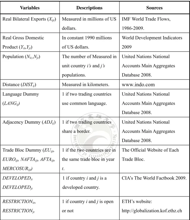
(41) Table 9. Variables and data sources. Variables. Descriptions. Sources. Real Bilateral Exports (Xijt). Measured in millions of US. IMF World Trade Flows,. dollars.. 1986-2009.. Real Gross Domestic. In constant 1990 millions. World Development Indicators. Product (Yit,Yjt). of US dollars.. 2009. Population (Nit,,Njt). The number of Measured in. United Nations National. unit country i’s and j’s. Accounts Main Aggregates. populations.. Database 2008.. Distance (DISTij). Measured in kilometers.. www.indo.com. Language Dummy. 1 if two trading countries. United Nations National. (LANGij). use common language.. Accounts Main Aggregates Database 2008.. Adjacency Dummy (ADJij). 1 if two trading countries. United Nations National. share a border.. Accounts Main Aggregates Database 2008.. Trade Bloc Dummy (EUijt,. 1 if the two countries are in. The Official Website of Each. EUROijt, NAFTAijt, AFTAijt,. the same trade bloc in year. Trade Bloc.. MERCOSURijt). t.. DEVELOPEDit. 1 if country i and j is a. DEVELOPEDjt. developed country.. RESTRICTIONit,. 1 if country i and j is open. ETH’s website:. RESTRICTIONjt. or not. http://globalization.kof.ethz.ch. 35 . CIA’s The World Factbook 2009..

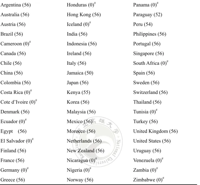
(42) Table 10. List of 41 exporting and 57 importing countries. Argentina (56). Honduras (0)#. Panama (0)#. Australia (56). Hong Kong (56). Paraguay (52). Austria (56). Iceland (0)#. Peru (54). Brazil (56). India (56). Philippines (56). Cameroon (0)#. Indonesia (56). Portugal (56). Canada (56). Ireland (56). Singapore (56). Chile (56). Italy (56). South Africa (0)#. China (56). Jamaica (50). Spain (56). Colombia (56). Japan (56). Sweden (56). Costa Rica (0)#. Kenya (55). Switzerland (56). Cote d’Ivoire (0)#. Korea (56). Thailand (56). Denmark (56). Malaysia (56). Tunisia (0)#. Ecuador (0)#. Mexico (56). Turkey (56). Egypt. Morocco (56). United Kingdom (56). El Salvador (0)#. Netherlands (56). United States (56). Finland (56). New Zealand (56). Uruguay (56). France (56). Nicaragua (0)#. Venezuela (0)#. Germany (0)#. Nigeria (0)#. Zambia (0)#. Greece (56). Norway (56). Zimbabwe (0)#. (56). Note: The data set of 2282 trading country pairs includes 41 exporting and 57 importing countries over the period 1986-2008. For each country, the number in the bracket denotes the number of its export destinations in the data set. # denotes a country that is a trade destination but not trade origin country in the data set.. 36 .

(43) Table 11. Trade blocs and selected member countries. Trade bloc. Year enforced. Member countries Belgium (1950), France (1950)*, Germany (1950)*, Italy (1950)*, Luxembourg (1950) , The Netherlands (1950), Denmark (1973)*, Ireland (1973)*, The United Kingdom (1973)*, Greece (1981)*, Spain (1986)*,. EU (27). 1957. Portugal (1986)*, Austria (1995)*, Finland (1995)*, Sweden (1995)*, Czech Republic (2004), Cyprus (2004), Estonia (2004), Latvia (2004), Lithuania (2004), Hungary (2004), Malta (2004), Poland (2004), Slovenia (2004), Slovakia (2004), Bulgaria (2007), Romania (2007). Austria (1999)*, Belgium (1999), Finland (1999) *, France (1999)*, Germany (1999)*, Ireland (1999)*,. EURO (16). 1999. Italy (1999)*, Luxembourg (1999), Netherlands (1999)*, Portugal (1999)*, Spain (1999)*, Greece (2001)*, Slovenia (2007), Cyprus (2008), Malta (2008), Slovakia (2009).. NAFTA (3). 1989. Canada (1989)*, USA (1989)*, and Mexico (1994)*. Brunei Darussalam (2002), Cambodia (2002), Indonesia. AFTA (10). 2002. (2002)*, Laos (2002), Malaysia (2002)*, Myanmar (2002), Philippines (2002)*, Singapore (2002)*, Thailand (2002)*, Viet Nam (2002).. MERCOSUR (5). 1994. Argentina (1994)*, Brazil (1994)*, Paraguay (1994)*, Uruguay (1994)*, Venezuela (2006)*.. Note: Total number of member countries of each trade bloc is shown in a parenthesis in column one. In column three the member in a parenthesis is the year when a member country enters into the trade bloc. * denotes a country that is selected member in the data set.. 37 .

(44) Table 12. List of developed and developing countries and country dummies. Developed. Developing. Exporter. Importer. countries. countries. dummy. dummy. ◎. exporter01. importer01. Argentina Australia. ◎. exporter02. importer02. Austria. ◎. exporter03. importer03. exporter04. importer04. exporter05. importer05. Brazil Canada. ◎ ◎. Chile. ◎. exporter06. importer06. China. ◎. exporter07. importer07. Colombia. ◎. exporter08. importer08. exporter09. importer09. exporter10. importer10. Denmark. ◎. Egypt. ◎. Finland. ◎. exporter11. importer11. France. ◎. exporter12. importer12. Greece. ◎. exporter13. importer13. Hong Kong. ◎. exporter14. importer14. India. ◎. exporter15. importer15. Indonesia. ◎. exporter16. importer16. Ireland. ◎. exporter17. importer17. Italy. ◎. exporter18. importer18. exporter19. importer19. exporter20. importer20. exporter21. importer21. exporter22. importer22. Jamaica Japan. ◎ ◎. Kenya Korea. ◎ ◎. Malaysia. ◎. exporter23. importer23. Mexico. ◎. exporter24. importer24. Morocco. ◎. exporter25. importer25. Netherlands. ◎. exporter26. importer26. New Zealand. ◎. exporter27. importer27. Norway. ◎. exporter28. importer28. Paraguay. ◎. exporter29. importer29. Peru. ◎. exporter30. importer30. Philippines. ◎. exporter31. importer31. exporter32. importer32. Portugal. ◎. 38 .

(45) Singapore. ◎. exporter33. importer33. Spain. ◎. exporter34. importer34. Sweden. ◎. exporter35. importer35. Switzerland. ◎. exporter36. importer36. Thailand. ◎. exporter37. importer37. Turkey. ◎. exporter38. importer38. exporter39. importer39. exporter40. importer40. exporter41. importer41. United Kingdom (UK). ◎. Uruguay United States (USA). ◎ ◎. Cameroon. ◎. importer42. Costa Rica. ◎. importer43. Cote d’Ivoire. ◎. importer44. Egypt. ◎. importer45. El Salvador. ◎. importer46. Germany. importer47. ◎. Honduras Iceland. ◎. importer48 importer49. ◎. Nicaragua. ◎. importer50. Nigeria. ◎. importer51. Panama. ◎. importer52. South Africa. ◎. importer53. Tunisia. ◎. importer54. Venezuela. ◎. importer55. Zambia. ◎. importer56. Zimbabwe. ◎. importer57. Note: 1. According to the CIA’s The World Factbook 2009, a country is defined as a developed country (a high-income economy) if it’s gross national income (GNI) in year 2005 was higher and equal to $10,726, otherwise denoted as a developing country. 2. According to the World Bank Atlas method, a country is defined as a developed country (a high-income economy) if it’s gross national income (GNI) in year 2009 was higher and equal to $12,196, otherwise denoted as a developing country.. 39 .

(46) Table 13. Main regression results for various models. Model. PCS. lnY_it. 1.166 (0.015) **. lnY_jt. 0.795 (0.015) **. lnN_it. FE3-2. FE2. 1.316 (0.062) **. 1.386 (0.071) **. 1.290 (0.046) **. 1.290 (0.046) **. 1.278 (0.063) **. 1.308 (0.073) **. 1.248 (0.047) **. 1.248 (0.047) **. -0.066 (0.016) **. 0.090 (0.069). 0.047 (0.079). 0.159 (0.051) **. 0.159 (0.051) **. lnN_jt. 0.104 (0.015) **. 0.090 (0.158). 0.294 (0.180). 0.354 (0.118) **. 0.354 (0.118) **. lnDist_ij. -0.886 (0.014) **. -1.300 (0.013) **. LANG_ij. 0.748 (0.025) **. 0.765 (0.024) **. ADJ_ij. 0.287 (0.058) **. -0.280 (0.049) **. RESTRICTIONS_it. 0.017 (0.001) **. 0.019 (0.001) **. 0.016 (0.002) **. 0.020 (0.001) **. 0.020 (0.001) **. RESTRICTIONS_jt. 0.020 (0.001) **. 0.012 (0.001) **. 0.011 (0.001) **. 0.012 (0.001) **. 0.012 (0.001) **. SIMILAR_ijt. 0.625 (0.108) **. -2.800 (0.112) **. -1.520 (0.128) **. -4.277 (0.496) **. -4.277 (0.496) **. IIT_ijt. 1.573 (0.033) **. 1.088 (0.028) **. 1.841 (0.031) **. 0.839 (0.027) **. 0.839 (0.027) **. BOTHDEVELOPED_ijt. -0.376 (0.037) **. -2.850 (0.253) **. -2.308 (0.289) **. (drop). -1.457 (0.853) **. BOTHDEVELOPING_ijt. 0.163 (0.035) **. 2.403 (0.252) **. 2.549 (0.289) **. (drop). 1.907 (0.792) **. EU_ijt. -0.608 (0.053) **. -0.430 (0.047) **. 1.001 (0.051) **. 0.116 (0.084). EURO_ijt. FE3-1. -0.015 (0.067). -0.015 (0.067). 0.128 (0.071). 0.180 (0.081). 0.061 (0.059). 0.061 (0.059). 0.807 (0.166) **. 2.235 (0.186) **. 0.688 (0.223) **. 0.688 (0.223) **. NAFTA_ijt. -0.132 (0.198) **. AFTA_ijt. 2.171 (0.174) **. 0.066 (0.145). 2.259 (0.165) **. MERCOSUR_ijt. 2.018 (0.149) **. 1.967 (0.125) **. 4.285 (0.138) **. Constant. -1.587 (0.262) **. -9.170 (3.141) **. -25.498 (3.588) **. -0.278 (0.122) 0.416 (0.137) ** -22.503 (2.211). -0.278 (0.122) 0.416 (0.137) ** -30.173 (2.254) **. Observations. 52486. 52486. 52486. 52486. 52486. Parameters. 40. 135. 132. 2316. 2316. Sum of squares. 170494.402. 112546.673. 147393.020. 58178.010. 58178.010. Adjusted R. 0.711. 0.809. 0.749. 0.896. 0.896. AIC. 4.097. 3.685. 3.955. 3.119. 3.119. BIC. -324268.220. -343377.407. -330326.837. -351829.405. -350793.625. 2. Note: Standard errors in parentheses. **Significant at the 5 percent level.. 40 . FEG.

(47) Table 14. Estimated exporter and importer dummies and country-pair dummies. exporter. importer. REI. Indonesia. Malaysia. Malaysia. Philippines. Singapore. Thailand. Austria. Denmark. αi. αj. αi+αj. AFTA. -0.0017. 1.8439. 1.8421. 4.0620. yes. Philippines. AFTA. -0.0017. 1.4508. 1.4491. 3.7742. yes. Singapore. AFTA. -0.0017. 5.0471. 5.0454. 8.3016. yes. Thailand. AFTA. -0.0017. 1.3682. 1.3665. 3.0084. yes. Indonesia. AFTA. 1.8197. 0.2696. 2.0893. 3.5881. yes. Philippines. AFTA. 1.8197. 1.4508. 3.2705. 5.5933. yes. Singapore. AFTA. 1.8197. 5.0471. 6.8668. 10.8646. yes. Thailand. AFTA. 1.8197. 1.3682. 3.1880. 5.5325. yes. Indonesia. AFTA. 0.1856. 0.2696. 0.4552. 2.2983. yes. Malaysia. AFTA. 0.1856. 1.8439. 2.0295. 5.4699. yes. Singapore. AFTA. 0.1856. 5.0471. 5.2327. 8.8565. yes. Thailand. AFTA. 0.1856. 1.3682. 1.5539. 4.4698. yes. Indonesia. AFTA. 4.3917. 0.2696. 4.6613. 7.0166. yes. Malaysia. AFTA. 4.3917. 1.8439. 6.2356. 10.4357. yes. Philippines. AFTA. 4.3917. 1.4508. 5.8425. 8.5569. yes. Thailand. AFTA. 4.3917. 1.3682. 5.7599. 8.4708. yes. Indonesia. AFTA. 1.1934. 0.2696. 1.4630. 2.9246. yes. Malaysia. AFTA. 1.1934. 1.8439. 3.0372. 5.5607. yes. Philippines. AFTA. 1.1934. 1.4508. 2.6442. 4.3166. yes. Singapore. AFTA. 1.1934. 5.0471. 6.2405. 9.2432. yes. Denmark. EU. 1.7996. 2.7606. 4.5601. 4.4382. no. Finland. EU. 1.7996. 2.6737. 4.4732. 4.2785. no. France. EU. 1.7996. 1.6579. 3.4574. 2.0069. no. Greece. EU. 1.7996. 3.1177. 4.9173. 4.3884. no. Ireland. EU. 1.7996. 3.0636. 4.8632. 4.3402. no. Italy. EU. 1.7996. 1.7804. 3.5800. 3.0026. no. Netherlands. EU. 1.7996. 3.8485. 5.6481. 4.1389. no. Spain. EU. 1.7996. 2.2353. 4.0348. 2.9806. no. Sweden. EU. 1.7996. 2.5893. 4.3889. 4.0458. no. UK. EU. 1.7996. 2.1683. 3.9679. 2.2852. no. Germany. EU. 1.7996. 1.6910. 3.4906. 3.5193. yes. Portugal. EU. 1.7996. 3.3837. 5.1832. 4.2377. no. Austria. EU. 2.0962. 1.9781. 4.0743. 4.0164. no. Finland. EU. 2.0962. 2.6737. 4.7699. 5.5163. yes. France. EU. 2.0962. 1.6579. 3.7541. 1.8936. no. 41 . αij. αij is higher.