Modified Relay Feedback Approach for Controller Tuning Based on Assessment of Gain and Phase Margins

Subscriber access provided by NATIONAL TAIWAN UNIV

Industrial & Engineering Chemistry Research is published by the American Chemical Society. 1155 Sixteenth Street N.W., Washington, DC 20036

Article

Modified Relay Feedback Approach for Controller Tuning

Based on Assessment of Gain and Phase Margins

Jyh-Cheng Jeng, Hsiao-Ping Huang, and Feng-Yi Lin

Downloaded from http://pubs.acs.org on November 18, 2008

More About This Article

Additional resources and features associated with this article are available within the HTML version: • Supporting Information

• Access to high resolution figures

• Links to articles and content related to this article

Modified Relay Feedback Approach for Controller Tuning Based on Assessment

of Gain and Phase Margins

Jyh-Cheng Jeng, Hsiao-Ping Huang,* and Feng-Yi Lin

Department of Chemical Engineering, National Taiwan UniVersity, Taipei 106, Taiwan

A relay feedback based method for tuning a PI/PID (proportional-integral-derivative) controller with an assessment of gain and phase margins is proposed. The proposed method estimates the gain and phase margins of an existing control system by a modified relay feedback scheme, where a delay element is embedded between the relay and controller. The gain and phase margins of a control system are used to assess the control performance. When the controller is found not in good performance, the proposed method is then applied to retune the PI/PID controller based on gain- and phase-margin specifications. Simulation results have shown that the proposed method is effective for processes with different kinds of dynamics and for multiloop systems.

1. Introduction

The proportional-integral-derivative (PID) controller is widely used in chemical process industries because of its simple structure and robustness to modeling error. Despite the fact that numerous PI/PID tuning methods have been provided in the literature, many control loops are still found to perform poorly.1

Therefore, regular performance assessment and controller tuning are necessary. In process control, minimum variance has been used as a benchmark for assessing the closed-loop performance for decades.2_{The other approach to assess the performance is}

based on the system’s dynamic characteristics. Along this second approach, gain and phase margins have been served as important measures of performance and robustness in single-input-single-output (SISO) systems. It is known from classical control theory that the phase margin is related to the damping of the system and that the error-based performance indices are related to these stability margins.3_{For the multiloop control of a}

multiinput-multioutput (MIMO) system, gain and phase margins can also be defined in the similar spirit as for a SISO system based on the effective open-loop process (EOP).4_{Traditionally, under the}

assumption that the process model and controller parameters are known, the gain and phase margins are obtained by solving nonlinear equations numerically or by graphical, trial-and-error use of Bode’ plots. Because calculation of gain and phase margins in such ways is very tedious, Ho and co-workers5,6

derived approximate analytical formulas to compute gain and phase margins of PI/PID control systems using a first-order plus dead-time (FOPDT) process model. However, the assumption is not practical because the process model and controller settings may be unknown at the stage of performing the performance assessment. Thus, it is desirable to find a procedure for estimation of gain and phase margins. Recently, Ma and Zhu7

proposed a performance assessment procedure for a SISO system based on modified relay feedback. Gain and phase margins are estimated by two relay tests, where an ideal relay is used for the first test and a relay with hysteresis is used for the other. Because of a linear assumption about the amplitude of the limit cycle, their method may not give accurate results for processes with more complex dynamics such as a process with right-half-plane (RHP) zero and oscillatory modes.

Controller designs to satisfy gain- and phase-margin speci-fications are well-accepted in practice for classical control. To

be free of the tedious modeling and computation procedures aforementioned, Åstro¨m and Ha¨gglund8_{used relay feedback for}

automatic tuning of PID controllers with specification on either gain margin or phase margin, but it cannot achieve both specifications simultaneously. Some approximate analytical PI/ PID tuning formulas have been derived to achieve the specified gain and phase margins.9,10_{Most of them use simplified models}

such as the FOPDT model or the second-order plus dead-time (SOPDT) model. For processes with more complicated dynam-ics, the resulting control systems may not be able to achieve user-specified gain and phase margins exactly. Ho et al.11

extended the earlier work of Ho et al.9_{for tuning of multiloop}

PID controllers based on gain- and phase-margin specifications. In this paper, a method for controller tuning with assessment of gain and phase margins based on a modified relay feedback test is proposed. This modified relay feedback embeds an additional delay between the relay and controller. The gain and phase margins are used to assess the performance and robustness of the control systems which have unknown controller param-eters and process dynamics. For multiloop systems, the modified relay tests are conducted in a sequential manner to estimate the gain and phase margins of each loop. The estimated results can be used to indicate the appropriateness of the controller param-eters. When the retuning of a controller is found necessary, a similar procedure can be applied to tune the PI/PID controller based on the user-specified gain and phase margins, where pro-cess models are not required. In this way, performance assessment and controller retuning can be done with the same approach, which ensures a good performance of the control system.

This paper is organized as follows. Section 2 describes the proposed modified relay feedback structure. Procedures for performance assessment and controller design are presented in Sections 3 and 4, respectively. Section 5 extends the methods to multiloop control systems. Simulation examples follow in Section 6 to demonstrate the procedures and effectiveness of the proposed methods. Conclusions are drawn in Section 7.

2. Modified Relay Feedback Structure

The use of relay feedback for automatic tuning of PID controllers was first proposed by Åstro¨m and Ha¨gglund.8_The

block diagram of the standard relay feedback system is as shown in Figure 1a. The system generates a continuos cycling if it has a phase lag of at leastπ. A limit cycle with a period Puresults,

and this period is the ultimate period. Therefore, the ultimate

* Corresponding author. Tel.: 886-2-2363-8999. Fax: 886-2-2362-3935. E-mail: [email protected].

10.1021/ie051310z CCC: $33.50 © 2006 American Chemical Society Published on Web 05/02/2006

frequency from this relay feedback test is

From the describing function approximation, the ultimate gain can be approximately given by

where h is the relay output magnitude and a is the amplitude of the limit cycle. In other words, one point, i.e., the critical point, on the Nyquist curve of the process can be obtained from the relay feedback test.

For the purpose of performance assessment, a modified relay feedback structure is proposed as shown in Figure 1b, where Gc, G, ur, and y are the controller, process, relay output, and

process output, respectively. Moreover, a delay element, e-∆s, is embedded between the relay and the controller. Notice that the insertion of additional delay was also studied in some conventional relay feedback systems to estimate process fre-quency responses at different frequencies.12-14 _{But, in these}

studies, the PID controller was disconnected and isolated from the relay feedback loop. Compared with the conventional relay feedback, the most important features of this modified structure are that the controller is always in line with the process with an additional delay being embedded. Because of the first feature, the gain and phase margins can be obtained. In contrast, the conventional relay feedback gives only the ultimate gain and ultimate period regarding the open-loop process. Besides, the inserted additional delay is used to obtain other points (other than the critical point) on the Nyquist curve, which are helpful for the estimation of phase margin. Even though other points on the Nyquist curve can also be obtained by inserting other elements or by relay with hysteresis,7,8,15_{this proposed structure}

can ensure the existence of a limit cycle even for a low-order process without time delay. As a result, it can assess the performance of an existing closed-loop system by estimation of its gain and phase margins, as presented in the following section, to determine if a retuning of the controller is necessary.

3. Performance Assessment

As has been mentioned, gain and phase margins are good measures for the performance and robustness of control systems. However, without any information about the controller and process, it is impossible to calculate the gain and phase margins by solving equations analytically, numerically, or graphically.

In this section, a systematic procedure that can estimate gain and phase margins of a completely unknown system by the proposed modified relay feedback test is presented to assess the performance of the control system.

3.1. Estimation of Gain Margin. Consider the modified relay

feedback system as shown in Figure 1b. For the estimation of gain margin, by setting∆ as zero, the frequency known as phase crossover frequency,ωp, which has a phase lagπ, is required.

Let the loop transfer function be GLP(s) ) Gc(s)G(s). The system

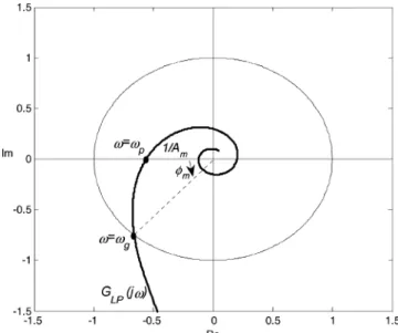
starts to oscillate and then attain a limit cycle. The oscillating point is the intersection of the Nyquist curve of GLP(s) and the

negative real axis in the complex plane, as shown in Figure 2. The phase crossover frequency of GLP(s) can be calculated by

eq 1 asωp) 2π/Pp, where Ppis the period of the limit cycle.

In addition, using the approximation of describing function, the amplitude of GLP(s) can be calculated by eq 2 as|GLP(jωp)| ) πa/4h. However, the accuracy of such an approximation is poor in some cases where the error may be as large as 20%.16_For

more accurate estimation,|GLP(jωp)| can be computed based

on Fourier analysis as17,18

Therefore, the gain margin, Am, can be estimated as

3.2. Estimation of Phase Margin. When the estimation of

gain margin is finished, the delay ∆ is then set as a nonzero value in order to extract the frequency information of GLP(s) at

some frequency other than ωp for the estimation of phase

margin. With a given value of ∆, assume that the system oscillates with a period of P, and then we have the phase of the system as

whereω ) 2π/P. To calculate the phase margin, the desired frequency is the gain crossover frequency,ωg, of GLP(s), which

is the intersection of the Nyquist curve of GLP(s) and the unit

circle in the complex plane, as shown in Figure 2. The desired value of∆ that makes the amplitude of GLP(jωg) equal unity is

denoted ∆d, and the period of the limit cycle is Pg. In other Figure 1. (a) Standard relay feedback system; (b) modified relay feedback

system.

ω_u) 2π

P_u (1)

K_u) 4h

πa (2)

Figure 2. Estimation of gain and phase margins.

|GLP(jωp)| ) |

∫

∫

words, the gain crossover frequency of GLP(s) equals the phase

crossover frequency of GLP(s) e-∆s. In this case, eq 5 can be

written as arg{GLP(jωg)}- ∆dωg) -π, where ωg) 2π/Pg.

Then, it follows that the phase margin, φm, can be estimated as

To find the value of ∆d, an iterative method such as that

proposed by Chen et al.14 _{can be used. Here, an iterative}

procedure such as the following is presented. Starting from an initial guess∆(0)_{, the value of∆ is updated by}

where γ(i) _{> 0 is the convergence rate and |G}

LP(jω(i))| is

computed by

Notice that we have ∆d ) 0 if Am ) 1 and, in general, ∆d

increases as Am and Pp increase. Thus, the value of ∆(0) is

suggested as (Am- 1)Pp/6. In addition,γ(i)is chosen as

which makes eq 7 have a quadratic convergence rate near the solution.8_{In each iteration, the value of∆}(i)_{holds constant until}

the output generates two or three oscillating cycles and then switches to the next value in an on-line adaptive way. When eq 7 converges, the resulting value of∆ is taken as ∆d.

3.3. Assessment of Performance. With the estimated gain

and phase margins, the robustness of the current system can be assessed. The recommended ranges of gain and phase margins are between 2 and 5 and between 30° and 60°, respectively. Nevertheless, gain and phase margins indeed are closely related to the time-domain performance of the system.

For set-point tracking, a control system with gain margin 2.1 and phase margin 60° can have the optimal integral of the absolute value of the error (IAE).19 _{The corresponding loop}

transfer function is as the following form,

whereθ is the apparent dead-time of the process. For inverse-based controller design, such as internal model control (IMC) design, the loop transfer function has the following form,

where k is a user-specified parameter to make a tradeoff between the speed of the response and the robustness of the closed-loop system. The gain and phase margins of the resulting closed-loop system satisfy the following relation:

In general, the above-mentioned inverse-based design can give a system a good set-point response and has an optimal IAE value if the value of k is chosen as k ) 0.59/θ,19_which

corres-ponds to Am) 2.6 and φm) 55°. Thus, if eq 12 is not satisfied

by the estimated gain and phase margins, the set-point perfor-mance is not satisfactory. On the other hand, this inverse-based controller also gives marginally acceptable disturbance response in the case of dead-time-dominant processes, but results in a sluggish disturbance response when process lag is dominant.20

In the case of a lag-dominant process, if good disturbance re-sponse is desirable, the gain and phase margin pair (Am, φm)

has to follow the curve as shown in Figure 3. In fact, this curve is obtained from a control system where the controller is synthe-sized to achieve optimal IAE value under constant Msin

re-sponse to a step disturbance.21_{Each point on that curve}

corres-ponds to a given value of Ms which is the maximum of the

magnitude of the sensitivity function, 1/(1 + GcG(jω)). In

general, dynamics of chemical plants can be represented by an FOPDT model which is characterized by apparent dead time, θ, and apparent time constant, τ. On the basis of this FOPDT dynamics, the controller for disturbance rejection under a con-stant Mscan be synthesized by assigning an optimal sensitivity

function.21_{For dead-time-dominant processes (i.e., smallτ/θ),}

the gain and phase margins of such a synthesized system vary withτ/θ. Nevertheless, for a lag-dominant process where the τ/θ is large, the resulting gain and phase margins approach to some constant values. The pairs of such constant gain and phase margins at different Msvalues give the result as shown in Figure

3. The value of Ms can be used to make a tradeoff between

control performance and system robustness. If the estimated (Am, φm) pair is far away from the curve, the disturbance performance

may be poor. Therefore, based on the gain and phase margins, not only the system robustness but also the possibility of achieving good control performance can be assessed.

4. Controller Tuning

After assessment, when the performance of the control system is found to be poor, the controller needs to be retuned. The modified relay feedback scheme can be applied for on-line tuning of a PI/PID controller to achieve user-specified gain and phase margins, designated as A*_mand φ*_m, respectively. By this way, neither an intermediate process model nor nonlinear equation solving is required.

4.1. Tuning of PI Controller. Consider the PI controller of

the following transfer function. φ_m) arg{G_LP(jωg)}+ π ) ∆dωg (6)

∆(i+1)) ∆(i)- γ(i)(|G_LP(jω(i))| - 1) (7)

|GLP(jω (i)

)| )|G_LP(jω(i)) e-jω(i)∆(i)| ) |

∫

∫

(

)

Figure 3. Gain and phase margins for good disturbance performance.

G_c(s) ) k_c

(

)

For a given value of∆, the parameters, kcandτI, can be found

to satisfy the specification of phase margin. In other words, they can be found such that the following two equations hold.

By the modified relay feedback test, eq 14 can be satisfied by adjusting the value ofτIand eq 15 can be satisfied by adjusting

the value of kc. However, the specification of gain margin may

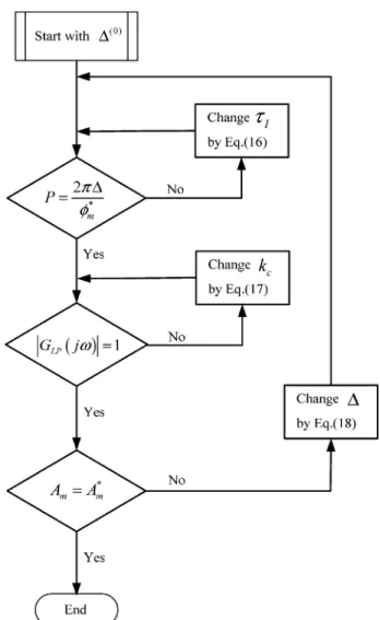
not be necessarily achieved by such obtained controller param-eters. In general, the gain margin of the resulting system aforementioned, i.e., the system with φm) φ*m, is a function of ∆ value. Therefore, there exists a certain value of ∆ which can make the gain margin of the resulting system meet its specifica-tion. According to the analysis, an iterative procedure for tuning the PI controller using the modified relay feedback test is presented as follows:

(1) Start with a guessed value of∆, i.e., ∆(0) .

(2) AdjustτIby the following equation:

where P(i)_{is the period of the limit cycle in the ith iteration.}

Equation 14 holds when eq 16 converges.

(3) Adjust kcby the following equation until it converges so

that eq 15 holds,

whereω(i)_{) 2π/P}(i)_and|G

LP(jω(i))| is computed by eq 8.

(4) Set∆ ) 0, and estimate Amby eq 4.

(5) Check if the estimated Amequals A*m. If not, change the

value of ∆ by the following equation and go back to step 2 until Am) A*mholds.

The convergence rates,γ₁(i),γ₂(i), andγ₃(i), can be defined in the similar manner of eq 9 as

Notice thatγ₁(i)< 0, γ₂(i)> 0, and γ₃(i)> 0. For an FOPDT pro-cess, inserting a delay∆ in the relay feedback loop approximately results in an increase of 4∆ in the period of the limit cycle. To improve the convergence of eq 16, it is desirable that 2π∆/φ*_m ) P ≈ (Pp+ 4∆). Thus, the initial guess of ∆ is suggested as

This design procedure is shown graphically in Figure 4.

The procedure is performed in an on-line adaptive manner. In each of the iterations, two or three oscillating cycles are generated from the modified relay feedback test to compute the required quantities for the next iteration. When the value of∆ converges, the resulting controller parameters are the desired ones which can make the control system have both user-specified gain and phase margins.

4.2. Tuning of PID Controller. For the tuning of a PID

controller, a similar procedure can be applied. The PID controller transfer function is given as

Since there is one more parameter to be tuned, an additional condition must be introduced to determine the parameters uniquely. The derivative time,τD, is usually chosen as a fixed

ratio of the integral time,τI, as

Researchers8,22 _{have recommended that R ) 0.25. With the}

relation of eq 24, the procedure for PI controller tuning presented in the previous section can be applied directly to tune the PID controller.

IfτDis not chosen as a fixed ratio toτI, then the extra degree

of freedom can be used to achieve another performance require-ment. For example, Chen et al.14_{introduced the “flat-phase}

con-dition” to determine the value of R. By making the phase deriv-φ*_m) ∆ω_g or P_g) 2π∆ φ*_m (14) |GLP(jωg)|)|GLP(jωg) e -jωg∆|) |

∫

∫

τ_I(i+1)) τ_I(i)- γ₁(i)

(

φ*_m

)

k_c(i+1)) k_c(i)- γ₂(i)(|G_LP(jω(i))| - 1) (17)

∆(i+1)) ∆(i)- γ₃(i)(A_m(i)- A*_m) (18)

γ1 (i)₎ τI (i)_{- τ} I (i-1) P(i)- P(i-1) (19) γ₂(i)) kc (i)_{- k} c (i-1) |GLP(jω (i)_{)| - |G} LP(jω (i-1)_)| (20) γ3

(i)_{) ∆}(i)- ∆(i-1) A_m(i)- A_m(i-1) (21) ∆(0)) Pp 2π φ*_m- 4 (22)

Figure 4. Design procedure of PI controller.

G_c(s) ) k_c

(

+ τ_Ds

)

τ_D) Rτ_I (24)

ative with respect to the frequency being zero at a given frequency called the “tangent frequency”, a relationship between τI and τD for the robust PID controller can be obtained.

Moreover, Zhuang and Atherton23 _{discuss the tuning of PID}

controller to achieve an optimal integral time-weighted square error (ITSE) performance criterion and suggest the value of R as

where κ is the process-normalized gain defined by κ )|G(j0)/ G(jωu)|. To use eq 25, the steady-state gain and ultimate gain

of the process are required. This information can be estimated from the modified relay feedback test by setting∆ ) 0, kc) 1, τD) 0, and τIas a very large value. In fact, such setting restores

the modified relay feedback to the conventional relay feedback scheme. Of course, this is at the cost of an extra experiment.

4.3. Specification of Gain and Phase Margins. There are

some restrictions on the specification of the gain and phase margin pairs. One usual requirement is that the controller param-eters have to be positive. Ho et al.9_{have provided the feasible}

region of gain- and phase-margin specifications for PI and PID control based on FOPDT and SOPDT process models, respec-tively. But the region depends on the parameters of the model. Generally speaking, if a larger gain margin is specified, a higher value of phase margin should also be specified accordingly.

To achieve better performance, the specification of (Am, φm)

pair has to consider the control objective. As has been mentioned in Section 3.3, for set-point tracking, it is suitable to specify (Am, φm) pair by eq 12. For disturbance rejection, eq 12 can also be

used for dead-time-dominant processes. On the other hand, Fig-ure 3 can be used to specify (Am, φm) for lag-dominant processes. 5. Extension to Multiloop Systems

Multiloop SISO controllers are often used to control chemical plants which have MIMO dynamics. Ho et al.11_{defined the gain}

and phase margins based on the Gershgorin bands of the multiloop system. However, according to their definition, the gain and phase margins of each loop are independent of the controllers in the other loops, so that the interactions between loops are not considered. In this paper, the gain and phase margins are defined in the similar spirit as for a SISO system, based on the effective open-loop process (EOP) in the work of Huang et al.4_{The ith EOP describes the effective transmission}

from the ith input to the ith output when all other loops are closed. With the formulation of EOP, the multiloop control system can be considered as several equivalent SISO loops.

Consider the multiloop control system of a 2× 2 multivari-able process with the following process and controller transfer function matrices, G(s) and GC(s).

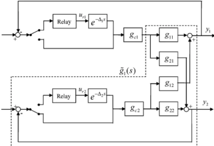
The mathematical definitions of the two EOPs, g˜1(s) and g˜2(s),

are given as4

where

On the basis of the EOPs of eq 28, the loop transfer functions of the equivalent loops are GLP,1(s) ) gc1(s)g˜1(s) and GLP,2(s) ) gc2(s)g˜2(s). Therefore, as in the case of SISO system, the

gain and phase margins of each loop can be estimated by sequentially using the proposed modified relay feedback system. Figure 5 shows the modified relay feedback scheme for the first loop, where loop 1 is under relay mode and loop 2 is under control mode. In a similar way, the gain and phase margins of the second loop can be estimated. This procedure can be extended to a general multiloop system, where the modified relay tests are conducted in a sequential manner to estimate the gain and phase margins of each loop. Since the mathematical formulation of EOPs for high-dimensional processes is complex, calculation of gain and phase margins from process models in the traditional way becomes very difficult. However, the proposed procedure can be easily applied in high-dimensional processes regardless of the complexity of the EOPs.

When retuning of the controller is found necessary, a similar procedure like the case of a SISO system can be applied to tune the controller gci(s) to meet the specification of gain and

phase margins of the ith loop. If gain and phase margins of more than one loop are simultaneously specified, the controller tuning needs to go through an iterative procedure because of the interaction nature of a multiloop system. In that case, gain and phase margins should be carefully specified to ensure the convergence of the controller parameters.

6. Simulation Examples

It is inevitable that measured output will be contaminated by some noise. To reduce the effect of noise, cycling data used in the estimation procedure can be taken as the ensemble average of constant cycles. However, this takes more experiments and more cost. To avoid this, it is suggested that the measured out-puts are first pretreated by a filter before being used for the com-putation. During the relay feedback experiment, the input and output are periodical signals. The wavelet transform24_{is the one}

most efficient for filtering such periodical signals. The original signal is decomposed into different frequency contents through wavelet transform, and then high frequency parts, which are usually the measurement noise, are dropped to form the filtered signal. The wavelet-filtering techniques are well-developed and can be found in existing computer software (e.g., Matlab). After

R ) 0.413 3.302κ + 1 (25) G(s) )

[

]

[

]

Figure 5. Modified relay feedback scheme for a 2× 2 multiloop system.

h_i(s) ) gci(s)gii(s)

the measurements are denoised, the proposed procedures are then applied, and, hence, accurate results can be obtained. The wave-lets used in following simulation work are the discrete Meyer wavelets.

Example 1. Consider a control system with an FOPDT

process and a PI controller given by

Three different values of the dead time,θ ) 0.5, 1, and 1.5, are used for the simulation. As shown in Table 1, the actual gain and phase margins, designated as Ahmand φhm, for these

three cases cover a wide range. On the basis of the proposed relay feedback test, the estimated gain and phase margins together with the values of∆(i)_{during iteration are shown in}

Table 1 for comparison. The value of∆ converges after two iterations. It can be seen from Table 1 that the estimated gain and phase margins are very close to the actual ones.

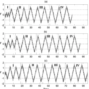
Then, simulation is conducted under noisy condition where white noise with 15% noise-to-signal ratio (NSR) is introduced. Here, the NSR is defined by

The wavelet filtering is performed on the output on each iteration. Then, data are computed for the next iteration. The output responses during the estimation procedure are shown in Figure 6, where period I is for estimating gain margin and per-iods II-IV are for estimating phase margin; the filtered outputs are shown in Figure 7. The estimated results are also given in

Table 1. It can be seen that, by filtering the output, good estima-tion accuracy can be obtained without extensive experiments. For the case ofθ ) 1.5, because the gain and phase margins of the control system (1.31 and 18.2°) are quite away from the recommended ranges, the performance and robustness are poor. Thus, retuning of the controller is needed. We specify the gain margin as A*_m ) 2.5, and then the phase margin is specified according to eq 12 as φ*_m) 54°. This design is equivalent to the IMC design, so that the control system is expected to have good set-point response. The tuning procedure is shown in Table 2. The results converge after two iterations of∆ (∆(2)) 2.239),

and the PI controller is obtained as

The actual gain and phase margins of this resulting control system are Am) 2.49 and φm) 53.2°, which are very close to

the specified ones. When measurement noise is introduced, the output is filtered and a similar PI controller with kc ) 0.434

andτI ) 1.01 results. The closed-loop responses before and

after retuning are shown in Figure 8, where the performance is significantly improved after controller retuning.

Example 2. Consider a second-order process and a PID

controller given by

The actual gain and phase margins are 2.63 and 56.5°, respec-tively. On the basis of the modified relay feedback, the estimated gain and phase margins are Am) 2.62 and φm) 56.1°, where the

value of∆ converges after two iterations with ∆(0)_{) 1.089, ∆}(1) ) 1.298, and ∆(2)) 1.655. According to the estimated result,

this control system is expected to have good set-point response

Table 1. Actual and Estimated Gain Margin and Phase Margin in Example 1 actual estimated (without noise) estimated (with noise) θ Ahm φhm Am φm ∆(0) ∆(1) ∆(2) (∆d) Am φm 0.5 4.64 61.5° 4.56 60.7° 1.278 1.359 1.423 4.47 60.0° 1 2.11 40.0° 2.07 39.4° 0.789 0.864 0.924 2.15 39.1° 1.5 1.33 18.6° 1.31 18.2° 0.336 0.385 0.427 1.41 18.1° G(s) ) e -θs s + 1, Gc(s) ) 0.616

(

)

Figure 6. Output response with noise during performance assessment in

example 1: (a)θ ) 0.5, (b) θ ) 1, and (c) θ ) 1.5.

Figure 7. Filtered output during performance assessment in example 1:

(a)θ ) 0.5, (b) θ ) 1, and (c) θ ) 1.5.

Table 2. Design Procedure of PI Controller in Example 1 (θ ) 1.5)

iteration no. i ∆ τI kc Am 0 2.494 0.834 0.321 2.74 1 2.372 0.917 0.368 2.63 2 2.239 1.008 0.424 2.49 G_c(s) ) 0.424

(

)

(

)

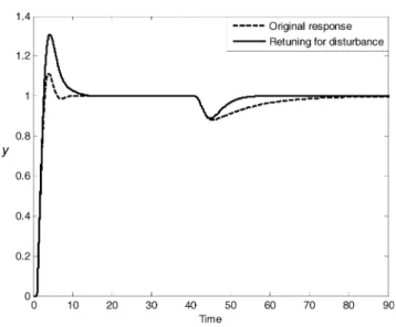
but sluggish disturbance response because the (Am, φm) pair

satis-fies eq 12 and is away from the curve in Figure 3. The closed-loop response as shown in Figure 9 demonstrates this expected result. Better disturbance response can be achieved if we retune the PID controller based on specifications given in Figure 3. By choosing Ms) 1.8, the specifications are found as A*m ) 2.5

and φ*_m) 41°. The value of R in eq 24 is chosen as 0.25. The tuning procedure converges after one iteration of ∆ (∆(1) ₎

1.198), and the PID controller is obtained as

The actual gain and phase margins of this resulting control system are Am) 2.54 and φm) 42.8°. The closed-loop response

after retuning is also shown in Figure 9, where the disturbance response is much improved. However, the set-point response becomes not so satisfactory because of the control objective we aim to. This result indicates that the gain and phase margins are indeed related to the control performance so that the control objective should be taken into account when the controller is tuned to achieve user-specified gain and phase margins.

Example 3. Consider a high-order process and a PID

controller given by

The actual gain and phase margins are 1.70 and 23.8°, respectively. On the basis of the modified relay feedback, the estimated gain and phase margins are Am) 1.66 and φm)

22.7°, where the value of∆ converges after two iterations with ∆(0)_{) 0.820, ∆}(1)_{) 0.726, and ∆}(2)_{) 0.663.}

To improve the system performance, retune the PID controller according to the specifications of A*_m ) 3 and φ*_m ) 60°. Again, the value of R in eq 24 is chosen as 0.25. The results converge after two iterations of∆ (∆(2)_{) 2.999), and the PID}

controller is obtained as

The actual gain and phase margins of this resulting control system are Am) 3.04 and φm) 59.1°, which are very close to

the specified ones. For this process and the same specifications, the PID controller tuning proposed by Ho et al.9_{results in A}

m ) 3.38 and φm) 62.5°. Our proposed method can achieve the

specifications more closely. The closed-loop responses before retuning, after retuning, and by Ho et al.9_{are shown in Figure}

10. The proposed controller also has better performance than that of Ho et al.9

Example 4. Consider a process with RHP zero and a PI

controller, which are used for simulation by Ma and Zhu,7_given

by

For the cases ofβ ) 1 and β ) 0.1, the actual gain and phase margins together with the estimated values by Ma and Zhu7

and the proposed method are given in Table 3 for comparison. As is seen from Table 3, the proposed method can estimate the gain and phase margins more accurately than the method proposed by Ma and Zhu.7 _{The error between the actual and}

estimated phase margins by Ma and Zhu7_{is large for processes}

with RHP zero. Figure 8. Closed-loop responses of example 1 (θ ) 1.5).

Figure 9. Closed-loop responses of example 2.

G_c(s) ) 8.255

(

)

(

)

Figure 10. Closed-loop responses of example 3.

Table 3. Actual and Estimated Gain Margin and Phase Margin in Example 4

actual value estimated7 _{estimated (proposed method)}

β Ahm φhm Am φm Am φm ∆d) ∆(2) 1 1.28 20.0° 1.19 12.7° 1.20 16.5° 0.501 0.1 3.49 51.6° 3.29 41.8° 3.34 51.8° 1.789 G_c(s) ) 1.207

(

)

(

)

For the case of β ) 1, the gain and phase margins of the control system are too small to have reasonable performance. Thus, the PI controller is retuned by the proposed procedure with the specifications chosen as A*_m) 3 and φ*_m) 60°. These specifications are achieved after two iterations of∆ (∆(2) ₎

4.961), and the PI controller is obtained as

The actual gain and phase margins of this resulting control system are Am ) 3.22 and φm ) 60.3°. The closed-loop

responses before and after retuning are shown in Figure 11.

Example 5. Consider a 2× 2 Wood and Berry process given

by

The performance of multiloop PI controllers proposed by Loh et al.25_{as the following is assessed.}

The actual gain and phase margins calculated are given in Table 4. The modified relay feedback tests are conducted sequentially to estimate the gain and phase margins of two equivalent SISO loops. The procedure and estimated results are shown in Table 4. The numbers of iterations for the first and second loops are 2 and 4, respectively. The estimated values are close to the calculated ones, which indicates the proposed method is also effective for multiloop control systems. The set-point responses of this system are shown in Figure 12. The response of loop 1 is aggressive because of its lower gain and phase margins. However, the response of loop 2 is sluggish because its phase margin is very large.

To improve the control performance, retune gc2(s) first by

specifying A*_m,2) 2.2 and φ*_m,2) 70°for the second loop. The result converges after two iterations of∆2(∆2(2)) 10.49), and

gc2(s) is obtained as

The actual gain and phase margins of this resulting control system are Am,1) 2.07 and φm,1) 32.6°for loop l and Am,2)

2.21 and φm,2) 71.8°for loop 2. The gain and phase margins

of loop 2 are very close to the specified ones after retuning, while the gain and phase margins of loop 1 are similar to those before retuning. Then, retune gc1(s) by specifying A*m,1) 2.5

and φ*_m,1 ) 50°for the first loop. The result converges after one iteration of∆1(∆1(1)) 1.76), and gc1(s) is obtained as

Now, the actual gain and phase margins after retuning of two controllers are Am,1) 2.49 and φm,1) 53.2°for loop l and Am,2 ) 2.33 and φm,2 ) 73.1° for loop 2. They are close to the

specified ones. The closed-loop responses after retuning are shown in Figure 12. It is seen that the performance of loop 2 is improved after retuning of gc2(s) and that the performance of

loop 1 is improved after retuning of gc1(s). 7. Conclusions

A relay feedback based method for tuning a PI/PID controller with an assessment of gain and phase margins is proposed. The proposed method estimates the gain and phase margins for systems with unknown controller and process dynamics. The estimated results can be used to assess the performance of the closed-loop system. When the retuning of the controller is found necessary, the proposed method can be applied to tune the PI/ PID controller based on the user-specified gain and phase margins. Simulation results have shown that the proposed method is effective for processes with different kinds of dynamics and for multiloop systems. Performance assessment and controller tuning can be done by the same approach, which can ensure a good performance of the control system.

Literature Cited

(1) Ender, D. B. Process Control Performance: Not as Good as You Think. Control Eng. 1993, 40, 180.

Figure 11. Closed-loop responses of example 4 (R ) 1).

Table 4. Actual and Estimated Gain Margin and Phase Margin in Example 5 actual estimated loop Ahm φhm Am φm ∆(0) ∆(1) ∆(2) ∆(3) ∆(4) 1 2.07 33.5° 2.06 30.2° 0.785 0.752 0.690 2 2.18 89.9° 2.19 89.8° 2.659 3.102 24.69 15.69 19.67 G_c(s) ) 0.32

(

)

[

]

(

)

(

)

Figure 12. Closed-loop responses of example 5: (a) loop 1 set-point change

and (b) loop 2 set-point change.

g_c2(s) ) -0.076

(

)

g_c1(s) ) 0.771

(

)

(2) Harris, T. J.; Seppala, C. T.; Desborough, L. D. A Review of Performance Monitoring and Assessment Techniques for Univariate and Multivariate Control Systems. J. Process Control 1999, 9, 1.

(3) Ho, W. K.; Lim, K. W.; Hang, C. C.; Ni, L. Y. Getting More Phase Margin and Performance Out of PID Controllers. Automatica 1999, 35, 1579.

(4) Huang, H. P.; Jeng, J. C.; Chiang, C. H.; Pan, W. A Direct Method for Multi-loop PI/PID Controller Design. J. Process Control 2003, 13, 769. (5) Ho, W. K.; Hang, C. C.; Zhou, J. H. Performance and Gain and Phase Margins of Well-Known PI Tuning Formulas. IEEE Trans. Control

Syst. Technol. 1995, 3, 245.

(6) Ho, W. K.; Gan, O. P.; Tay, E. B.; Ang, E. L. Performance and Gain and Phase Margins of Well-Known PID Tuning Formulas. IEEE Trans.

Control Syst. Technol. 1996, 4, 473.

(7) Ma, M. D.; Zhu, X. J. Performance Assessment and Controller Design Based on Modified Relay Feedback. Ind. Eng. Chem. Res. 2005,

44, 3538.

(8) Åstro¨m, K. J.; Ha¨gglund, T. Automatic Tuning of Simple Regulators with Specifications on Phase and Amplitude Margins. Automatica 1984,

20, 645.

(9) Ho, W. K.; Hang, C. C.; Cao, L. S. Tuning of PID Controllers Based on Gain and Phase Margin Specifications. Automatica 1995, 31, 497.

(10) Wang, Y. G.; Shao, H. H. PID Autotuner Based on Gain- and Phase-Margin Specifications. Ind. Eng. Chem. Res. 1999, 38, 3007.

(11) Ho, W. K.; Lee, T. H.; Gan, O. P. Tuning of Multiloop Proportional-Integral-Derivative Controllers Based on Gain and Phase Margin Specifications. Ind. Eng. Chem. Res. 1997, 36, 2231.

(12) Tan, K. K.; Lee, T. H.; Wang, Q. G. Enhanced Automatic Tuning Procedures for Process Control of PI/PID Controllers. AIChE J. 1996, 42, 2555.

(13) Scali, C.; Marchetti, G.; Semino, D. Relay with Additional Delay for Identification and Autotuning of Completely Unknown Processes. Ind.

Eng. Chem. Res. 1999, 38, 1987.

(14) Chen, Y.; Hu, C.; Moore, K. L. Relay Feedback Tuning of Robust PID Controllers With Iso-Damping Property. Proceedings of the 42nd IEEE

Conference on Decision and Control, Hawaii, Dec. 2003; p 2180.

(15) Chiang, R. C.; Yu, C. C. Monitoring Procedure for Intelligent Control: On-Line Identification of Maximum Closed Loop Log Modulus.

Ind. Eng. Chem. Res. 1993, 32, 90.

(16) Li, W.; Eskinat, E.; Luyben, W. L. An Improved Autotune Identification Method. Ind. Eng. Chem. Res. 1991, 30, 1530.

(17) Wang, Q. G.; Hang, C. C.; Zou, B. Low-Order Modeling from Relay Feedback. Ind. Eng. Chem. Res. 1997, 36, 375.

(18) Huang, H. P.; Jeng, J. C.; Luo, K. Y. Auto-Tune System Using Single-Run Relay Feedback Test and Model-Based Controller Design. J.

Process Control 2005, 15, 713.

(19) Huang, H. P.; Jeng, J. C. Monitoring and Assessment of Control Performance for Single Loop Systems. Ind. Eng. Chem. Res. 2002, 41, 1297. (20) Hang, C. C.; Ho, W. K.; Cao, L. S. A Comparison of Two Design Methods for PID Controllers. ISA Trans. 1994, 33, 147.

(21) Huang, H. P.; Lin, F. Y. Decoupling Multivariable Control with Two Degrees of Freedom. Ind. Eng. Chem. Res. 2006, 45, 3161.

(22) Hang, C. C.; Åstro¨m, K. J.; Ho, W. K. Refinements of the Ziegler-Nichols Tuning Formula. IEE Proc. DsControl Theory Appl. 1991, 138, 111.

(23) Zhuang, M.; Atherton, D. P. Automatic Tuning of Optimum PID Controllers. IEE Proc. DsControl Theory Appl. 1993, 140, 216.

(24) Burrus, C. S.; Gopinath, R. A.; Guo, H. Introduction to WaVelets

and WaVelet Transforms; Prentice-Hall: Upper Saddle River, NJ, 1998.

(25) Loh, A. P.; Hang, C. C.; Quek, C. X.; Vasnani, V. U. Autotuning of Multiloop Proportional-Integral Controllers Using Relay Feedback. Ind.

Eng. Chem. Res. 1993, 32, 1102.

ReceiVed for reView November 24, 2005 ReVised manuscript receiVed March 27, 2006 Accepted March 31, 2006