領導型證券分析師所考量基本會計/非會計變數與所追蹤個股組合之實證研究

行政院國家科學委員會專題研究計畫 成果報告

領導型證券分析師所考量基本會計/非會計變數與所追蹤個

股組合之實證研究

中 華 民 國 93 年 3 月 30 日

領導型證券分析師所考量基本會計/非會計變數與所追蹤個股組合之

實證研究

Abstract

We identify lead and follow analysts based on the timeliness of their recommendations, documenting more pronounced market reactions to the buy/hold/sell ratings issued by the analysts who systematically provide their recommendations ahead of the others. In many ways, our methodology is similar to that of Cooper, Day, and Lewis (2001), who ranked analysts by the timeliness in their earnings forecasts. Nevertheless, it may be more challenging but equally as valuable to identify the leaders and followers among the analysts in terms of their recommendations.

I. Introduction

This study examines the capital market returns and volumes accompanying lead versus follow analyst recommendations. Our primary goal is to better understand the difference in the perceived information contents in the recommendations by these two groups of analysts. Prior papers documented the extent to which various characteristics of security analysts help explain the differences in market reactions to analysts’ research reports.1 In contrast, we aim at a systematic investigation in identifying the forerunners among the analysts via the timeliness of their recommendations, testing whether the analysts who systematically issue the

buy/hold/sell ratings ahead of the others are perceived as the ones with superior

ranking performance.

We identify lead and follow analysts based on the timeliness of their

1 _{See Clement and Tse (2003), who documented that there is an association between forecast accuracy}

as well as market response and analyst characteristics such as analyst experience, broker size, and the number of firms and industries the analyst follows, and thus induce market reaction. Also see Stickel (1995), who documented more pronounced market reactions to All-America Research Team analyst recommendations.

recommendations. In many ways, our methodology is similar to that of Cooper, Day, and Lewis (2001), who ranked analysts by the timeliness in making earnings forecasts. Both investment recommendations and earnings forecasts are the key elements in analysts’ research reports. Nevertheless, as compared with distinguishing the analysts who provide more timely estimates from the others, it may be a more difficult task for the market to recognize the forerunners for the buy/hold/sell ratings. Note that the audience recognizes the target year of each earning forecast measure and can easily find the analysts who provide the EPS estimates well before the report days. In contrast, it may require a systematic investigation in finding the forerunners in investment recommendations since the extent a firm is over- or under-priced changes incessantly. Even when there exists no new firm value-relevant events subsequent to an unbiased recommendation, a research report issued immediately afterwards may be informative when the market under- or over-reacts to prior analyst opinions. There are various drivers to an analyst’s issuing a recommendation. The emergence of value-relevant events, market inefficiencies, or the pressure for imitation may all trigger a recommendation with short lead-time but long follow-time2. Therefore, it may be more challenging but equally as valuable to identify the leaders and followers among the analysts in terms of their recommendations.

Furthermore, the clustering of analyst recommendations makes the research designs for such studies even more challenging.3 The capital market studies most typically focus on the corporate events such as dividend announcements, stock splits as well as acquisitions and test the market prices and volumes on specific days. In

2 _{We define lead (follow) time as the number of days preceding (following) each recommendation. See}

section II for more details.

examining market accompanying an analyst recommendation, nevertheless, one may under- or over-estimate the perceived information content if he regards each announcement, which may arrive close in time to the other analysts’ recommendations, as a stand-alone event. Accordingly, we hand-collect (1) the forerunning lead and follow analyst recommendations, which are issued at least 13 days after the most recent recommendations, and (2) the paired-up lead and follow analyst recommendations. Our findings on both groups are consistent with the notion that the market perceives the lead analysts as the superior price forecasters.

Our study may add to the literature in the following aspects. First, we develop the procedures to identify lead and follow analysts in making recommendations. Such measures differ in many aspects from the procedures for ranking analysts by the timeliness in making earnings forecasts. Second, we develop the procedures to identify the forerunning lead and follow groups as well as the paired-up lead and follow groups. Such designs aim to cope with the phenomenon in clustering of analyst recommendations. Third, we extend the studies of the perceived information contents. Prior studies evidenced that price reaction is a function of several characteristics of analysts (Stickel (1995); Clement and Tse (2003)). Gleason and Lee (2003) documented that analyst’s forecast conveys new information to the market when he revises his own prior and consensus forecast. In contrast, we examine the market reactions to the recommendations by the analysts with differential timeliness.

The remaining sections of this paper are organized as follows. Section II describes our data and sample selection. Section III presents our research designs and empirical results. We conclude the paper in Section IV.

We collected the analyst recommendations during 1994-2001 from First Call Database, which provides the real-time investment recommendations to its subscribers by coding 1 to 5 (1: Strong Buy, 2: Buy, 3: Hold, 4: Sell, 5: Strong Sell). In our 1994-2001 sample periods, there are more than 77,000 recommendations for more than 6,600 firms per year.

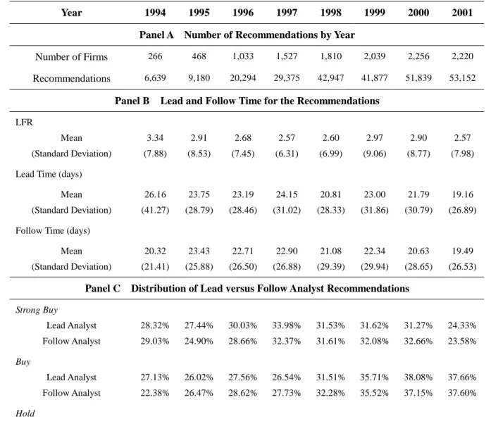
Our sample criteria are as follows. First, we select the firms with at least five different analyst recommendations in a given year. These five analysts have to give at least one recommendation to any stock each month in the previous year. Such criterion helps in reducing the error in identifying the lead analysts. Second, the firm’s market variables such as price and volume are available in the CRSP database. Table 1 (Panel A) provides the descriptive statistics on the number of matched observations by year.

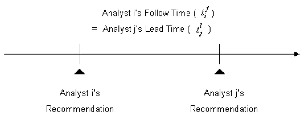
Our approach to identifying the lead and follow analysts is in a manner similar to that of Cooper et al. (2001), who identify lead and follow analysts in terms of the timeliness in making earnings forecast. Specifically, we calculate by hand the lead (follow) time, namely, the number of days preceding (following) a recommendation. Figure 1 illustrates the lead and follow time of analyst recommendations.

We then aggregate total lead time and total follow time, and calculate the lead-follow time ratio (LFR) as the total lead-time divided by the total follow time for each analyst-firm combination.

LFR =

∑

∑

where t_ikl and t_ikf are the numbers of days preceding and following the kth recommendation by analyst i, respectively. And K is the number of recommendations for the firm given by analyst i within a given year.

Table 1 Descriptive Statistics for Analyst Recommendations in 1994-2001

Year 1994 1995 1996 1997 1998 1999 2000 2001

Panel A Number of Recommendations by Year

Number of Firms 266 468 1,033 1,527 1,810 2,039 2,256 2,220

Recommendations 6,639 9,180 20,294 29,375 42,947 41,877 51,839 53,152

Panel B Lead and Follow Time for the Recommendations

LFR Mean (Standard Deviation) 3.34 (7.88) 2.91 (8.53) 2.68 (7.45) 2.57 (6.31) 2.60 (6.99) 2.97 (9.06) 2.90 (8.77) 2.57 (7.98)

Lead Time (days)

Mean (Standard Deviation) 26.16 (41.27) 23.75 (28.79) 23.19 (28.46) 24.15 (31.02) 20.81 (28.33) 23.00 (31.86) 21.79 (30.79) 19.16 (26.89) Follow Time (days)

Mean (Standard Deviation) 20.32 (21.41) 23.43 (25.88) 22.71 (26.50) 22.90 (26.88) 21.08 (29.39) 22.34 (29.94) 20.63 (28.65) 19.49 (26.53)

Panel C Distribution of Lead versus Follow Analyst Recommendations

Strong Buy Lead Analyst Follow Analyst 28.32% 29.03% 27.44% 24.90% 30.03% 28.66% 33.98% 32.37% 31.53% 31.61% 31.62% 32.08% 31.27% 32.66% 24.33% 23.58% Buy Lead Analyst Follow Analyst 27.13% 22.38% 26.02% 26.47% 27.56% 28.62% 26.54% 27.73% 31.51% 32.28% 35.71% 35.52% 38.08% 37.15% 37.66% 37.60% Hold

Lead Analyst Follow Analyst 40.59% 42.74% 42.20% 44.48% 39.53% 38.87% 36.86% 36.64% 33.95% 34.01% 30.06% 29.34% 29.03% 28.48% 35.25% 35.52% Sell Lead Analyst Follow Analyst 2.38% 3.43% 2.35% 1.91% 1.47% 2.23% 1.20% 2.42% 1.71% 1.47% 1.74% 2.01% 1.28% 1.31% 1.88% 2.43% Strong Sell Lead Analyst Follow Analyst 1.58% 2.42% 2.00% 2.24% 1.40% 1.62% 1.42% 0.83% 1.30% 0.63% 0.87% 1.05% 0.34% 0.40% 0.88% 0.87% Number of Analysts Lead Analyst Follow Analyst 44 54 81 83 109 118 138 134 147 150 174 173 183 176 177 187 Recommendations Lead Analysts Follow Analysts 505 496 1,403 1,205 2,924 2,596 4,235 3,837 5,906 5,378 6,104 5,515 7,054 6,618 7,512 6,878

Finally, we rank the analysts into five quintiles by LFR. We identify the analysts in the top (bottom) quintiles of LFR as the lead (follow) analysts for the firm. Namely, we identify for each firm its lead and follow analysts by this procedure.

Our methodology differs from that of Cooper et al. (2001) in the following ways. First, we adopt stricter standards to identify the forerunners in investment recommendations. Cooper et al. (2001) define an analyst as a leader if and only if his LFR exceeds one, whereas we identify the ones with LFR in the top (bottom) quintile as the lead (follow) analysts. Second, instead of using only one year to identify lead or follow analysts, our sample period ranges from 1994 to 2001. Such a design helps in reducing the error of wrong identifications. Third, we exclude the observations with none or only one recommendation in the previous or subsequent year.

Panel B of Table 1 summarizes both lead-time and follow-time for the recommendations. It indicates that the average follow-time for a recommendation is more stable; on the contrary, the range of lead-time is, with a wider variation, from 19 to 26 days throughout the sample period. Panel C of Table 1 reports the frequency of the lead versus follow analyst recommendations, demonstrating that that the lead (follow) analysts issue the recommendations more (less) frequently. Both lead and follow analysts tended to be more conservative before 1998 (the mode category is

hold), and seem to have become more optimistic after 1999 (the mode category is

buy). Also consistent with prior studies, both groups appear to be reluctant to make

sell recommendations.

III. Research Design and Test Results

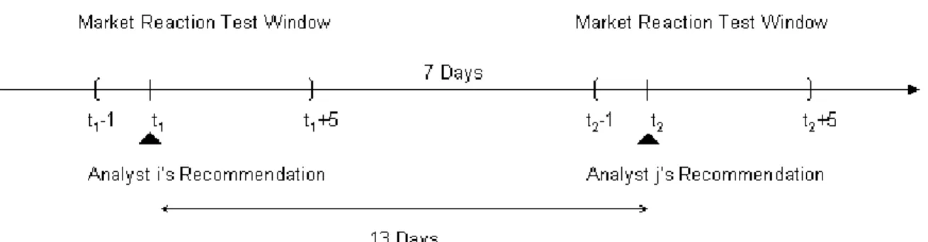
We form the forerunning leader or follower group of the recommendations which are at least thirteen days from the immediately prior recommendations. We then

examine the market reactions to lead versus follow analyst recommendations in short window [-1, +5]. As shown in Figure 2, on account of the early dissemination and delayed response issues, we require at least seven-days between two market reaction test windows.

We also hand-collect the observations with time interval between two lead analysts’ (or two follow analysts’) recommendations being within 13 days to form the paired-up leader (or the paired-up follower) groups. In each group of non-overlapping pairs, both former and latter recommendations are issued by the leaders (or followers). Moreover, there should be no leader recommendations (no follower recommendations) between two follower (two leader) recommendations.

Figure 2 The Market Reaction Test Window

We derive the market model mean-adjusted returns by subtracting the market model, which is estimated within the window from day -2 to day -256, expected returns from the corresponding raw returns. The seven-day buy-and-hold return for each observation is calculated as:

] 1 ) 1 ( [ ] 1 ) 1 [( ] 1 ) 1 ( [ 5 1 , 7 5 1 ,

∏

∏

t i

r, is the raw return on analyst-firm combination i on day t, rm,t is the return of

value-weighted CRSP market index, and

∧ ∧

i i β

α , are the coefficient estimates by using the market model.

Then, the mean of AR_iMean−Adjusted is calculated as:

Mean AR_iMean−Adjusted=1( ) 1

∑

where n equals the number of sample firms in the event period with available returns.

The market adjusted return is calculated as raw return minus the CRSP value-weighted index. The seven-day buy-and-hold return is calculated as:

] ) 1 ( ) 1 ( [ 5 1 , 5 1 ,

∏

∏

Likewise, we derive the mean of ARiMarket Adjusted −

.

Forerunning Lead versus Follow Analyst Recommendations

Table 2 presents the mean seven-day cumulative returns for forerunning leader and follower recommendations. Given the same criteria of lead-time, the key advantage to the design is to facilitate the comparison of the perceived ranking performance of lead versus follow analyst. We divide the recommendations into three categories: upgrades, downgrades, and reiterations.

The raw return is 1.99% (1.87%) and mean-adjusted return is 1.39% (1.05%) for upgrading lead (follow) analyst recommendations. Both are significant at 0.1%. Moreover, the market reaction is more significant for downgrading lead analyst recommendations. The corresponding mean-adjusted return is -2.48% (-1.44%) for lead (follow) analyst recommendations. As to the reiterations, the market reaction to the lead analyst recommendations appears to be negative.

Table 2 Market Reactions to Lead versus Follow Analysts by Recommendation Changes

7-day Mean Buy-and-Hold Return Lead Analyst Follow Analyst Comparison Test t-statistics

Upgrade

N Raw Return

Mean-Adjusted Return(Market Model)

Market Adjusted Return

3,990 1.99% (11.92)*** 1.39% (9.14)*** 1.67% (10.94)*** 3,582 1.87% (9.74)*** 1.05% (6.29)*** 1.33% (7.72)*** 0.47 1.51 1.48 Downgrade N Raw Return

Mean-Adjusted Return(Market Model)

Market Adjusted Return

4,095 -1.94% (-10.38)*** -2.48% (-15.17)*** -2.32% (-13.32)*** 3,578 -0.68% (-3.59)*** -1.44% (-8.68)*** -1.07% (-6.29)*** -4.74*** -4.47*** -5.13*** Reiteration N Raw Return

Mean-Adjusted Return(Market Model)

Market Adjusted Return

4,941 0.26% (1.67) -0.31% (-2.16)* -0.08% (-0.53) 4,535 0.54% (3.28)** -0.06% (-0.37) 0.19% (1.26) -1.24 -1.15 -1.27

The symbols *, **, and *** denote statistical significance at 5%, 1%, and 0.1%, respectively, using a 2-tailed test.

Volume ratio,VRi,t, for each recommendation is calculated as the ratio of the

volume,V_i,t, for each relative event day to the average volume from three months (60 trading days) before to three months after the event period.

120 / 1 * ) ( 66 7 , 66 7 , , ,

∑

∑

∑

where n is the number of firms; V_i,t is the volume for analyst-firm combination i at day t. 0.00% 50.00% 100.00% 150.00% 200.00% 250.00% -5 -4 -3 -2 -1 0 1 2 3 4 5 Trading Day (Event Day = Day 0)

V ol um e R atio Lead_Upgrade Lead_Downgrade Lead_Reit erat e Follow_Upgrade Follow_Downgrade Follow_Reit erate

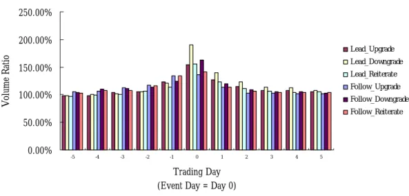
Figure 3 Abnormal Volume accompanying Lead versus Follow Analyst Recommendations

Figure 3 depicts the abnormal volume accompanying forerunning leader versus follower recommendations (event-day=day 0). The event-day trading volume is approximately 155% (191%) of the non-event-day average for the lead analysts’ upgrades (downgrades) against the immediately prior analyst recommendation. As for the follow analysts, the mean event-day volume is approximately 137% (162%) of the non-event-period average for analysts’ upgrades (downgrades). Nevertheless, for both

leader and follower groups, all of the volume ratios are statistically different from the one at the event date.

Table 3 presents the 3-day [-1, +1] mean volume ratios for both forerunning leader and follower recommendations. Except for the reiterations, the volume ratio for the lead (follow) analysts’ revisions appears to be more (less) pronounced.

Table 3 Three-Day Mean Volume Ratio for Lead versus Follow Analyst Recommendations

Recommendation Change

Lead Analyst Follow Analyst T-Test t-statistics

Wilcoxon Signed Ranks Test Z- statistics

Upgrade 134.57% 127.80% 3.08** 2.87**

Downgrade 150.42% 135.47% 4.79*** 2.30*

Reiteration 130.79% 129.63% 0.52 -1.08

The symbols *, **, and *** denote statistical significance at 5%, 1%, and 0.1%, respectively, using a 2-tailed test.

In sum, Tables 2 and 3 provide the evidence that the forerunning leader recommendations induce significantly greater market reactions.

Paired-up Lead versus Follow Analyst Recommendations

This section examines the market reactions to the ratings issued within 13 days after the most recent recommendation. For each pair of leader or follower recommendations, we define the event-day (day 0) as the day at which the latter analyst issues the recommendation. Furthermore, we calculate the volume ratio as the ratio of volume,V_i,t, to the mean daily volume from 60 trading days before to 60 trading days after the recommendation.

120 / 1 * ) ( 66 7 , 66 7 , , ,

∑

∑

where V_i,A_t(V_i,B_t) is the volume corresponding to the recommendation by the former (latter) analyst of the matched pair.

Table 4 reports the market reactions to the latter recommendations of the pairs. It indicates that the market reacts significantly to both the forerunning groups. Both mean-adjusted and market adjusted returns for upgrades are insignificant. In contrast, the subsequent lead analyst still has significant impact on the market when he downgrades prior lead analyst’s recommendation. The corresponding mean-adjusted return is -1.80% and the mean volume ratio is 164.10%. The market response appears to be significantly more negative than the latter of paired-up followers’. As for the reiterations, the difference between the two groups is insignificant. Consistently, in unreported analyses we find more pronounced price reactions to lead analyst recommendations in both Lead_ Lead versus Lead_ Follow and Follow_ Lead versus Follow_ Follow comparison tests.4

To further distinguish the market perceptions of the paired-up analyst recommendations, we document the market reactions by the magnitude of the changes in their recommendations. For the upgrades, we use the following four partitions: 1) buy to strong buy, 2) hold to buy and strong buy, 3) sell and strong sell to hold, and 4) sell and strong sell to buy and strong buy. We also use four partitions for downgrades: 1) strong buy to buy, 2) strong buy to hold, 3) buy to hold, and 4) strong buy, buy and hold to sell and strong sell. Furthermore, we categorize the reiterations into three groups: 1) strong buy, 2) buy, and 3) least favorable rating (including hold, sell, and strong sell). Table 5 presents the test results.

4_{First, the market model mean-adjusted returns accompanying the latter of the Lead_ Lead (Lead _}

Follow) pairs are more (less) significant. Second, the mean-adjusted returns accompanying the latter of the Follow_ Lead (Follow _ Follow) pairs are more (less) significant.

Table 4 Market Reactions to the Latter of the Paired Recommendations

Recommendation Change Lead_ Lead Follow_ Follow Comparison Test t-statistics Upgrade

N Raw Return

Mean-Adjusted Return(Market Model)

Market Adjusted Return

3-day Mean Volume Ratio

336 1.13% (1.13) 0.54% (0.99) 0.41% (0.79) 137.59% 259 0.86% (1.38) 0.47% (0.82) 0.12% (0.22) 134.43% 0.23 0.09 0.39 0.44 Downgrade N Raw Return

Mean-Adjusted Return(Market Model)

Market Adjusted Return 3-day Mean Volume Ratio

354 -1.75% (-3.45)*** -1.80% (-3.88)*** -2.13% (-4.73)*** 164.10% 268 -0.25% (-0.37) -0.39% (-0.61) -1.00% (-1.63) 130.87% -1.76+ -1.78+ -1.48 3.61*** Reiteration N Raw Return

Mean-Adjusted Return(Market Model)

Market Adjusted Return

3-day Mean Volume Ratio

404 -0.64% (-1.20) -1.01% (-1.98)* -1.11% (-2.25)* 154.89% 293 -0.88% (-1.25) -0.96% (-1.52) -1.18% (-2.00)* 149.02% 0.27 -0.06 0.09 0.46 The Lead_ Lead (Follow_ Follow) sample consists of the paired-up lead (follow) analyst recommendations.

The symbols +, *, **, and *** denote statistical significance at 10%, 5%, 1%, and 0.1%, respectively, using a 2-tailed test. The t-statistics in parentheses in columns 2 and 3 indicate whether the returns are significantly different from zero.

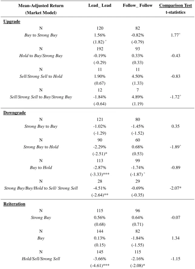
Table 5 demonstrates that market reactions to the disagreement between pairs of lead analysts are more pronounced. Probably due to the uncertainty, the more divergent the ratings within the pairs of recommendations, the more negative market reactions they would induce. When the revision is from strong buy to hold, the mean-adjusted return is -2.29%. As to the revision is from favorable ratings (strong buy, buy and hold) to less favorable ratings (strong sell and sell), the mean-adjusted return is -4.51%. Furthermore, the return is negative even for the upgrading recommendations from sell/strong sell to buy/strong buy.

The investors appear to react positively to upward revisions from buy to strong buy. The mean-adjusted return for the paired-up leader recommendations is 1.56%. Conversely, the signals from the other upgrades are insignificant, with all the mean-adjusted returns not reliably different from zero. Moreover, no matter whether up- or down-ward revisions are issued by the follower, the market appears to have no significant reactions. As for the reiterations of hold, sell, and strong sell, the latter recommendations appear to more significantly reinforce the investors’ negative beliefs. Specifically, the mean-adjusted return for the latter leaders who reiterate hold, sell, and strong sell is -3.66% and is significant at 0.1%.

Furthermore, we provide the test results for the comparisons between forerunning and paired-up lead analyst recommendations in Table 6. In terms of return and volume tests, the market reacts significantly to the paired-up reiterations. In spite of the statistical insignificance, the paired-up leader recommendations induce greater trading volume. The results suggest that the recommendation of the latter lead analyst recommendation has some impacts on the market.

Table 5 Market Reactions to Analyst Recommendations Arriving in Pairs Mean-Adjusted Return

(Market Model)

Lead_ Lead Follow_ Follow Comparison Test t-statistics Upgrade

N

Buy to Strong Buy

N

Hold to Buy/Strong Buy

N

Sell/Strong Sell to Hold

N

Sell/Strong Sell to Buy/Strong Buy

120 1.56% (1.82) + 192 -0.19% (-0.29) 11 1.90% (0.67) 12 -1.84% (-0.64) 82 -0.82% (-0.79) 93 0.33% (0.33) 11 4.50% (1.33) 7 4.89% (1.19) 1.77+ -0.43 -0.83 -1.72+ Downgrade N

Strong Buy to Buy

N

Strong Buy to Hold

N

Buy to Hold

N

Strong Buy/Buy/Hold to Sell/ Strong Sell

121 -1.02% (-1.29) 90 -2.29% (-2.51)* 113 -2.87% (-3.33)*** 28 -4.51% (-2.64)** 80 -1.45% (-1.52) 60 0.68% (0.53) 99 -1.74% (-1.87) + 29 -0.69% (-0.35) 0.35 -1.89+ -0.89 -2.07* Reiteration N Strong Buy N Buy N Hold/Sell/Strong Sell 115 0.56% (0.68) 144 0.13% (0.15) 145 -3.66% (-4.61)*** 96 0.64% (0.71) 82 -1.84% (-1.55) 115 -2.16% (-2.08)* -0.07 1.34 -1.15

The symbols +, *, **, and *** denote statistical significance at 10%, 5%, 1%, and 0.1%, respectively, using a 2-tailed test

The t-statistics in the parentheses in columns 2 and 3 indicate whether the returns are significantly different from zero.

Table 6 Comparison Tests for the Forerunning Lead versus Latter of the Paired-up Lead Analyst Recommendations

Panel A 7-day Mean-Adjusted Return Lead_ Lead Lead Analyst Comparison Test t-statistics Upgrade 0.54% 1.39% -1.50 Downgrade -1.80% -2.48% 1.38 Reiteration (All) -1.01% -0.31% -1.32 Reiteration (Sub-samples) Strong Buy N

7-day Mean-Adjusted Returns

Buy

N

7-day Mean-Adjusted Returns

Hold/Sell/Strong Sell

N

7-day Mean-Adjusted Returns

115 0.56% 144 0.13% 145 -3.66% 1,427 1.52% 1,647 -0.60% 1,867 -1.46% -1.11 0.81 -2.67** Panel B 3-day Mean Volume Ratio Lead_ Lead Lead Analyst T-Test

t-statistics

Wilcoxon Signed Ranks Test Z- statistics

Upgrade 137.59% 134.57% 0.58 2.65** Downgrade 164.10% 150.42% 1.63 4.08*** Reiteration 154.89% 130.79% 2.65** 4.57***

The Lead_ Lead sample consists of the paired-up lead analyst recommendations.

IV. Conclusion

Our goal in this paper is to investigate the perceived information contents of lead versus follow analyst recommendations. First, we identify lead and follow analysts based on the timeliness of their recommendations and examine the market reactions to the forerunning leader or follower recommendations. Second, we examine the market reactions accompanying the pairs of lead or follow analysts.

Our result is consistent with the notion that the lead analysts invoke greater market reactions than the follow analysts. First, the price impacts of the forerunning leader (follower) recommendations appear to be more (less) pronounced. Moreover, the event-day volumes accompanying upgrading and downgrading recommendations are approximately 155% and 191% of the non-event-day average, respectively.

Second, for the buy/hold/sell ratings arriving in pairs, the market has positive reactions when the latter lead analysts consistently issue favorable recommendations. However, the market reactions are more negative if there exists divergence between the pairs of lead analyst recommendations. Moreover, the market reactions to the paired-up follower recommendations are insignificant. In sum, our results indicate that the market reactions to the lead (follow) analyst recommendations are more pronounced for both fore-running and paired-up groups.

References

Barber, Brad, Reuven Lehavy, Maureen McNichols, and Brett Trueman, 2001, Can investors profit from the prophets? Security analyst recommendations and stock returns, Journal of Finance 56 (2), 531-563.

Clement, Michael B. and Senyo Y. Tse, 2003, Do investors respond analysts’ forecast revisions as if forecast accuracy is all that matters? The Accounting Review 78 (1), 227-249.

Cooper, Rick A., Day Theodore E., Lewis, Craig M., 2001, Following the leader: a study of individual analysts’ earnings forecasts, Journal of Financial Economics 61, 383-416.

Gleason, Cristi A., Charles M. C. Lee, 2003, Analyst forecast revisions and market price discovery, The Accounting Review 78 (1), 193-225

Stickel, Scott E., 1995, The anatomy of the performance of buy and sell recommendations, Financial Analysts Journal 51, 25-39.

Welch, Ivo, 2000, Herding among security analysts, Journal of Financial Economics 58, 369-396. Womack, Kent L., 1996, Do brokerage analysts’ recommendations have investment value? Journal of Finance 51 (1), 137-167.