Failure Modeling and Process Monitoring for Flexible
Manufacturing Systems Using Colored Timed
Petri Nets
Chung-Hsien Kuo and Han-Pang Huang
Abstract—The performance of a flexible manufacturing system
(FMS) depends on the equipment efficiency and process control. In order to increase the equipment efficiency, the failure mode anal-ysis and fault diagnosis can be used to reduce the frequency of unexpected breakdowns of machines. In addition, the statistical process control (SPC) can be used for adjusting the process pa-rameters to eliminate process variations. In this paper, a colored timed Petri net (CTPN) is used to model the process behavior of an FMS. In addition, the CTPN-based SPC, fault diagnosis, and failure model and effect analysis are modeled and analyzed indi-vidually. Especially, all of the modular models are integrated and linked based on the CTPN. Due to the unified CTPN modeling, the information of each modular model in the entire system can be exchanged and integrated directly and efficiently. Finally, the entire CTPN FMS models are implemented using G2 real-time ex-pert system. Consequently, the proposed CTPN-based simulator can be acted as a real-time FMS monitor and controller through the G2 standard interface.
Index Terms—CTPN, fault diagnosis, FMEA, FMS, SPC.
I. INTRODUCTION
T
HIS PAPER proposes the failure modeling and process monitoring for a flexible manufacturing system (FMS) using a colored timed Petri net (CTPN). Such an approach aims to integrate necessary components for an FMS together using a unified modeling methodology. The process status and data can be generated from the CTPN real-time simulator, and they can be analyzed to improve system performance using the statistical process control (SPC), failure model and effect analysis (FMEA), and fault diagnosis.Petri nets (PN’s) [4], [21] can model the concurrent and asyn-chronous components in systems using graphical and mathe-matical methodologies. Initially, it is used to discuss the munication between the asynchronous components of a com-puter system. Several literatures used the traditional PN or mod-ified PN to model an FMS. Among these, Zhou et al. [25] pre-sented a flexible manufacturing cell construction using a PN mathematical model. Jeng [12] proposed a PN synthesis theory for modeling FMS’s. Abdallah et al. [1] proposed an efficient search algorithm for deadlock-free scheduling in an FMS using
Manuscript received September 3, 1998; revised June 3, 1999 and February 1, 2000. This paper was recommended for publication by Associate Editor A. Kohhar and Editor P. Luh upon evaluation of the reviewers’ comments. This work was supported in part by the National Science Council, Taiwan, under Grant NSC85-2212-E-002-073 and Grant NSC85-2622-E-002-018.
The authors are with the Robotics Laboratory, Department of Mechanical Engineering, National Taiwan University, Taipei 10660, Taiwan, R.O.C.
Publisher Item Identifier S 1042-296X(00)05727-X.
a PN. Zhou et al. [27] used the PN to generate the optimal con-trol policy for flexible manufacturing cells. Hu et al. [6] used a generalized stochastic PN to model and analyze an FMS for scheduling and control decision support system applications. Hence, a PN is selected in this paper to model the FMS. Since the behaviors of the FMS are very complex, the operation time and resource color attributes are critical for analysis. The time attribute characterizes the efficiency of the equipment. The re-source attribute (color set) characterizes different types of prod-ucts and machines. Hence, a CTPN [14]–[17] was developed based on the traditional PN, adding the time property and color attribute. In addition, the proposed CTPN is designed in a mod-ular, object-oriented, and hierarchical configuration.
The reliability of the automated equipment influences the per-formance of the FMS directly. However, highly reliable devices cost much more. Correct and rapid fault diagnosis can reduce the mean time to repair (MTTR) and improve the efficiency of the equipment. On the other hand, the SPC can be used to identify the cause defects for eliminating process variations. Especially, the breakdown of machines and out-of-control process affect the dispatching system since some resources are not available for a period of time. The components in an FMS are intercorrelated and interdisturbed dynamically. They must be modeled and an-alyzed using a consistent methodology to ease the coupling ef-fects. Hence, the integrated modeling approach of SPC, FMEA, fault-diagnosis, dispatching, and process models using CTPN’s is required.
In this paper, the activities in an FMS are imbedded in multi-level structures [14]–[17], that is, production, process, cell, and machine levels. The proposed hierarchical structure was devel-oped from the layered architecture for factory coordination (FC) and production activity control (PAC) proposed by [3]. Finally, the proposed CTPN models are applied to an FMS at the Man-ufacturing Automation Technology Research Center (MATRC) of National Taiwan University. In addition, the proposed FMS simulator is developed on a real-time and object-oriented expert system G21 [5]. GSI (G2 standard interface) and GFI (G2 file interface) are used concurrently.
II. FMS’S ANDMODELING
A. FMS’s
An FMS [14] consists of a number of systems, such as process actions, material handling devices, material storage, 1G2 is developed by Gensym Corporation, Cambridge, MA 02140 USA. It is
a real-time and object-oriented expert system. 1042–296X/00$10.00 © 2000 IEEE
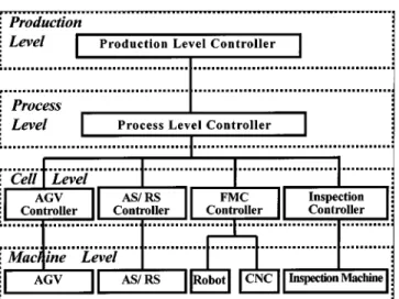
Fig. 1. Hierarchical structure of the FMS.
control units, inspection stations, and gauging stations. The ma-terial flows among the flexible manufacturing cells, machines, and equipment are often connected through an automated material handling system. Production control messages, in-cluding process information, product information, and control commands are routed via a communication system. The com-munication system is composed of computers, control units, and a local area network [14], [22]. The FMS can manufacture mixed products in variable and small batch sizes. In addition, the flexible route, process, machine, etc., meet fast transition of customer requirements and deliver the products in a timely fashion. Hence, an FMS has the ability to cope with rapid market and demand changes.
In this paper, the FMS is decomposed into the following four levels [14]–[17]: production level, process level, cell level, and machine level, as shown in Fig. 1. This architecture is devel-oped based on a layered architecture for FC and PAC proposed in [3]. This control architecture is similar to the National In-stitute of Standards and Technology (National Bureau of Stan-dards)—Automated Manufacturing Research Facility (CIM ar-chitecture). In addition, the International Standard Organization (ISO) provides a reference model (ISO, 1984 [11]) for the trans-formation between different architectures. The production level is the highest level in an FMS and manages the FMS opera-tions. It includes the master production schedule, system re-source management, databases, maintenance, and system per-formance measurement. The process level coordinates and con-trols all cells in the FMS, for example, the real-time scheduling (dispatching) system. The cell level is the manufacturing cell level below the process level. Finally, the machine level may be composed of machining devices, inspection devices, and mate-rial handling equipment, such as conveyors, machining centers, lathe machines, milling machines, inspection centers, robots, and automatically guided vehicles (AGV’s).
In addition, the dispatching of an FMS is critical. In this research, 13 rules [14] are used. The dispatching rules can be based on either workpieces or machines. The rules based on workpiece characteristics are as follows: 1) first come first served; 2) shortest processing time (SPT); 3) weighted SPT; 4) shortest remaining processing time; 5) longest remaining
liest finishing time with alternative considered; 5) LITA+ESTA (combination of LITA and ESTA).
B. CTPN
A CTPN is a type of PN. The color attributes [4], [9], [14]–[17] manage large systems that have many similar or redundant logical structures. The time attribute [4], [14]–[17] allows various time-based performance mea-sures to be conducted in the system model. A time-delay can be assigned to either places or transitions to model the time elements in a system. A CTPN is tentuple, , where is a set of timed places, is a set of timed transitions, is a set of immediate places, is a set of immediate transitions, is a set of communication places, is a set of macro transitions, is a set of directed arcs, is a set of inhibitor arcs, is a set of interrupt arcs, is the color set of transitions and places. The detailed definitions, properties, and enabled conditions of the CTPN can be referred to [14]. Briefly, the components of the CTPN are described below.
The immediate places describe the conditions or properties (without time factor) of resources. The timed places describe the time properties of resources. The communication places describe the communication packages in a CTPN. The com-munication and interface between the macro transitions are conducted through four types of communication places. The pitch-down and catch-down places are applied to higher level modules; the pitch-up and catch-up places are for lower level modules. The higher level modules use pitch-down places to send (or pitch) tokens to lower level modules. The catch-down place is used to receive (or catch) tokens from lower level modules. Similarly, the lower level modules use the pitch-up places to send tokens to the higher level modules. The catch-up place catches tokens from the higher level modules [14].
The immediate transitions describe the behaviors or events (without time factor) of resources. The timed transitions describe the time properties of resources. The macro transitions are often used to formalize a modular design [18], [24]. A macro transition is the combination of a series of transitions, places, and arcs. The interconnection between different levels is achieved by communication places. Based on macro transitions and communication places, a hierarchical and modular model of the FMS can be constructed. The directed arc connects a place to a transition, or vice versa. A place connected with an inhibitor arc is called an inhibitor place. When an inhibitor place contains the same color token as the output transition, the output transition is inhibited to fire. Similarly, a place con-nected with an interrupt arc is called an interrupt place. When an interrupt place contains the same color token as the output transition, the firing of the output transition is interrupted and further inhibited. For an immediate transition, the interrupt and
Fig. 2. Icon definition of CTPN graph.
the inhibitor arcs behave the same. For a timed transition, if the timed transition is firing and the interrupt place has the same color, then it interrupts the firing of this transition and returns the color token to the input place(s) [14]. The icon definition of CTPN is shown in Fig. 2. These elements are further elaborated as follows [14].
1) Place: is a finite set of places,
, including immediate places, timed places, and communication places. Notice that the immediate places describe the conditions or properties (without time factor) of resources. The timed places describe the time proper-ties of resources. The communication places describe the communication packages in a CTPN.
2) Transition: is a finite set of
tran-sitions, , including immediate transitions, timed transitions, and macro transitions. Notice that the imme-diate transitions describe the behaviors or events (without time factor) of resources. The timed transitions describe the time properties of resources.
3) Color: and represent the color sets of
places in and transitions in
where and are nonnegative integers, and are colors of places and transitions, and denotes the car-dinality.
4) Input, output, inhibitor, and interrupt functions: , is an input function. It describes the mapping relation from the transition with color to the place with color , where is an nonnegative integer. Similarly, , is an output
function. , is
an inhibitor function. , is an interrupt function.
5) Marking: , has
el-ements. is an vector defined as
, where is the number of
tokens of colors at this instant; is the total number
of colors in place ; denotes the number of
tokens of colors in place ; is the initial marking. 6) Conditions of enabling and firing: The transition is
en-abled with respect to the color if
After the transition is fired, two outcomes could appear. For an immediate transition, the new marking becomes
For a timed transition, the temporary marking is
After the delay in , the marking becomes
7) Time function: It is simply the time attribute in the places and transitions. For the transition,
is the time required by the timed transition associated with the color to complete the firing. For the place, is the time delay required in the timed place associated with the color to release. 8) Reachability set: It consists of all reachable markings
from the initial marking. Reachability is a basic property of the CTPN. A marking is said to be reachable from the initial marking if there exists a sequence of firings that transforms to . The firing sequence (FS) is de-noted by
where to
is the color set of the transition
9) Liveness, deadlock [26]: For any reachable marking, if there exists a firing sequence of transitions to reach a marking and enable transition , then the transition is live. A CTPN is live if all transitions in the net are live. For any reachable marking, if there is no firing sequence of transitions to make enable, then the transition is dead-locked. A CTPN is deadlocked if there exist no transitions in the net to be enabled.
An FMS CTPN production model [7], [14] can be constructed as follows: 1) analyze the FMS; 2) define the system require-ments, resources, decision-makings, and events; 3) use macro transitions to model the cells and machines; 4) define the pro-cesses in terms of material flow or machines in different levels; 5) draw flow charts of the processes; and 6) define the interface
Fig. 3. Relationship between SPC and process.
and communication between different levels and macro transi-tions; 7) use CTPN to model the flow charts in step 5); 8) val-idate the constructed CTPN model. In addition, the CTPN ele-ments must be related to the physical components in an FMS. These relationships can be referred to [14].
III. CTPN-BASEDSPC
A. Operation of Process Control in an FMS
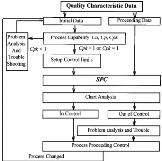
Quality control, management, and integration have been more emphasized in recent years [2], [10], [19], [20]. However, quality control and management systems cannot stand alone. They must be analyzed using collected data, and then the result is used to control the process and prevent defects. When process conditions change, the process parameters must be adjusted according to process variability. SPC can be used to investigate and control the process, as shown in Fig. 3. SPC [13] is based on statistics and is widely used for process control to improve product quality, eliminate process variability, and isolate the causes of defects.
In this paper, process control includes the process capability and the SPC. Initially, the process capability is validated. If the process capability is acceptable, then the control limits of the SPC can be generated to investigate process variability. If any measurement is reasoned to be out of control, then the causes of defects are identified. Consequently, the corresponding process parameter is adjusted to correct the process. The flow of process control is illustrated in Fig. 4. In this paper, a control chart of the SPC tools [20] is used to validate the process.
B. CTPN-Based SPC Model
The SPC activities in this paper are constructed in terms of CTPN. Two major functions of the process control, including process capability and SPC, are modeled as macro transitions. Since the value of each measurement is not the same, the tradi-tional PN cannot handle attribute-based measurement. For ex-ample, the SPC macro transition can generate results (such as one measurement is out of three times of standard deviation) for incoming (different value) measurement. The SPC activities in Fig. 4 can be converted into a CTPN, as shown in Fig. 5. The CTPN elements in this CTPN-based SPC net are described as follows. SPC_P1 represents the data collected from the shop floor. SPC_T1 indicates the initial data collection, and SPC_T2 indicates the subsequent data collection. SPC_T1 and SPC_T2 are controlled and mutually excluded by SPC_P2. The number
Fig. 4. Application of SPC activities in the FMS.
of tokens in SPC_P2 indicates the required initial number for an-alyzing the capability of the process. If a token exists in SPC_P2, then SPC_T2 is inhibited. SPC_T6 represents the capability analysis of the process.
The process capability is used to characterize the process ca-pability with respect to the standard specification of the process. In this paper, the process capability can be evaluated in terms of the precision capability , accuracy capability , and process capability index [20]. SPC_P5 contains the data analyzed by the process capability. SPC_T3 and SPC_T4 are controlled by the color set of the tokens in SPC_P5, and they represent the incapable and capable processes, respectively. If a process is analyzed as incapable, then SPC_P6 restarts the ca-pability analysis of the process after adjusting the process pa-rameters.
If the process is capable, then SPC_T11 is not inhibited, and the subsequent measurements are analyzed using the SPC module, i.e., SPC_T7. In this net, the SPC module is imple-mented using a control chart. Control charts are widely used in SPC. SPC_P11 stores the results of the control chart analysis. These results are identified in terms of “in control” and “out of control.” SPC_T8 represents “in control,” and SPC_T9 represents “out of control.” The inhibitor arc connected to SPC_T2 is designed for controlling the number of initial data measurements for analyzing the process capability. There is a specified number of tokens (depends on the process capability and initial measurement requirement) in SPC_P2 in the initial marking. If there still exist tokens in SPC_P2, then SPC_T2 is inhibited when a measurement (colored token) is collected from SPC_P1. If there is no token in SPC_P1, then SPC_T1 will be not enabled, and SPC_T2 will be enabled when a measurement enters SPC_P1. In addition, the inhibitor arc connected to SPC_T6 implies when the initial measurements are complete, the process capability can be executed to generate the indices of process capability. Consequently, the inhibitor arc connected to SPC_T11 indicates if the process capability is not acceptable,
Fig. 5. Modeling SPC using CTPN.
Fig. 6. Modeling machine fault and maintenance.
then SPC_T7 contains token(s), and hence inhibits the enabling of SPC_T11 and the operation of SPC module.
IV. CTPN-BASEDFAILUREMODEL ANDFAULTDIAGNOSIS
A. CTPN-Based Failure and Preventive Maintenance Models
The performance of a machine depends on its availability. In this paper, the CTPN model for machine layer includes the machining process, maintenance, and failure behaviors. An ex-ample of CTPN failure and maintenance model for a machining center (MC) is shown in the right-hand side of Fig. 6. In this net, MC_T2 represents the machining of MC. When an MC is ma-chining, it may be interrupted (and sequentially inhibited) by a sudden failure or inhibited by the preventive maintenance (PM). MC_P11 represents the sudden failure of machine from sensor
detection or the “out-of-control” status of the process from the SPC CTPN net. MC_P12 represents the PM of the MC. Either PM, process out of control, or failure leads the stoppage, rep-resented by MC_P13, and MC_P16 records this message. Es-pecially, MC_P17 sends this message to the fault diagnosis and FMEA CTPN’s to find the cause problem and failure models. When the cause problem is found, the maintenance is started (MC_P18). The time to repair (MC_T9) depends on the color set of the fired token. Different types of PM, failure, and process parameter adjustment lead to different time elapsed in MC_T9. Notice that the elapsed time is determined by the MTTR gener-ally.
MC_P14 and MC_P15 indicate the status of failure and PM, respectively. If the machine has been repaired, then MC_P23 will receive this token. The token in MC_P23 cooperates with
(a) (b)
(c) (d)
Fig. 7. Transformations of CTPN and fault tree for FMEA. (a) AND gate. (b) OR gate. (c) Condition gate. (d) Order AND gate.
token(s) in MC_P14 or MC_P15 to enable MC_T8 (failure is repaired) or MC_T7 (PM is finished), respectively. Therefore, the uses of the interrupt and inhibitor arcs can be designed to control the enabling/firing of MC_T2. Since the time to repair in MC_T9 requires the classification of failure modes, and the processing time of MC_T2 depends on the incoming product attributes, the ordinary PN is not suitable here.
B. CTPN-Based FMEA and Fault Diagnosis Models
Fault diagnosis is important since it affects the machine uti-lization, system performance, and costs. Usually, the FMEA and the fault diagnosis are analyzed in terms of individual system. In this paper, the fault diagnosis and FMEA are constructed in terms of CTPN’s so that information can be exchanged directly. A fault tree [23] can be used to analyze the failure modes and effects. It can also be used to identify various possible failure modes and effects. A fault tree constructs the structural form of failures, and its simple logical relationships represents the probabilistic relationships among various events that lead to the failure of a system. Based on the logical relationships, the CTPN and the fault tree can be mapped into each other.
The analysis of a fault tree requires related component status collected from the corresponding sensors. For example, the analysis of a hydraulic system requires the tank status from a level gauge and the pump status from a pressure gauge. In this paper, a sensor-based configuration is used to construct the fault tree. In order to convert the fault tree into the CTPN model, the events are defined as follows:
1) on–off sensors—modeled by traditional PN;
2) analog sensors—measurement value of the analog sensor is divided into appropriate levels, e.g., the value of level
gauge can be classified into the hihigh, high, normal, low, and lolow levels.
Due to the hierarchical and modular configuration of the CTPN, the fault tree can be modeled hierarchically. The CTPN elements can be directly mapped to their corresponding fault tree elements. Some important fault tree symbols that relate to the FMS are selected in this paper, such asANDgates,ORgates, condition gates, order AND gates, basic events, intermediate events, and transfer events. The transformation is described as follows.
1) Events are modeled by places. 2) Gates are modeled by transitions.
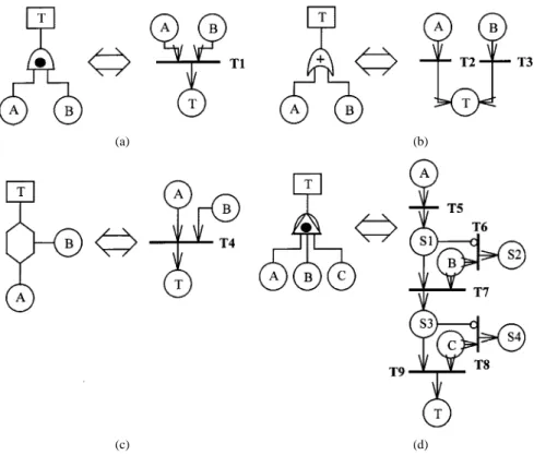
3) Complex systems, such as an FMS’s, are modeled by hi-erarchical and modular configuration.
Based on the transformation between the CTPN and the fault tree, the converted CTPN models can be used for FMEA and fault diagnosis. When the FMEA is used, the conversion be-tween the elements of the fault tree and CTPN can be illustrated in Fig. 7. In this figure, A, B, and C are sensor measurements, T is the event of failure, S1, S2, S3, and S4 are used for sequen-tial control. T1 to T9 are the transitions. In Fig. 7(a), theAND
gate is transformed. From the viewpoint of FMEA, the failure of A and B causes the failure of T. Hence, the converted CTPN model can be constructed in the right-hand side of Fig. 7(a). In Fig. 7(b), theORgate is transformed. From the viewpoint of
FMEA, the failure of A or B causes the failure of T. Hence, the converted CTPN model can be constructed in the right-hand side of Fig. 7(b). The condition gate in Fig. 7(c) can also be con-structed. In Fig. 7(d), the order gate is transformed. From the viewpoint of FMEA, the failure of T is caused from the ordered failures of A then B and C. Hence, the converted CTPN model uses inhibitor arcs connected to T7 and T8 to denote that the
(a) (b)
(c) (d)
Fig. 8. Transformations of CTPN and fault tree for fault diagnosis. (a) AND gate. (b) OR gate. (c) Condition gate. (d) Order AND gate.
Fig. 9. Example of fault tree application.
failure of T is caused from the component failure sequence of A B C. If the failure sequence is not A B C, then T9 is never fired. For example, if B occurs before A, then the token in place B is delivered to place S2. When A occurs sequentially, the token in A will not be sent to S3 because the token in place B is removed.
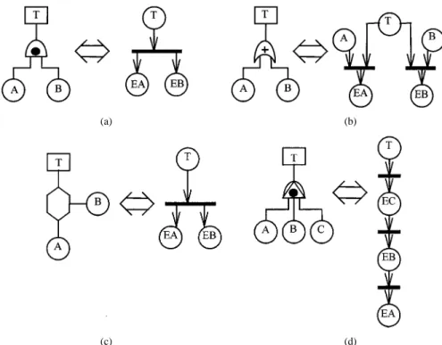
In addition to the FMEA analysis, this paper also proposes the CTPN-based fault diagnosis. When the fault diagnosis is used, the conversion between the elements of the fault tree and the CTPN can be illustrated in Fig. 8. In Fig. 8, A, B, and C are sensor measurements, and T is the event; EA, EB, and EC are the diagnosis results, and they correspond to the sensors of A,
Fig. 10. CTPN-based FMEA model of fault tree in Fig. 9.
B, and C. In Fig. 8(a), theANDgate is transformed. From the viewpoint of fault diagnosis, if T is failed, then both A and B must be failed, too. Hence, the converted CTPN model can be constructed in the right-hand side of Fig. 8(a). In Fig. 8(b), the
ORgate is transformed. From the viewpoint of fault diagnosis, if T is failed, then either A or B must be failed. Hence, the con-verted CTPN model can be constructed in the right-hand side of Fig. 8(b). Similarly, the “condition” and “order” gates are con-structed in Fig. 8(c) and (d), respectively.
Fig. 11. CTPN-Based fault diagnosis model of fault tree in Fig. 9.
Fig. 12. CTPN integrated manufacturing environment.
In order to illustrate those transformations practically, a fault tree example is used to illustrate the transformations from the fault tree to the FMEA and the fault diagnosis CTPN models, as shown in Fig. 9. In this figure, T is a top event for describing a system failure. B1 to B6 are the intermediate events that are caused by a combination of other events via a fault tree logic gate. G0 to G6 are fault tree logic gates. A1 to A8 are basic failure components in the system. The transformations of FMEA can be done from Fig. 7. Fig. 10 shows the trans-formation from a fault tree in Fig. 9 to a CTPN FMEA model. In this figure, the symbols T, G , and A are related to the events in the fault free of Fig. 9. In addition, A is a place that has the same attributes with A . Notice that the symbols of and are nonnegative integers. Besides, the areas circled by the round rectangle line are components of the fault tree logic gates. From the CTPN firing rules [14], if the components A7 and A3 are failed, then tokens in places A7 and A3 form an
Fig. 14. Integration of CTPN model, process control, and monitoring.
place T. It can be concluded that from the viewpoint of FMEA, the failures of A7 and A3 cause the failure of T.
The transformations of fault diagnosis can also be done from Fig. 8. Fig. 11 shows such a transformation from a fault tree in Fig. 9 to a CTPN fault diagnosis model. In this net, the symbols T, G , and A are related to the events of the fault free in Fig. 9. In addition, A and B are message duplicates from A and B , respectively. Notice that the symbols of and are non-negative integers. EA indicates the failure of its corresponding component. For example, the status from the sensors are the components of A1, A7, and B1, which are working, A3 and A6, which are failed. Initially, the analysis starts from the FMEA analysis. From Fig. 10 of the FMEA analysis, the components of B2 and B5 must be failed. Then, the CTPN-based fault diag-nosis is used to find the major failure components that cause the system failure. After several firing sequences, only EA6 (among EA1 to EA8) has one token. This implies that component A6 is the major failure component that leads to the system failure.
V. APPLICATIONS
The proposed CTPN-based production, SPC, FMEA, and fault diagnosis are applied to an FMS at the Manufacturing Automation Technology Research Center (MATRC) of Na-tional Taiwan University. These components can be integrated as shown in Fig. 12. In this integrated CTPN architecture,
Fig. 15. Process capability analysis.
the communication places act as interfaces among modules. The FMS CTPN-based production models were proposed in [14]. The FMS at MATRC is composed of two flexible manufacturing cells (FMC’s), an automatically guided system (AGV), an automated storage/ retrieval system (AS/RS), and a coordinate measuring machine (CMM). The first FMC is composed of a CNC milling machine, a CNC lathe machine, a robot, and two buffers. The second FMC is a machining center. Fig. 13 shows the layout of the FMS.
In this paper, the CTPN-based FMS SPC, FMEA, and fault diagnosis models are constructed using G2 [5] real-time expert
Fig. 16. Control chart.
system. This real-time expert system supports GSI, GFI, and G2 Oracle Bridge (database). Based on the G2 interfaces, the FMS real-time simulator can communicate with the cell controller and database through the TCP/IP protocol. Hence, this CTPN-based FMS simulator can be used to control and monitor shop floor activities. The production information and quality measurement are stored in the database. The centralized CTPN-based FMS monitoring and control system communicates with the windows-based cell controllers through the TCP/IP protocol. The cell controller controls the equipment through the serial communication (RS/232). Due to the mod-ular design, the real-time simulator can be acted as a real-time monitor and controller.
The CTPN simulator [8] can also be transformed to a real-time dispatcher. Basically, the G2 rules can be used to infer the firing of the CTPN models from the initial conditions (markings). The firing sequences and reachable markings are recorded in the database (using G2 Oracle Bridge) or the text file (using G2 GFI interface). In the simulation stage, the dispatching rules are used to evaluate the system performance, such as the utilization of machines, due date for each batch, and bottlenecks. If the simulation result of a dispatching rule fits the manufacturing requirements, then the firing sequences can be worked as a dispatching order.
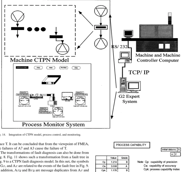
On the other hand, the proposed CTPN models are con-structed using a hierarchical and modular configuration. The model integration and information exchange of each module can be achieved in terms of communication places. Fig. 14 shows the relationships among CTPN models, shop floor con-trol, and process monitoring. In this figure, the key factor is the communication places that switch operation between simulator and controller. If communication places communicate with
Fig. 17. Example of fault tree of system layer.
the machine CTPN models, then the simulation environment is established. If communication places communicate with machine controller through the GSI, then the process control environment can be constructed. Especially, the modular design makes flexible combinations of the CTPN models, monitoring system, and dispatching system possible.
The process capability analysis is shown in Fig. 15. In this case, the values of , , and are acceptable. In addition, the control chart is used to examine process variation. Fig. 16 shows an X-Rm chart at which x-ucl, x-cl, and x-lcl are the upper control limit, central line, and lower control limit of the X-chart, respectively. In addition, a fault tree of the system layer in the FMS is shown in Fig. 17. The corresponding FMEA anal-ysis and fault diagnosis CTPN models are shown in Fig. 18. In this figure, REL_FMS_P1 to REL_FMS_P5 are the status col-lected from control, production, inspection, storage, and AGV systems. On the other hand, DIAG_FMS_P1, DIAG_FMS_P3, DIAG_FMS_P5, DIAG_FMS_P7, and DIAG_FMS_P9 are the status collected from the cell layer. They indicate the status col-lected from control, production, inspection, storage, and AGV systems. Consequently, the CTPN-based FMEA and fault diag-nosis models for each cell and machine can be constructed in
Fig. 18. Example of CTPN-based FMEA and diagnosis in Fig. 17.
the same manner. The entire FMS FMEA and fault diagnosis models can be integrated through the communication places.
VI. CONCLUSIONS
This paper uses a newly developed CTPN to model the ac-tivities of production, SPC, process failure, FMEA, and fault diagnosis in an FMS. Especially, the conversion between the fault trees and the CTPN models is used to analyze the FMEA and the fault diagnosis. The process control behaviors including process capability and SPC are also modeled in terms of CTPN. Based on these approaches, a complete FMS model can be con-structed using a unified modeling technology. Such research in-creases the integrability of models with different behaviors. In addition, the interactions and information exchanges among the activities of production, SPC, and process failure can be directly described and linked using CTPN. Due to the modular construc-tion, the CTPN models can be used to simulate and control the FMS concurrently through communication places. Most man-ufacturing systems with complex product mixes and flexible routes can be modeled, analyzed, and controlled in this manner using the proposed integrated CTPN modeling environment.
REFERENCES
[1] I. B. Adballah, H. EIMaraghy, and T. EIMekkawy, “An efficient search algorithm for deadlock-free scheduling in FMS using Petri nets,” in
Proc. EEE Int. Conf. on Robotics and Automation, vol. 2, Leuven,
Bel-gium, May 1998, pp. 1793–1798.
[2] A. L. Arentsen, J. J. Tiemersma, and H. J. J. Kals, “The integration of quality control and shop floor control,” Int. J. Comput. Integr. Manufac., vol. 9, no. 2, pp. 113–130, 1996.
[3] A. Bauer, R. Bowden, J. Browse, J. Duggan, and G. Lyons, Shop Floor
Control System—From Design to Implementation. London, U.K.: Chapman & Hall, 1991.
[4] A. A. Desrochers and R. Y. AI-Jaar, Applications of Petri Net in
Manufacturing Systems—Modeling, Control, and Performance Anal-ysis. New York: IEEE Press, 1995.
[5] Gensym Corporation, G2 Ref. Manual Version 4.0, Cambridge, MA, 1995.
[6] G. H. Hu, Y. S. Wong, and H. T. Loh, “An FMS scheduling and control decision support system based on generalized stochastic Petri net,” Int.
J. Adv. Manufac. Technol., vol. 10, pp. 52–58, 1995.
[7] H. P. Huang and P. C. Chang, “Specification, modeling and control of a fleexible manufacturing cell,” Int. J. Prod. Res., vol. 30, no. 11, pp. 2515–2543, 1992.
[8] H. P. Huang and Y. H. Tseng, “Modeling and graphic simulator for in-tegrated manufacturing systems,” Intell. Automat. Soft Computing, vol. 1, pp. 183–186, 1994.
[9] P. Huber, K. Jensen, and R. M. Shapiro, “Hierarchies in colored Petri nets,” in Advanced in Petri Nets 1990, Lecture Notes in Computer
Sci-ence. New York: Springer-Verlag, 1990, pp. 313–341.
[10] G. B. Hutchins, Introduction to Quality, Management, Assurance and
Control. New York: Macmillan, 1991.
[11] ISO International Standard 7498: Information Processing
Sys-tems—Open Systems Interconnection Basic Referencel Model, UDC,
681.3.01, ISO 7498-1984(E), 1984.
[12] M. D. Jeng, “A Petri net synthesis theory for modeling flexible man-ufacturing systems,” IEEE Trans. Syst., Man, Cybern. B, vol. 27, pp. 139–183, Apr. 1997.
[13] D. L. Kimbler and B. A. Sudduth, “Using statistical process control with mixed parts in FMS,” in Proc. JAPAN/USA Symp. on Flexible
Automa-tion, vol. 1, 1992, pp. 441–445.
[14] C. H. Kuo, H. P. Huang, and M. C. Yeh, “Object-oriented approach of MCTPN for modeling flexible manufacturing systems,” Int. J. Adv.
[17] C. H. Kuo, H. P. Huang, K. C. Wei, and S. S. H. Tang, “Dispatching and simulation for highly model-mixed automotive plants,” in Proc. Int.
Conf. on Automation Technology, vol. 1, Hsinchu, Taiwan, 1996, pp.
423–430.
[18] S. S. Lu and H. P. Huang, “Modularization and properties of flexible manufacturing systems,” in Advances in Factories of the Future, CIM
and Robotics, M. Cotsaftis and F. Vernadat, Eds. Amsterdam, The Netherlands: Elsevier, 1993, pp. 289–298.
[19] R. E. McQuater, B. G. Dale, R. J. Boaden, and M. Wilcox, “The effec-tiveness of quality management tools and techniques: An examination of the key influences in five plants,” Proc. Inst. Mech. Eng., vol. 210, pp. 329–339, 1996.
[20] D. C. Montgomery, Introduction to Statistical Quality Control, 2nd ed. New York: Wiley, 1990.
[21] T. Murata, “Petri nets: Properties, analysis and applications,” Proc.
IEEE, vol. 77, pp. 541–580, Apr. 1989.
[22] P. G. Ranky, Computer Integrated Manufacturing—An Introduction with
Case Studies. London, U.K.: Prentice-Hall, 1986.
[23] S. S. Rao, Reliability-Based Design. New York: NcGraw-Hall, 1992. [24] C. J. Tsai and L. C. Fu, “Modular approach for Petri-nets modeling of flexible manufacturing systems adaptable to various task-flow re-quirement,” Proc. IEEE Int. Conf. on Robotics and Automation, pp. 1043–1048, 1992.
[25] M. C. Zhou, K. McDermott, P. A. Patel, and T. Tang, “Construction of Petri nets based mathematical models of an FMS cell,” in IEEE Int. Conf.
on Systems, Man, and Cybernetics, 1991, pp. 367–372.
[26] M. C. Zhou and K. Venkatesh, Modeling, Simulation, and Control of
Flexible Manufacturing Systems—A Petri Net Approach. River Edge, NJ: World Scientific, 1999.
[27] Q. Zhou, M. Wang, and S. P. Dutta, “Generation of optimal control policy for flexible manufacturing cells: A Petri net approach,” Int. J.
Adv. Manufac. Technol., vol. 10, pp. 59–65, 1995.
of Hydraulic Control System at An-Feng Steel Company., Kaohsiung, Taiwan, R.O.C. From 1997 to 1998, he served as a technical consultant at Axon Technology Company, Taipei, Taiwan, R.O.C.. Cur-rently, he is an Assistant Professor at the Mechanical Engineering Department of Tung-Nan Junior College of Technology, Shen-Keng. His research interests include control systems, automation, software engineering, and ERP.
Han-Pang Huang graduated from National Taipei
Institute of Technology, Taipei, Taiwan, R.O.C., in 1977, and received the M.S. and Ph.D. degrees in electrical engineering from The University of Michigan, Ann Arbor, in 1982 and 1986, respec-tively.
Since 1986, he has been with the National Taiwan University, where he is currently a Professor in the Department of Mechanical Engineering. He was the Vice Chairperson of the Mechanical Engineering Department from August 1992 to July 1993 and the Director of Manufacturing Automation Research Technology Center, National Taiwan University, from August 1996 to July 1999. His research interests include machine intelligence, network-based manufacturing systems, intelligent robotic systems, prosthetic hands, and nonlinear systems.
Dr. Huang is a member of Tau Beta Pi, SME, CFSA, and CIAE. He was the Editor-in-Chief of the Journal of Chinese Fuzzy System Association and the Pro-gram Chair of the 1998 International Conference on Mechatronic Technology (ICMT’98). Currently, he is the Editor-in-Chief of the International Journal of
Fuzzy Systems. He has received two Distinguished Research Awards from the