Distribution of porous colloidal particles in an energy field

(1)

Distribution of porous colloidal particles in an energy field

Jyh-Ping Hsu

a,)

_{, Ming-Tsan Tseng}

a

_{, Shiojenn Tseng}

b

a

Department of Chemical Engineering, National Taiwan UniÕersity, Taipei, 10617, Taiwan, ROC

b

Department of Mathematics, Tamkang UniÕersity, Tamsui, Taipei, 25137, Taiwan, ROC

Received 28 July 1998

Abstract

The spatial distribution of colloidal particles in an energy field is evaluated theoretically. The field may be established by a relatively large object such as a rigid wall, a closed boundary, and a particle. The set of nonlinear hypernetted chain equations describing the variations of the correlation functions for particle–particle and particle–object interactions is solved. A numerical scheme based on the discrete Fourier transform is proposed for the former, and a Newton–Raphson iterative method for the latter. Three cases are examined to illustrate the method proposed, namely, particles in a planar slit, cylindrical pore, and square duct. The qualitative behavior of the spatial variation of the concentration of colloidal particles

w

predicted by the present study is consistent with that observed experimentally by D.H. Van Winkle and C.A. Murray J.

Ž . x

1. Introduction

If a suspension of colloidal particles is placed in an energy field, the dispersed particles will follow a certain distribution as a response to the applied field. The energy field can be generated, for instance, by a rigid wall, or by relatively large nearby entities

w_{1–4 . The phenomenon under consideration has po-}x

tential applications in various problems in practice. For example, knowing the distribution of colloidal particles in an electrolyte solution is essential to the estimation of the long-range depletion force between

w x

two relatively large particles 5–8 . The distribution coefficient, which is a function of the distribution of colloidal particles, plays a significant role in

exclu-w x

sion chromatography 9,10 .

)

Corresponding author. E-mail: [email protected]

Relevant studies are ample in the literature. Van

w x

Winkle and Murray 1 , for example, observed exper-imentally the spatial distribution of the concentration of monodispersed latex particles under the influence of a smooth repulsive glass wall. It was found that the concentration of particles decreases oscillatory

w x

away from the surface. Gonzalez-Mozuelos et al. 2 considered the distribution of colloidal particles in a planar slit. The one-dimensional problem was solved by applying a rescaled mean spherical approximation to calculate the direct correlation function between two particles, and a hypernetted chain approximation to evaluate the radial distribution function between particle and wall. The result derived was found to be similar to that obtained through a Monte Carlo

simu-w x

lation. In a subsequent study 3 , they also used a rescaled mean spherical approximation to estimate the radial distribution function, and concluded that the result obtained is close to that based on the

Ž .

(2)

hypernetted chain approximation. The analysis was extended to the problem of the adsorption of

parti-w x

cles to a planar slit 4 . It was proposed that if the concentration of colloidal particles is low, their dis-tribution can be approximated by the Boltzmann

w x

distribution 5,6 . However, since the volume of a colloidal particle is neglected, this assumption may lead to some deviation in the prediction of the

w x

behavior of a colloidal dispersion. Ise et al. 11 and

w x

Ito et al. 12 , for instance, concluded that, if the volume of a colloidal particle is considered, the Coulombic force between two particles having the same electrical property can be attractive. In a study of the attractive interaction between similarly charged

w x

colloidal particles, Chu and Wasan 13 found that, if the concentration of colloidal particles is high, and the amount of charges on the surface of a particle is large, the variation of the effective pair interaction energy as a function of the center-to-center distance between two particles can be oscillatory. At an ele-vated particle concentration, the distribution coeffi-cient of colloidal particles can be estimated by

adopt-w x

ing a Virial expansion technique 5,6,9,10,14 . In this approach, the distribution coefficient is expanded in an infinite power series of the bulk concentration of colloidal particles. The coefficients of the series are calculated through integrating the Mayer function

w x

associated with the cluster diagrams 9,14 . If some of these diagrams are neglected, the resultant integra-tion leads to either the Percus–Yevick approxima-tion, or the hypernetted chain approximation. In practice, since the coefficients of higher-order terms involve a complicated multiple integration, the corre-sponding terms are usually dropped for simplicity. One of the possible approaches to avoid this diffi-culty is to solve simultaneous integral equations based on the hypernetted chain approximation. This approach is often adopted to determine the distribu-tion of ions in an electrical double layer.

Lozada-w x

Cassou 15 , for example, used the hypernetted chain approximation associated with a mean spherical ap-proximation to calculate the distribution of ions near a cylindrical electrode. It was shown that, if the linear size of an ion is infinitely small, and the radius of the electrode approaches infinity, the result re-duces to that predicted by the Gouy–Chapman

the-w x w x

ory 16 . Zaini et al. 17 used the same approach to evaluate the distribution of ions in a cylindrical pore.

A bridge function was proposed to correct the devia-tion arises from the negligence of some of the graphs

w x

in the cluster diagram. Yeomans et al. 18 discussed the distance of ions within and surrounding a charged cylindrical pore by adopting a hypernetted chainr mean spherical approximation approach. It was con-cluded that the result obtained differs both quantita-tively and qualitaquantita-tively from that based on the Pois-son–Boltzmann theory, especially for small pores.

w x

Greathouse and McQuarrie 19,20 discussed the

electrical interaction force between two charged pla-nar surfaces. A variational method was adopted to solve the hypernetted chain equations. In a study of the electrical interaction between two charged

sur-w x

faces, Patey 21 solved a set of three hypernetted chain equations. Lozada-Cassou and co-workers

w_{22–24 suggested using a three-point extension hy-}x

pernetted chain method to improve the performance

w x

of the method proposed by Patey 21 .

Reported theoretical analyses in the literature are mainly of one-dimensional nature. While the result derived in this limited domain provides valuable information, a systematic analysis in a higher-dimen-sional space is highly desirable for practical

consid-w x

erations 1 . This is done in the present work. One of the key problems which needs to be solved in this case is the treatment of the set of equations govern-ing the spatial variation of particle concentration. The analysis is based on a hypernetted chain approx-imation, and an efficient solution procedure pro-posed. Three representative examples, namely, parti-cles in a planar slit, a cylindrical pore, and a square duct, are discussed.

2. Modeling

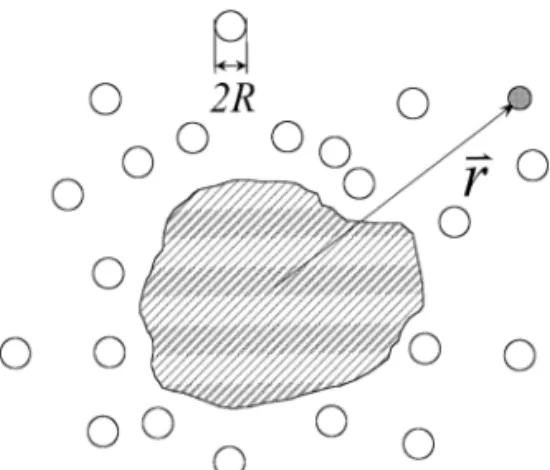
The system under consideration is illustrated in Fig. 1 where monodispersed colloidal particles with scaled radius R, represented by open circles, are dispersed in an electrolyte solution, and the shaded area denotes a rigid object. The concentration of colloidal particles follows some distribution as a response to the presence of the object. The object can be a rigid wall, a closed boundary, or a relatively large particle having a concentration much dilute than that of the colloidal particles. The density

(3)

distri-Fig. 1. Schematic representation of the system under consideration where the open circles represent the colloidal particles and the shaded area a relatively large object. R is the radius of a colloidal

©

particle, and r the scaled vector from the gravity center of the object to that of a particle.

©

Ž .

bution of colloidal particles, r r , can be expressed

w x as 25 : © © r r s r g

Ž .

` wc

Ž .

r ,

Ž .

1 © Ž .

where r` and gwc r are, respectively, the bulk

number concentration and the radial distribution of colloidal particles. The subscripts w and c denote the rigid object and the colloidal particle, respectively,

©

and r the scaled vector from the gravity center of the former to that of the latter which is scaled by the factor ry1 r3_{, i.e.,}

` © 1r3

r s rr` ,

Ž

1a

.

r being the center-to-center vector connecting object and colloidal particle. For the system shown in Fig.

Ž .

1, gwc r can be determined by the Ornstein–

w x Zernicke equations 25 : X X X hcc

Ž .

r s ccc

Ž .

r q

_H

hcc

Ž

r c

.

cc

Ž

r y r

.

d r ,

Ž

2a

.

V X X X hwc

Ž .

r s cwc

Ž .

r q

_H

hwc

Ž

r c

.

cc

Ž

r y r

.

d r , V 2b

Ž

.

with g s 1 q h ,i j i j i , j s w, c .

Ž

2c

.

Ž . Ž .

The integrations in Eqs. 2a and 2b are conducted

Ž . Ž .

over the space, and ci j r and hi j r are,

respec-tively, the direct and indirect correlation functions

between entities i and j, i, j s w, c. The derivations

Ž . Ž .

of Eqs. 2a and 2b are based on the assumption that the concentration of w is low. Employing the

w x

hypernettted-chain approximation 25 , we have c_{i j}

_{Ž .}

r s h_{i j}

_{Ž .}

r y ln 1 q h_{i j}

_{Ž .}

r y_u_{i j}

_{Ž .}

_{r ,}

i , j s w, c ,

Ž .

3

Ž .

where ui j r is the scaled, paired potential energy

Ž . Ž . Ž .

between entities i and j. Eqs. 2a , 2b and 3 lead

to two independent problems. First, given rcc and

u , we have to solve the following equations for hcc cc

and c :cc

hcc

Ž .

r s ccc

Ž .

r q hcc

Ž .

r ) ccc

Ž .

r ,

Ž

4a

.

c

_{Ž .}

r s h

_{Ž .}

r y ln 1 q h

_{Ž .}

r y_u

_{Ž .}

_{r ,}

_Ž

_4b

_.

cc cc cc cc

where the asterisk symbol denotes the convolution

operator. Second, given c_cc and u_wc, we have to

solve the following equations for h_wc and c_wc:

hwc

Ž .

r s cwc

Ž .

r q hwc

Ž .

r ) ccc

Ž .

r ,

Ž

5a

.

c_wc

_{Ž .}

r s h_wc

_{Ž .}

r y ln 1 q h_wc

_{Ž .}

r y_u_wc

_{Ž .}

_{r .}

5b

Ž

.

For convenience, we assume that colloidal particles

are spherical. In this case, both hcc and ccc are

functions of the distance between two particles only, and the vector r can be replaced by its magnitude r.

w x

The method proposed by Broyles et al. 26 is

Ž . Ž .

adopted to solve Eqs. 4a and 4b . The first step is

w _.

to extend the domain of hcc and ccc from 0, ` to

Žy_{`, ` by defining}.

x

h_cc

_{Ž .}

r s h_cc

_Ž

y_{r ,}

_.

_{r g y `, 0 ,}

_Ž

_6a

_.

x

c

_{Ž .}

r s c

_Ž

y_{r ,}

_.

_{r g y `, 0 .}

_Ž

_6b

_.

cc cc Also, we define H s r h y ccc

Ž

cc cc

.

,

Ž

7a

.

G s yrhcc cc,

Ž

7b

.

I s yrc s H y rhcc cc cc cc,

Ž

7c

.

r J s ycc

H

I s d s .

Ž .

Ž

7d

.

y` Ž . Ž .

Therefore, Eqs. 4a and 4b can be rewritten as

` X X X Hcc

Ž .

r s 2 p

_H

Icc

Ž

r

.

Jcc

Ž

r y r

.

d r y` ` X X X y

_H

_H_cc

_Ž

_r

_.

_J_cc

_Ž

_{r y r}

_.

_{d r} _,

_Ž

_8a

_.

y` h s y1 q exp H rr y ucc

Ž

cc cc

.

Ž

8b

.

(4)

For a simpler numerical treatment, these expressions are transformed to the corresponding discrete forms as N X X H s_{2 pd}

_Ý

_I _J Ž . cc , n cc , n cc , nyn X n syN N X y

_Ý

_H _J _,

_Ž

_9a

_.

Ž . cc , n cc , nyn X n syN h s y_{1 q exp H}

_Ž

r_{nd y u}

_.

_,

_Ž

_9b

_.

cc , n cc , n cc , n

where d is a discretizing interval, N an integer

< <

sufficiently large such that H_{cc, N}f_{0 for} _{n ) N,}

Ž .

and F the corresponding discrete form of F r i.e.,n

Ž .

F s F nd . The following iterative procedure isn

Ž . Ž .

used to solve Eqs. 9a and 9b :

Step 1. Guess an initial Hcc, n and substitute it into

Ž .

Eq. 9b to evaluate hcc, n.

Ž .

Step 2. Substitute h_{cc, n} into Eq. 7c , and the

Ž .

resultant expression into Eq. 7d to obtain I_{cc, n}

and J_{cc, n}.

Ž .

Step 3. Substitute I_{cc, n}and J_{cc, n} into Eq. 9a , and

take a discrete Fourier transform to obtain

ˆ

2 p Icc , kJcc , k

ˆ

H s _, y_{` - k - ` ,}

_Ž

₁₀

_.

cc , k

_ˆ

1 q 2 p Jcc , k

ˆ

where F is the Fourier transform coefficient of_k

F ._n

Step 4. Take the inverse Fourier transform on

ˆ

H_{cc, k} to obtain H_{cc, n}, and substitute the resultant

Ž .

expression into Eq. 9b to obtain the corrected hcc, n. The procedure is repeated until Hcc, n con-verges.

Ž .

F n can be recovered from Fn by choosing an

appropriate interpolation method. A linear interpola-tion approximainterpola-tion is used in the present study. It

Ž . Ž . Ž . Ž .

can be shown that Hcc t , Icc r , Jcc r , Gcc r are

< <

negligible for r G L. Typically, L is on the order of six radii of a colloidal particle.

Ž . Ž .

Note that in Eqs. 5a and 5b , hwc and cwc are

functions of vector r, and not functions of scalar r.

For a two-dimensional problem, we expand hwc and

c_wc as hwc

Ž .

r s

Ý

hwc , nN r , rn

Ž

n

.

, n s 1, 2, . . . ,

Ž

11

.

n cwc

Ž .

r s

Ý

cwc , nN r , rn

Ž

n

.

, n s 1, 2, . . . ,

Ž

12

.

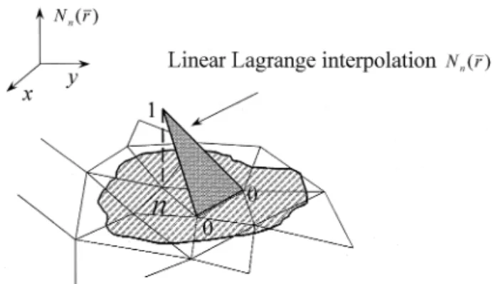
n Ž .

Fig. 2. Meshes used in the linear Lagrange interpolation of N r .n

where n is a mesh node shown in Fig. 2, hwc, n the

Ž . Ž .

value of hwc r at n, and N r, rn n an interpolation

function, r being the vector pointing to node n. Onen

of the interpolation functions often adopted is the linear Lagrange interpolation function, the property of which is shown in Fig. 2. This approach was used in a finite-element method to solve a variational

w x w x

problem 27 . It was also used by Zaini et al. 17 in the discussion of the double layer profile in a charged

Ž . Ž .

cylindrical pore. Substituting Eqs. 11 and 12 into

Ž . Ž .

Eqs. 5a and 5b and letting the residuals vanish at the nodes, we obtain

< < X X X h s_c q

_Ý

_{w h} _c

_˜

_Ž

_{r y r}

_.

_, wc , n wc , n n wc , n cc n n X n n s 1, 2, . . . ,

Ž

13a

.

c s_h y_{ln 1 q h}

_Ž

_.

y_u _, wc , n wc , n wc , n wc , n n s 1, 2, . . . ,

Ž

13b

.

where w is a weighting factor, which reflects then

integral of interpolation functions over the area occu-pied by node n by all mesh elements enclosing node n, and c

˜

cc is defined as ` 2 2

'

c

˜

cc

Ž .

r s

_H

ccc

_Ž

r q z

_.

d z .

Ž

14

.

y` Ž . Ž .

Note that Eq. 13a is linear and Eq. 13b nonlinear algebraic equations. The former can be rewritten as

(5)

Ž . Ž <

where the i, j element of matrix M is w cj

˜

cc r yi

<. r , andj hwc , 1 hwc , 2 h s _,

_Ž

_15a

_.

wc _h wc , 3 . . . c_{wc , 1} cwc , 2 c_wcs _.

_Ž

_15b

_.

cwc , 3 . . . Ž . Ž .

Substituting Eq. 15 into Eq. 13b gives

h s y_{1 q EXP Mh} y_{u ,}

_Ž

₁₆

_.

wc

ž

wc

/

where uwc , 1 uwc , 2 u_wcs _,

_Ž

_16a

_.

uwc , 3 . . . exp x

Ž

1

.

exp x

Ž

2

.

EXP x s

Ž

.

Ž

16b

.

exp x

Ž

3

.

. ._. Ž .

Eq. 16 is solved by the Newton–Raphson method through using the iterative expression

´ ´ ´ h s_h y_{S y1 q EXP ´ Mh} y_u wc Ž kq1. wc Ž k .

ž

wc Ž k . wc

/

´ y_h _,

_Ž

₁₇

_.

wc Ž k . ´

where h_{wcŽ k .} is the k th iterative solution with

param-eter ´ , 0 - ´ F 1, and S s M m EXP ´ Mh

_ž

y_u

_/

Ž . wc k wc

ž

= y₁

w

_{111 PPP 1}

x

y_I

_/

_.

_Ž

₁₈

_.

The operator m has the property

w

_a

x

m _b s

w

_c

x

_, _{c s a b .}

_Ž

_18a

_.

i j i j i j i j i j i j

The parameter ´ is designed to improve the perfor-mance of the present numerical scheme, which con-sists of the following steps:

Step 1. Assign a small value, say 0.1, to ´ , and assume the initial guess

´

h_{wc Ž0.}s_{EXP yu}

_Ž

_wc

_.

y_{1 .}

_Ž

₁₉

_.

Ž .

Step 2. Substitute this expression into Eq. 17 ,

and evaluate h´wcŽ1.. Repeat this step until a

con-´

vergent expression, hwcŽ`., is obtained.

Step 3. Increase the value of ´ , use h´wcŽ`. as the

initial guess, and return to step 1. This is repeated until ´ reaches unity.

3. Results

Three examples are discussed to illustrate the applicability of the present method. These include colloid particles in a planar slit, a cylindrical pore, and a square duct. The rectangular meshes shown in Fig. 3 are used in all these problems. According to Fig. 3, we have

w s Ar4 ,n

Ž

20

.

where A is the area of the mesh which encloses node n.

The distribution of colloidal particles depends on the energies of colloidal–colloidal and colloidal–ob-ject interactions. In the following discussions all the length scales are scaled by the inverse Debye length

(6)

k . A general expression for the colloidal–colloidal Ž . w x interaction energy, ucc r , is 5,6 ucc

Ž .

r exp y r y R y R

Ž

1 2

.

y₁ s_{4 p´ ´ k}_r ₀ _{R R Y Y}₁ ₂ _{1 2} _, r 21

Ž

.

where subscripts 1 and 2 denote the properties of

particles 1 and 2, respectively, ´ and ´r 0 are the

relative permittivity of the liquid phase and the permittivity of a vacuum, respectively, r is the scaled

center-to-center distance between two particles, R isi

the scaled radius of particle i, and Y is the scaledi

surface potential of particle i. Here we assume that the permittivity of the solid phase is much smaller than that of the liquid phase, as is usually the case in practice.

The interaction energy between colloidal particle and wall depends on their shapes and surface condi-tions. Suppose that it can be estimated through the linear superposition. Then, for the case of constant charge density, the interaction energy can be evalu-ated by

1 0 1 0

uwc

Ž .

r s W r HC2 c w d S q W r HC2 w c d S ,

Ž

22

.

where W s ´ ´ k Trk er 0 B 2, kB and T are,

respec-tively, the Boltzmann constant and the absolute

tem-perature, e is the elementary charge, r and rc w are,

respectively, the scaled surface charge densities of a

particle and the wall, Cw0 and Cc0 are the scaled

surface potentials of an isolated wall and an isolated particle, respectively.

Ž

As an example, we consider porous

ion-penetra-.

ble particles, which simulate a wide class of col-loidal particles, such as biological cells and particles

covered by an artificial membrane. In this case, Y ,_i

Ž .

i s 1, 2, in Eq. 21 should be replaced by the scaled

potential at particle–liquid interface, and r in Eq.c

Ž22 denotes the scaled volume charge density. It can.

be shown that for an ion-penetrable particle,

0

C_c

_{Ž .}

_{r s r exp y r y R}_c

_Ž

_.

_{R y 1}

q_{exp y2 R}

_Ž

_{. Ž}

_{R q 1}

_.

r_{2 r ,} _{r G R ,}

23

Ž

.

where R is the radius of the particle, and the interac-tion energy between two ion-penetrable spheres is

2 ucc

Ž .

r s W prc exp R

Ž

. Ž

R y 1

.

2 q_{exp yR}

_Ž

_{. Ž}

_{R q 1}

_.

_{exp yr rr .}

_Ž

_.

24

Ž

.

3.1. Planar slit

Consider a planar slit with a scaled width 2 L. Let R be the scaled radius of a particle. The origin of the

Ž .

coordinates x, y is located on the center line of the slit. For the case of a planar surface and an ion-pene-trable sphere, the energy contributed by the latter is uc

Ž .

r s W pr rc w exp R

Ž

. Ž

R y 1

.

q_{exp yR}

_Ž

_{. Ž}

_{R q 1}

_.

_{exp yr ,}

_Ž

_.

_Ž

_25a

_.

and that by the former is W pr r_c _w

uw

Ž .

r s exp R

Ž

. Ž

R y 1

.

2

q_{exp yR}

_Ž

_{. Ž}

_{R q 1}

_.

_{exp yr .}

_Ž

_.

_Ž

_25b

_.

In this case, the electrical potential energy can be

w x

calculated by an image method 28 . We obtain uwc

Ž

x s W pr r exp R

.

w c

Ž

. Ž

R y 1 q exp yR

.

Ž

.

=

_Ž

_{R q 1}

_.

3 exp yL

Ž

.

_{exp yx}

_Ž

_.

1 y exp y2 L

Ž

.

2 q_{exp x}

_Ž

_.

q_{W pr} _{exp R}

_Ž

_{. Ž}

_{R y 1}

_.

c 2 q_{exp yR}

_Ž

_{. Ž}

_{R q 1}

_.

= ` exp y 2 L q 2 x q 4 kL

Ž

.

Ý

½

_ks0 2 L q 2 x q 4 kL exp y 2 L y 2 x q 4 kL

Ž

.

q 2 L y 2 x q 4 kL ` _{2 exp y4 kL}

Ž

.

q

_Ý

_.

_Ž

₂₆

_.

5

4 kL ks1 3.2. Cylindrical pore

Let us consider a cylindrical pore with scaled diameter D. Let r be the scaled radial distance. It can be shown that

r Iw 0

Ž .

r

0

C_w

_{Ž .}

_{r s} _,

_Ž

₂₇

_.

(7)

Fig. 4. Variation of c˜cc as a function of the radial distance r. The interaction energy between two colloidal particles is calculated by

Ž .

Eq. 24 . Key: the liquid phase is a 0.01 M 1:1 electrolyte solution, T s 298 K, ´ s 78, r s6, r s 2, r s6=1023

r c w `

no.rm3_{, and Rs 5=10}y9 _m.

where I and I are the modified Bessel functions of₀ ₁

first kind of orders zero and one, respectively, r and D are, respectively, the radial distance and the

diam-Ž .

eter of the pore. uwc r can be calculated by

substi-Ž . Ž . Ž .

tuting Eqs. 23 and 27 into Eq. 22 . 3.3. Square duct

Consider a square duct with scaled width 2 L. The

Ž .

origin of the coordinates x, y is located at the

center of the duct. We assume that the electrical

energy between wall and particle, uwc, can be

esti-mated through linear superposition, and the square duct simulated by the combination of two perpendic-ular planar slits. Therefore, after neglecting some higher-order images, we have

uwc

Ž

x , y s u

.

wc

Ž

x q u

.

wc

Ž

y

.

2 2 < < < <

(

q_u ₂

_Ž

_{L y x}

_.

q

_Ž

_{L y y}

_.

r₂ cc 2 2 < < < <

(

q_u ₂

_Ž

_{L y x}

_.

q

_Ž

_{L q y}

_.

r₂ cc 2 2 < < < <

(

q_u_cc ₂

_Ž

_{L q x}

_.

q

_Ž

_{L y y}

_.

r₂ 2 2 < < < <

(

q_u_cc ₂

_Ž

_{L q x}

_.

q

_Ž

_{L q y}

_.

r₂ q_{o exp y2 L r2 L .}

_Ž

_.

_Ž

₂₈

_.

Ž . Here, u r is scaled by u r s u rry1 r3_{k .} 29

Ž .

Ž

`

.

Ž

.

The simulated variation in the modified direct

Ž .

correlation function c

˜

cc defined in Eq. 14 as a

function of the distance x for the case of planar slit

is shown in Fig. 4. This figure reveals that c

˜

cc

becomes negligible if x is R 2. This means that the

Ž .

integration limits in Eq. 14 can be narrowed down, and the computational efficiency improved

signifi-cantly. The effective range of c

˜

cc also has an

influ-ence on the computational domain.

By referring to Fig. 5, in the estimation of hwc

Ž . Ž .

through Eqs. 13a and 13b , its value is assumed to be negligible for a point outside the computational

< < _Ž _.

domain V , which is defined by x F L q E1 and

<_{y F E . To avoid the deviation caused by this as-}< 2

sumption, E and E need to be chosen adequately.1 2

Apparently, the effective range of c

˜

cc should be

taken into account. Fig. 6 shows the variation of hwc

as a function of x at y for various E . As can be1

seen from this figure, the result for E s 3 is close to₁

that for E s 2, the effective range of c . In other1

˜

cc

words, the range of x in V should cover at least the

effective range of c . Fig. 7 shows the magnitude of

˜

cc

E on the variation of h₂ _wc as a function of x in a

slit. As can be seen from this figure, an E greater2

than 6 should be chosen.

Fig. 8 shows the variation of hwc as a function of

x at various widths of a planar slit, measured by RrL. For the present case, the average concentration of colloidal particles for RrL s 0.1, 0.3, and 0.5,

< < Ž .

Fig. 5. The computational domain, defined by x F Lq E1 and

<_{y F E , for the case of a planar slit.}<

(8)

Fig. 6. Variation of hwc as a function of position variable x for the case of a planar slit at various E . Parameters used are:1

R r L s 0.3, and E s 6. — — —:2 E s 0.5; - - -:1 E s1;1 : E s 2; q q q: E s 3. Key: same as Fig. 4.1 1

are, respectively, 6.09 = 1023_{, 6.31 = 10}23_{, and 6.83}

= 1023

no.rm3. That is, under the conditions

as-sumed, the narrower the slit, the higher the concen-tration of colloidal particles. Therefore, narrowing the width of a slit has the effect of increasing the mean concentration of particles inside. The same conclusion can be drawn for the cases examined by

w x w x

Anderson and Brannon 9 and Glandt 10 .

The effect of electrical interaction between parti-cle and wall on the distribution of the former in a

Fig. 7. Variation of hwc as a function of position variable x for the case of a planar slit at various E . Parameters used are2

R r L s 0.3, and E s 2. — — —:1 E s1.5; - - -:2 E s 3;2 : E s6; q q q: E s8. Key: same as Fig. 4.2 2

Fig. 8. Variation of hwc as a function of x at various width of a planar slit, measured by R r L. R r Ls 0.1: — — —; R r Ls 0.3: - - -; R r Ls 0.5: . Key: same as Fig. 4.

planar slit is presented in Fig. 9. As can be seen from this figure, increasing the electrical repulsive interac-tion between particle and wall has the effect of decreasing the mean particle concentration in the slit. This is expected, since the greater the repulsive interaction between particle and wall, the less favor-able for particles to enter the slit. The average

con-centration in the slit for u ru) _s

0.5, 1, and 2 are,

wc wc

Fig. 9. Variation of hwc as a function of x at various inter-action energy between wall and particle uwc for the case where

)

Ž .

R r Ls 0.3. The interaction energy uwcis calculated by Eq. 26 .

) )

— — —: u_wcr_u_wcs_0.5; _: _u_wcr_u_wcs_{1; - - -:}

u r_u) _s

2, u)

being the value of u evaluated under the

wc wc wc wc

(9)

respectively, 7.30 = 1023, 6.31 = 1023, and 5.34 =

1023 no.rm3, where u)

is the value of u under

wc wc

the conditions of Fig. 4. On the other hand, the greater the electrical repulsive interaction between two particles, the higher the average concentration of particles in a slit, as can be seen from Fig. 10. For example, the average concentration of colloidal

parti-cles in the slit for u ru)_s

0.5, 1, and 2, are,

cc cc

respectively, 4.98 = 1023_{, 6.31 = 10}23_{, and 6.78 =}

1023 _no.rm3_{, where u})

is the value of u under the

cc cc

conditions of Fig. 4. As can be seem in Fig. 11, the higher the bulk concentration of colloidal particles, the higher the average particle concentration in a slit. The average concentration of colloidal particles in

the slit for r s 6 = 10` 23, 4 = 1023, and 2 = 1023

no.rm3 are, respectively, 6.31 = 1023, 3.73 = 1023,

23 3 _Ž

and 1.37 = 10 no.rm . Note that the ratio average

.

particle concentration in slitrr` decreases

nonlin-early with r .`

The variation of h_wc as a function of the radial

distance r at various radius of a cylindrical pore is

presented in Fig. 12. The value of u_cc is obtained

Ž . Ž .

from Eq. 24 , and u_wc from Eq. 22 . This figure

suggests that the larger the cylindrical pore, the closer the result to that for a planar slit. This is expected since the larger the pore, the less significant the curvature effect, and the closer the pore to a

Fig. 10. Variation of hwc as a function of x at various interaction energy between two colloidal particles ucc for the case where

)

Ž .

R r Ls 0.3. The interaction energy uwcis calculated by Eq. 24 .

) )

— — —: u_ccr_u_ccs_0.5; _: _u_ccr_u_ccs_1; _{- - -:}

u ru)_s_{2, u}) _{being the value of u} _{evaluated under the}

cc cc cc cc

conditions of Fig. 4. Key: same as Fig. 4.

Fig. 11. Variation of hwcas a function of x at various r for the`

23 3

case where R r Ls 0.3. : r s6=10` no.rm ; - - -:

r s 4=1023

no.rm3; — — —: r s 2=1023norm3. Key same

` `

as Fig. 4.

planar surface. The average particle concentration for 2 RrD s 0.1, 0.3, and 0.5, are, respectively, 6.77 =

1023_{, 7.64 = 10}23_{, and 13.3 = 10}23 _no.rm3_.

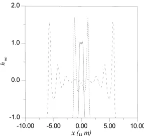
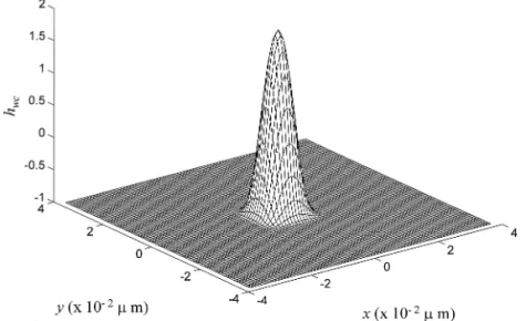
Fig. 13 shows the variation of h_wc for the case of

a square duct with RrL s 0.3. Similar to the case of

Fig. 8, the spatial variation of hwc has a maximum at

a distance about R from the wall, and decreases oscillatory with the distance away from the wall. This implies that a layer of colloidal particles is

Fig. 12. Variation of hwc as a function of r at various radius of cylindrical pore. — — —: 2 R r Ds 0.1; - - -: 2 R r Ds 0.3;

Ž .

: 2 R r Ds 0.5. ucc is calculated by Eq. 24 , and uwc

Ž .

(10)

Fig. 13. Variation of h as a function of x and y for a square duct with RrL s 0.3 and r s 6 = 1023_no.rm3_{. Key: same as Fig. 4.}

wc `

formed near the wall. The qualitative behavior of the spatial variation of the concentration of colloidal particles predicted by the present study is consistent

w x

with that observed experimentally 1 . The maximum and the oscillatory behavior of the spatial variation

of hwc disappear, however, if the bulk particle

con-centration r` is low, as can be seen from Fig. 14.

This is because that as r` decreases, the available

space for particles increases. The average particle concentration for RrL s 0.1, 0.3, and 0.5, are,

re-spectively, 6.15 = 1023_{, 6.37 = 10}23_{, and 6.74 = 10}23

no.rm3 under the conditions of Fig. 4.

In summary, the hypernetted chain approximation is applied to evaluate the direct correlation functions of particle–particle and particle–object interactions. These functions are readily applicable to the determi-nation of the spatial distribution of colloidal particles in the presence of an energy filed. Since the direct correlation functions are described by two indepen-dent equations, the present analysis is also applicable

Fig. 14. Variation of h as a function of x and y for a square duct with RrL s 0.3, and r s 2 = 1023_no.rm3_{. Key: same as Fig. 4.}

(11)

if the hypernetted chain approximation for the direct correlation function of particle–particle interaction is

w x

replaced by the mean spherical approximation 2–4 , andror that for the direct correlation function of particle–wall interaction replaced by the Percus– Yevick approximation. Although only three special cases are examined in the numerical simulation, i.e., planar slit, cylindrical pore, and square duct, the present method can be extended directly to an arbi-trary two-dimensional problem.

Acknowledgements

This work is supported by the National Science Council of the Republic of China.

References

w x1 D.H. Van Winkle, C.A. Murray, J. Chem. Phys. 89 1988Ž .

3885.

w x_{2 P. Gonzalez-Mozuelos, J. Alejandre, M. Medina-Noyola, J.}

Ž .

Chem. Phys. 95 1991 8337.

w x_{3 P. Gonzalez-Mozuelos, J. Alejandre, M. Medina-Noyola, J.}

Ž .

Chem. Phys. 97 1991 8712.

w x4 P. Gonzalez-Mozuelos, J. Chem. Phys. 98 1993 5747.Ž . w x5 J.Y. Walz, A. Sharma, J. Colloid Interface Sci. 168 1994Ž .

485.

w x6 J.Y. Walz, J. Colloid Interface Sci. 178 1996 505.Ž . w x7 R.I. Feigin, D.H. Napper, J. Colloid Interface Sci. 75 1980Ž .

525.

w x8 X.L. Chu, A.D. Nikolov, D.T. Wasan, Langmuir 12 1996Ž .

5004.

w x_{9 J.L. Anderson, J.H. Brannon, J. Polym. Sci., Polym. Phys.}

Ž .

Ed. 19 1981 405.

w10 E.D. Glandt, J. Colloid Interface Sci. 77 1980 513.x Ž . w_{11 N. Ise, T. Okubo, M. Sugimura, K. Ito, H.J. Bolte, J. Chem.}x

Ž .

Phys. 78 1982 536.

w12 K. Ito, H. Nakamura, N. Ise, J. Chem. Phys. 85 1986 6236.x Ž . w13 X. Chu, D.T. Wasan, J. Colloid Interface Sci. 184 1996x Ž .

268.

w14 D.C. Carley, F. Lado, Phys. Rev. 137 1965 A42.x Ž . w15 M. Lozada-Cassou, J. Phys. Chem. 87 1983 3729.x Ž . w_{16 R.J. Hunter, Foundations of Colloid Science, vols. 1 and 2,}x

Oxford University Press, London, 1989.

w_{17 P. Zaini, H. Modarress, G.A. Mansoori, J. Chem. Phys. 104}x Ž1996 3832..

w_{18 L. Yeomans, S.E. Feller, E. Sanchez, M. Lozade-Cassou, J.}x

Ž .

Chem. Phys. 98 1993 1436.

w19 J.A. Greathouse, D.A. McQuarrie, J. Phys. Chem. 100 1996x Ž .

1847.

w_{20 J.A. Greathouse, D.A. McQuarrie, J. Colloid Interface Sci.}x

Ž .

100 1996 1847.

w21 G.N. Patey, J. Chem. Phys. 72 1980 5763.x Ž . w22 M. Lozada-Cassou, J. Chem. Phys. 80 1984 3344.x Ž . w_{23 M. Lozada-Cassou, E. Diaz-Herrera, J. Chem. Phys. 93}x

Ž1990 1386..

w_{24 M. Lozada-Cassou, E. Diaz-Herrera, J. Chem. Phys. 93}x Ž1990 1194..

w_{25 D.A. McQuarrie, Statistical Mechanics, Harper and Row,}x

New York, 1976.

w_{26 A.A. Broyles, S.U. Chung, H.L. Sahlin, J. Chem. Phys. 37}x Ž1962 2462..

w_{27 K.H. Huebner, The Finite Element Method for Engineers,}x

Wiley, New York, 1982.

w28 S.L. Carnie, D.Y.C. Chan, J.S. Gunning, Langmuir 10 1994x Ž .