無線感測網路探勘物體移動路徑機制

全文

(1)國立交通大學資訊工程學系碩士論文. 無線感測網路探勘物體移動路徑機制 On Mining Moving Patterns for Object Tracking Sensor Networks. 研究生：柯郁任指導教授：彭文志. 教授. 中華民國九十四年十月.

(2) 無線感測網路探勘物體移動路徑機制 On Mining Moving Patterns for Object Tracking Sensor Networks. 研究生：柯郁任. Student：Yu-Jen Ko. 指導教授：彭文志. Advisor：Wen-Chih Peng. 國立交通大學資訊工程學系碩士論文. A Thesis Submitted to Department of Computer Science College of Electrical Engineering and Computer Science National Chiao Tung University in partial Fulfillment of the Requirements for the Degree of Master in Computer Science Oct 2005 Hsinchu, Taiwan, Republic of China. 中華民國九十四年十月.

(3) 摘. 要. 由於無線傳輸和嵌入式技術的快速發展，越來越多應用能夠用於無線感測網路，物體移動追蹤乃是前景看好的應用之一。基於物體移動通常具有其規律性，我們提出一追蹤模式，稱為 HTM，以利有效率地探勘物體移動樣式和監控物體。另一方面，由於物體移動通常和其之前所走過的路徑有關，我們採用 variable memory Markov 的方式來探勘物體移動樣式。再者，由於 HTM 有階層的特性，我們利用此特性使移動樣式具有不同解析度。按照探勘出的移動樣式，我們所提出的 HTM 追蹤模式可以精確地預測物體移動路徑，進而降低感測器的能量損耗。更明確的說，HTM 分為兩個階段：資料收集和探勘階段和預測階段。在資料收集和探勘階段中，感測器必須持續感測其所負責的區域以收集物體移動的資料。當資料收集足夠且已探勘出足夠的移動樣式，便進入預測階段。在預測階段中，感測器轉為休眠狀態，只有些許必要的感測器會被喚醒以追蹤物體，藉此達到省電的目的。除此之外，由於感測器的容量有限，我們提出兩個方式來建立 HTM 及一記憶體管理的方法。實驗當果証明我們提出的 HTM 能夠有效地探勘物體移動樣式及追蹤物體。關鍵字：物體追蹤，資料探勘，可變式馬可夫模型.

(4) Abstract The rapid progress of wireless communication and embedded technologies has made wireless sensor networks possible. Since sensor networks are typically used to monitor the environment, one promising application of sensor networks is object tracking. Based on the fact that the movements of the tracked objects generally reflect periodic behaviors, we propose a heterogeneous tracking model, referred to as HTM, to efficiently mine object moving patterns and track objects. Specifically, since the movements of objects have the feature of dependencies, we explore variable memory Markov to mine object moving patterns. Furthermore, due to the hierarchical feature of HTM, multi-resolution object moving patterns are provided. In light of object moving patterns, our proposed HTM is able to accurately predict the movements of objects and thus reduces the energy consumption for object tracking. Explicitly, HTM consists two phases: data collection and mining phase and prediction phase. In data collection and mining phase, all sensors will turn on and monitor the whole sensing region to collect movements of objects. Once collecting sufficient movements of objects, sensor nodes will be in prediction phase. In prediction phases, sensor nodes turn to sleep modes so as to save energy consumption. Only selected sensor nodes will be activated to track objects according to the object moving patterns. Moreover, due to the storage constraint on sensor nodes, we devise two storage strategies to build HTM. Performance of the proposed HTM is analyzed and sensitivity analysis on several design parameters is conducted. Simulation results show that HTM is able to not only effectively mine object moving patterns but also efficiently track objects. Keywords —Object Tracking, data mining, variable memory Markov.

(5) 誌. 謝. 首先我要感謝我的指導教授彭文志老師。兩年來不斷地督促我，不論是研究和做人處事的態度我都學到許多。感謝老師給予我許多寶貴的意見和想法，對我的研究有相當大的幫助。在這兩年內，也讓我在資料探勘這個領域學了不少。另外我要感謝所有實驗室的伙伴們，讓我度過兩年快樂難忘的時光。感謝洪智傑同學和張舜理學長，當我在研究上遇到瓶頸和困難時，總是能夠給予我幫助。感謝李志劭學弟，讓我能夠不需要煩惱生活上的問題。還有原本的大學同學們，雖然不在同一個實驗室，但大家互相加油打氣，給我很大的動力。最後我要謝謝我的家人，不斷地給我鼓勵和支持，讓我能夠打起精神奮鬥下去。謝謝所有關心我的親朋好友們，有了你們，才有這篇論文。謹以此篇論文，獻給各位。.

(6) Contents 1 Introduction. 1. 2 Preliminary. 5. 3 Exploring Moving Patterns for Object Tracking Sensor Networks. 10. 3.1 Overview of Heterogeneous Tracking Model . . . . . . . . . . . . . . . . . . . .. 10. 3.2 Data Collection and Mining Phase . . . . . . . . . . . . . . . . . . . . . . . .. 12. 3.3 Prediction Phase . . . . . . . . . . . . . . . . . . . . . . . . . . . . . . . . . .. 14. 3.4 Recovery Procedure . . . . . . . . . . . . . . . . . . . . . . . . . . . . . . . . .. 16. 3.5 Storage Management . . . . . . . . . . . . . . . . . . . . . . . . . . . . . . . .. 17. 4 Performance Study. 25. 4.1 Simulation Model . . . . . . . . . . . . . . . . . . . . . . . . . . . . . . . . . .. 25. 4.2 Experiments of PES and HTM . . . . . . . . . . . . . . . . . . . . . . . . . . .. 26. 4.3 Sensitivity Analysis of HTM . . . . . . . . . . . . . . . . . . . . . . . . . . . .. 28. 5 Conclusions. 33.

(7) List of Figures 1. An example of showing the advantage of object moving patterns . . . . . . . .. 3. 2. Architecture of Heterogeneous Tracking Model (HTM) . . . . . . . . . . . . .. 5. 3. An illustrative example for moving record collection. . . . . . . . . . . . . . .. 6. 4. The emission tree of the object after the cluster head receives the 17th record, C.. 8. 5. The emission tree with some selected tables after receiving the the 37th record.. 8. 6. An example of prediction and compliance verification . . . . . . . . . . . . . .. 9. 7. A diagram of the heterogeneous tracking model. . . . . . . . . . . . . . . . . .. 11. 8. An illustrative diagram represents the manner of sampling and reporting for low-end sensor nodes in DCM phase . . . . . . . . . . . . . . . . . . . . . . . .. 12. 9. An example of data collection and mining phase . . . . . . . . . . . . . . . . .. 14. 10. An illustrative diagram which shows the behavior of each low-end sensor node in prediction phase . . . . . . . . . . . . . . . . . . . . . . . . . . . . . . . . .. 15. 11. An example of an emission tree traversing for prediction. . . . . . . . . . . . .. 16. 12. An illustrative example of recovery procedure . . . . . . . . . . . . . . . . . .. 18. 13. An illustrative example for the storage strategy 1. . . . . . . . . . . . . . . . .. 21. 14. An illustrative example for the storage strategy 2. . . . . . . . . . . . . . . . .. 21. 15. An illstrative diagram of pruning node in a level i cluster head when its memory space is full and the new node is decided to be inserted. . . . . . . . . . . . . .. 22. 16. An example of profit maintaining for leaf nodes . . . . . . . . . . . . . . . . .. 23. 17. An example of the maintenance of LNode. . . . . . . . . . . . . . . . . . . . .. 25. 18. The object missing rates of PES and HTM . . . . . . . . . . . . . . . . . . . .. 27. 19. The average number of nodes waked up in the recovery procedure . . . . . . .. 27. 20. The missing rates of the storage strategies . . . . . . . . . . . . . . . . . . . .. 28. 21. The level 1 emission tree nodes in the level 2 CH . . . . . . . . . . . . . . . .. 29.

(8) 22. The impact of locality parameter on the prediction hit rate . . . . . . . . . . .. 29. 23. The impact of α for emission tree node maturity verification . . . . . . . . . .. 30. 24. The impact of β for emission tree node maturity verification . . . . . . . . . .. 31. 25. The impact of the probability threshold for prediction . . . . . . . . . . . . . .. 31. 26. The experimental result of phase verification strategy1 . . . . . . . . . . . . .. 32. 27. The experimental results of phase verification strategy2 . . . . . . . . . . . . .. 32.

(9) 1. Introduction. Recent advances in wireless and embedded technologies usher in a new era for our lives. It is expected that an increasing number of small and inexpensive wireless devices (referred to as sensor nodes) are deployed for monitoring various measurements such as temperature, pressure and movements. Applications of wireless sensor networks span a large variety of domains from ecological monitoring to military environments. Due to the nature of wireless sensor networks, sensors have several resource limitations such as power consumption, limited computing capability, smaller storage space and low bandwidth in communications. These limitations of wireless sensor networks have lead to the challenges and issues to the design of sensor networks [1][3][4][8][10]. Since sensor networks are typically used to monitor the environment, one promising application of sensor networks is object tracking. Object tracking sensor networks consist of detecting and monitoring locations of moving objects. It is believed that an object tracking sensor network (abbreviated as OTSN) is viewed as one of the killer applications [2][5][6][11][12][14][15]. An object tracking sensor network is designed for tracking objects with their corresponding unique identifications. In object tracking sensor networks, a number of sensor nodes are deployed over a monitor region. Assume that sensor nodes in the OTSN are static and one sink is required to be the interface for issuing queries and collecting the location of objects. Sensor nodes sense objects with a given sampling frequency to obtain the up-to-date location of objects. Data is reported to the sink according to a report frequency required. Data are sent to the sink via multi-hop communications among sensor nodes. Note that sensor nodes use small batteries for their operations without directly connecting to any power source. As a result, an important design issue in object tracking sensor networks is to conserve the energy as much as possible. Object tracking sensor networks can be roughly categorized into two categories. In the. 1.

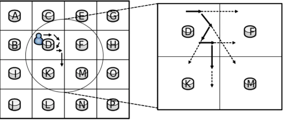
(10) first category, sensor nodes in the OTSN are always active. For example, dynamic convoy treebased collaboration approach is proposed that sensor nodes collaborate to achieve the goal of tracking mobile objects [14][15]. This kind of OTSN can capture the exact location of moving objects. However, since sensor nodes in the network are active all the time, a huge amount of energy consumption is expected. In the second category, only those sensor nodes whose sensing regions are likely to contain tracking objects are active, whereas the rest of sensor nodes are in sleep mode. In previous work [11][12], a sensor node that currently detects objects is called the current node. The current node will predict the location of a moving object and wakes up the sensor nodes (referred to as destination nodes) whose sensing regions are possible contain the objects. If one destination node detects objects successfully, this destination node will become the new current node and will be used to predict the next destination nodes to track objects. If no destination nodes detect the object, flooding recovery will be exploited to find out this missing object. Thus, the performance of a prediction-based object tracking sensor network counts on the prediction accuracy. The authors in [11][12] assume that object movements will remain constant for a period of time. With this assumption, three prediction strategies based on the moving directions and velocities of objects are proposed. In order to ensure the freshness and correctness of moving properties of objects, increasing the sampling frequency in object tracking sensor networks is necessary, incurring more energy consumption when the sampling frequency is increased. Moreover, the object moving history must be passed among sensor nodes for prediction, which incurs extra communication overhead. Notice that when the prediction is not accurate, the worst case is that the flooding recovery will wake all the sensor nodes. In other words, the recovery is unbounded. In reality, objects usually have moving patterns or periodic behaviors [9]. For example, animals are usually have their territories and moving behavior. Consider an example in Figure 1, where the bold arrows are the usual object movement and the dotted arrows are the predicated locations made by sensor D according to the speed and the direction of the object. It can be seen that the 2.

(11) A. C. E. G. B. D. F. H. I. K. M. O. J. L. N. D. F. K. M. P. Figure 1: An example of showing the advantage of object moving patterns object moving direction changes many times. If the sampling frequency is not enough, sensor D is likely to collect wrong information of the object movement and thus makes incorrect predictions. As shown in Figure 1, if sensor D only samples once, the probability of incorrect predictions is 35 . Furthermore, if the sampling frequency are not adjusted dynamically, sensor D may never learn that the object often moves to sensor K and always makes incorrect predictions. To increase the accuracy for prediction-based object tracking sensor networks, mining moving patterns of objects is very important in that the destination nodes are precisely determined from the moving patterns of objects. Clearly, mining moving patterns requires to record each movement of objects for moving log generation, which is unavoidably lead to the energy consumption in object tracking sensor networks. Though improving the accuracy of prediction, utilizing data mining increases the cost of energy consumption. Consequently, we shall explore in this paper an efficient mechanism of mining object moving patterns in a object tracking sensor networks. Our goal is to propose an efficient mining mechanism for mining object moving patterns in object tracking sensor networks and utilize object moving patterns for prediction-based object tracking sensor networks. To facilitate collaborative data collection processing in object tracking sensor networks, the cluster architecture is usually used in which sensors are organized into clusters, with each cluster consisting of a cluster head and sensors. Similar to [1], we propose a heterogeneous tracking model (referred to as HTM), in which a large number of 3.

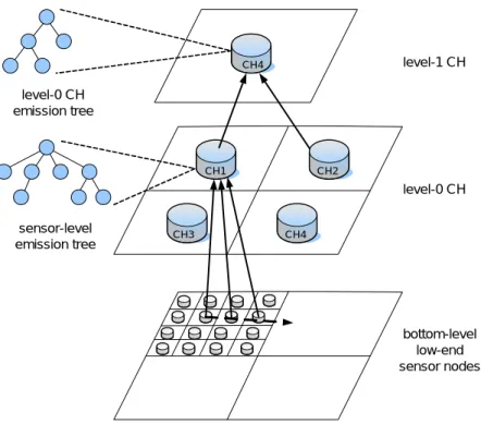
(12) inexpensive sensor nodes perform sense operations and a limited number of powerful sensor nodes (standing for cluster heads) offer data collection, queries and mining capabilities. Figure 2 shows the proposed heterogeneous tracking model, where low-end sensors will sent their sensing data to the corresponding cluster heads and cluster heads have the responsibility for collecting the local moving log of objects from sensor nodes and mining local moving patterns of each object. Notice that cluster heads are powerful sensor nodes with farther communication range, stronger computing power and larger storage space and much more energy than lowend sensors. For the scalability purpose, the cluster heads form a hierarchical architecture for efficiently mining and queries. For simplicity, four neighboring level (i-1) clusters form a larger level i cluster. The level i cluster head is chosen among the four level (i-1) cluster heads. Level i cluster heads will receive the moving records from level (i-1) cluster heads if a object is crossing the boundaries of level (i-1) clusters heads. Thus, level i cluster heads will have the moving behaviors of objects in terms of level (i-1) cluster heads. It is worth mentioning that a multi-resolution data collection mechanism is proposed in our HTM model, where the higher levels of cluster heads will contain coarse object moving patterns and the lower levels of cluster heads will have more precise object moving patterns. In light of object moving patterns, the cluster heads predict the object movements. If the prediction is failure, the recovery procedure will be executed by waking up sensor nodes within the coverage region of the cluster head, showing that a bound number of sensor nodes will be participated in the recovery procedure. There are, however, several issues which we have to address to realize the concept of a heterogeneous tracking model. Specifically, since data collected from low-end sensors can be regarded as data stream, an appropriate mining approach is necessary. Intuitively, the movement of an object is usually dependent on its previous locations. As a result, we will explore the variable memory Markov (termed as VMM) model in which by exploring the dependences of states, VMM is very suitable to capture patterns with high dependences. 4.

(13) Hierarchical Level 1. Hierarchical Level 0. Sensor Level. Figure 2: Architecture of Heterogeneous Tracking Model (HTM) Although the cluster heads are more powerful than low-end sensors, these sensor nodes are still storage constrained. Note that multiple objects are tracked at the same time and thus there will be multiple moving records occupied in constraint storage spaces of cluster heads. Therefore, without reducing the prediction accuracy of cluster heads, two storage strategies for our proposal heterogeneous tracking model are developed in this paper. The rest of the paper is organized as follows. Preliminary is described in Section 2. The detailed object tracking mechanism is presented in Section 3. Performance study is conducted in Section 4. This paper concludes with Section 5.. 2. Preliminary. In this paper, assume that all nodes (i.e., low-end sensor nodes and cluster heads) have their unique identifications and these sensor nodes are well time-synchronized. Suppose that each low-end sensor node is a logical representation of a set of sensor nodes which collaboratively detect an object. When a low-end sensor detects an object, this sensor node will inform the corresponding cluster head of the detected object identification, object arrival time and its sensor identification. It can be seen that the location of an object is represented as sensor 5.

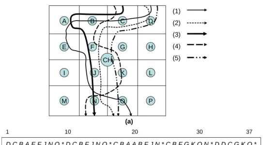
(14) (1) A. B. C. D. (2) (3). E. F. G. H. (4) (5). CH I. J. K. L. M. N. O. P. (a) 1. 10. 20. 30. 37. DCBAEFJNO*DCBFJNO*CBAABFJN*CBFGKON*DDCGKO* (b). Figure 3: An illustrative example for moving record collection. identifications and the moving log of an object is viewed as a moving stream, which is composed of a series of symbols (i.e., sensor identifications). Consider an illustrative example in Figure 3(a), where there are 16 sensor nodes deployed in the coverage region of one cluster head and the object has 5 moving paths. It can be verified that the moving log collected by the cluster head is in a data stream manner shown in Figure 3(b). The symbol "*" means that there is no sensor node reporting the detection of this object (i.e., the object moves out the region monitored by the cluster head and thus the cluster head will not receive any detection message from low-level sensors). Note that cluster heads also have the storage constraint and there are possibly many object moving into the monitoring region of one cluster head. It is impossible to store whole moving records for all objects in cluster heads and let alone scanning moving records multiple times for mining object moving patterns. Therefore, in this paper, we shall address the problem of mining moving patterns with one data scan. Consequently, the variable memory Markov (VMM) model is very appropriate for discovering object moving behavior in that only one data scan is needed for training the VMM model and the movement of an object is in general dependent on its previous locations, satisfying the feature of VMM. As pointed before, the moving records are a series of symbols in a finite alphabet and can 6.

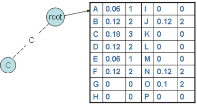
(15) be viewed as the output of a stationary stochastic process. Due to the storage constraint in cluster head and the very nature of moving, i.e., the consecutive moving is dependent on the current location, mining object moving patterns can be regarded as the VMM model training. We borrow a variation of a suffix tree called emission tree from [13] to maintain each VMM model and a buffer in a cluster head is used to hold the most recently records of the stream. An edge in an emission tree represents one symbol which is a sensor identification in moving streams and an emission tree contains tree nodes with the labels defined as the paths from the tree nodes to the root. For example, a tree node labeled as r k ...r 2 r 1 can be reached from the traversal path from root → r 1 → r 2 → ... → r k . Each tree node maintains the appearing counts and the conditional probabilities of all possible next nodes with this node labeled as a prefix. Assume that the moving records held by the buffer are r 1 ...r l−1 and initially, the emission tree has only one root node with the counts of each symbols appearing in the buffer so far. If the count of the symbol r i is larger than the threshold, minimal support, one child node labeled as r i will be inserted into the emission tree. With an example profile given in Figure 3(b) and the minimal support being 3, the cluster head receives the 17th record (i.e., C in this example). Figure 4 shows the configuration of the emission tree so far. It can be seen that the root node maintains the conditional probabilities and the counts of sensors and since the count of C is larger than the minimal support (i.e., 3), one child node labeled as node C is included in the emission tree. Assume that the moving records held by the buffer are r 1 ...r l−1 and when a new record, r l , arrives into the buffer, those statistic information (i.e., counts and the probabilities) should be updated accordingly. If the node r l−j ...r l−2 r l−1 is the furthest node we can reach from the root of the emission tree along the path root → r l−1 → r l−2 → ... → r 1 , for each node r l−k ...r l−2 r l−1 , the count N(rl−k ...rl−1 rl ) should be increased by 1 and the conditional probabilities P (rl |rl−k ...rl−2 rl−1 ) and P (x|rl−k ...rl−2 rl−1 , x 6= rl ) must be adjusted. Once the updates of these tree nodes are performed, if N(rl−k ...rl−1 rl ) is larger than the minimal support, rl−k ...rl−1 rl becomes a frequent subsequence and thus a new node 7.

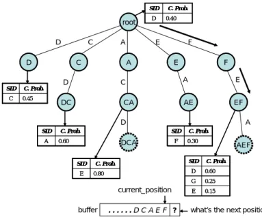
(16) Figure 4: The emission tree of the object after the cluster head receives the 17th record, C.. Figure 5: The emission tree with some selected tables after receiving the the 37th record. labeled as rl−k ...rl−1 rl will be inserted as a child node of node rl−k+1 ...rl−1 rl . Figure 5 shows the tree after all the 37 records are processed by the cluster head. In order not to distract users from the main theme of this paper, interested readers are referred to [13] for the detailed procedure of constructing an emission tree. VMM model is trained on the fly and not all the tree nodes are stable for predicting. Consequently, there are two nodes in an emission tree: one is the mature node and the other is immature node. Mature nodes are those tree nodes in which a certain amount of records are collected and the conditional probabilities are stable. When predicting the next movement, only mature node is participated in prediction. Consider an example in Figure 6. Only a portion of information is shown in the figure. The nodes with bold sideline are mature nodes and the nodes with dotted sideline are immature nodes. Suppose that the most recent records held in the buffer are D, C, A, E, F in the chronological order. If we want to predict the next symbol with these records as prefix, we traverse the tree along the path root → F → E → ... 8.

(17) SID D. root D. C. D. A. C. C. E. F. A. D SID. C. Prob. 0.40. E. C. F A. E. AE. EF. C. Prob. 0.45. DC. CA D. SID A. A. C. Prob.. SID. 0.60. DCA SID E. F. 0.30. SID. C. Prob. 0.80. current_position buffer. C. Prob.. ......DCAEF ?. AEF C. Prob.. D. 0.60. G. 0.25. E. 0.15. what’s the next position ?. Figure 6: An example of prediction and compliance verification → D. Since node AEF is immature, the traversing terminates at node EF. The probability distribution in the table of node EF shows that D has the highest conditional probability 0.60 to be the next symbol. To justify whether a node is mature or not, we explore L∞ distance, which is defined as follows: Definition 1: For a node y with the corresponding probability table denoted as x and the 0. 0. 0. number of tuples in table x is n, L∞ (x, x0 ) = max(|dx1 − dx1 |, |dx2 − dx2 |, ... |dxn − dxn |), where dxi represents the probability value for tuple i in table x and table x0 is the probability table after updating. In light of Definition 1, for node y, if L∞ (x, x0 ) ≤ α for β times of successive updates, node y becomes a mature node, where α and β are given by users and will be application dependent parameters.. 9.

(18) 3. Exploring Moving Patterns for Object Tracking Sensor Networks. Based on the mining object moving patterns, we propose a heterogeneous tracking model (referred to as HTM) for object tracking sensor networks. In Section 3.1, the overview of HTM, which is composed of two phases (i.e., data collection and mining phase and prediction phase) is described. Specifically, with moving records generated in HTM, we devise an efficient mechanism for data collection and mining in Section 3.2. In Section 3.3, once mining object moving patterns, sensor nodes will be in prediction phase so as to save as much energy as possible. A recovery procedure is developed in Section 3.4. In Section 3.5, two storage strategies are devised.. 3.1. Overview of Heterogeneous Tracking Model. Our proposed heterogeneous tracking model consists two phases for each cluster heads which is shown in Figure 7. In data collection and mining phase, all sensors will turn on and monitor the whole sensing region to collect moving records of objects. Once an object is detected by a sensor node, the sensor node will inform its corresponding cluster head by generating one moving record. At the same time, the mining procedure (i.e. the VMM model training for each object) is performed in the cluster head. Furthermore, similar to the concept of message pruning trees [6], when one object crosses the boundary of two neighboring cluster heads, these two cluster heads will transmit location updated messages upward the hierarchical tracking model until their common parent node receives the messages. Then the nodes along the message forwarding path will also have these location updated messages used to train VMM models in higher level cluster heads. Note that if an object Obj i is in the coverage of cluster head CH j , CH j will predict the movement of Obj i and justify the correctness of the prediction. To decide whether a cluster head can transit to the prediction phase or not, we define two 10.

(19) Data Collection and Mining Phase. hit_rate >= threshold1 and hit number >= threshold2. Prediction Phase. wrong. Recovery Procedure. hit_rate < threshold. Figure 7: A diagram of the heterogeneous tracking model. threshold values to verify. If the average prediction hit rate ≥ δ and the average number of correct predictions ≥ σ, the cluster head will be in the prediction phase. The performance study of these two threshold values (i.e., δ and σ) will be conducted in our experiments. If the cluster head is in the prediction phase, sensor nodes within the coverage of this cluster head will turn into sleep modes. The cluster head in the prediction phase will estimate the possible locations of an object and wake up those sensor nodes whose sensing ranges are able to sense the object. If the cluster head accurately predict the location of the object, the sensor nodes capturing the object will notify the cluster head. Intuitively, this operation is similar to the feedback of the prediction, which can be viewed as data collection as well. It is possible that the prediction is not correct and thus sensor nodes cannot sense the object. In this case, the recovery procedure will be executed in the cluster head. The cluster head will wake up more sensor nodes to sense the missing object. Once sensing the missing object, sensor nodes will sends a location message to the cluster head. This location message will be used to train VMM model so as to increase the prediction accuracy. From these feedback messages, VMM mining models will be trained and is able to generate object moving patterns. In light of these moving patterns mined, the prediction-based heterogeneous tracking model is able to save more energy.. 11.

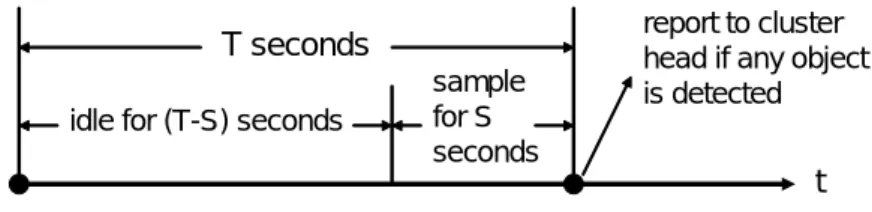
(20) T seconds idle for (T-S) seconds. sample for S seconds. report to cluster head if any object is detected. t. Figure 8: An illustrative diagram represents the manner of sampling and reporting for low-end sensor nodes in DCM phase. 3.2. Data Collection and Mining Phase. In this phase, moving records of objects (referred as logs) will be collected for mining object moving patterns. In the beginning, since there are no moving records available, sensor nodes and cluster heads turn on their power and radio to monitor objects. Given a sampling frequency, the low-end sensors sense and report the sensing information to the sink every T seconds. Similar to the work in [12], each low-end sensor node keeps idle for (T - S ) seconds, and then senses the environment for S seconds. When a low-end sensor detects a moving object, this sensor node will send one message containing the time and the object sensed to the cluster head in charge of this sensor node. After receiving the detection message, the cluster head will have a moving record represented as (i, j, t) meaning that sensor i detects object j at time t. As mentioned before, in our proposed tracking model, the cluster heads form a hierarchical architecture for efficient mining and queries. For simplicity, four neighboring level (i-1) clusters form a larger level i cluster. The level i cluster head is chosen among the four level (i-1) cluster heads. Level i cluster heads will receive the moving records from level (i-1) cluster heads if an object is crossing the boundaries of level (i-1) clusters heads. In order to reduce the amount of location updates among cluster heads, we employ the message pruning concept [6][7]. The goal of a message pruning concept is to reduce the number of location update messages for object tracking. By exploring the concept of message pruning, if one object crosses the boundary of two neighboring cluster heads, these two cluster heads will transmit location update messages upward the hierarchy until their common parent receives. 12.

(21) the messages. As such, the cluster heads along the message forwarding path should generate the higher level moving records that indicates which cluster head and the object detected by their low-end sensors. Once having higher level moving records, cluster heads at higher levels are able to mine more coarse object moving patterns. Given moving records of objects, each cluster head will exploit the VMM model for mining object moving patterns. Note that without collecting moving records in the sink, our proposal heterogeneous tracking model is able to achieve in-network mining in that mining object moving patterns is performed while moving records are forwarded in the sink. Furthermore, cluster heads at higher levels have coarse object moving patterns, whereas cluster heads at lower levels contain finer object moving patterns. Note that if an object Obj i is in the coverage of cluster head CH j , CH j will predict the movement of Obj i and justify the correctness of the prediction. To decide whether a cluster head can transit to the prediction phase or not, we define two threshold values to verify. If the average prediction hit rate ≥ δ and the average number of correct predictions ≥ σ, the cluster head will be in the prediction phase. The performance study of these two threshold values (i.e., δ and σ) will be conducted in our experiments. Consider an example in Figure 9, where the dash line represents the moving path of the object Obj 1 and CH 4 is the level 1 cluster head chosen from the 4 cluster heads in level 0. The low-end sensors along the moving path in the territory of cluster CH 1 will detect Obj 1 and notify CH 1 in the chronological order. Then CH 1 uses these records to update the emission tree of Obj 1 . When Obj 1 departs from CH 1 and moves into CH 2 , CH 1 will not receive any detection messages from low-end sensors and assumes that Obj 1 is out of its territory. If cluster heads cannot receive any detection message, ’*’ will be appended to the tail of the buffer. As such, CH 1 will append a ’*’ symbol to the tail of the Obj 1 ’s sensor-level buffer. As can be seen in Figure 9, this object moves to the coverage of CH 2 and one of its sensor nodes reports the location of this object. According to the message pruning concept, CH 1 sends a departure message, whereas CH 2 will send an arrival message upward the hierarchy. Since 13.

(22) level-1 CH. CH4. level-0 CH emission tree. CH1. CH2. level-0 CH sensor-level emission tree. CH4. CH3. bottom-level low-end sensor nodes. Figure 9: An example of data collection and mining phase CH 4 is the common parent node of CH 1 and CH 2 . Thus, the location update message will not be forwarded to upper levels. In addition, CH 4 will append ’CH 2 ’ to the tail in the moving records for Obj 1 . With the movements of Obj 1 , the moving records are generated accordingly and object moving patterns are mined via the emission tree construction. Note that since the object movements usually exhibit locality, the incoming rates of moving records of upper level cluster heads is slower than those of lower level cluster heads. In order to speed up the training of upper level emission trees, we have to specify smaller min_sup and the number of times β for verifying node maturity.. 3.3. Prediction Phase. When a cluster head is in this phase, the cluster head will allow the low-end sensor nodes to be in sleep modes. If an object Obj i is within the coverage region of level 0 cluster CH j , CH j is in charge of predicting the next movement of Obj i . By traveling the emission tree of Obj i ,CH j will wake up those sensor nodes appearing in the emission tree with their probabilities ≥. 14.

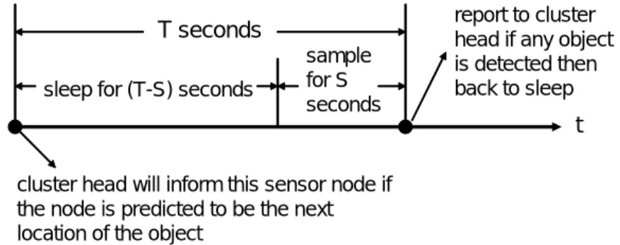
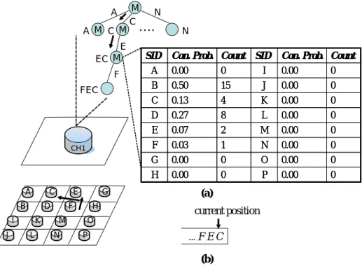
(23) T seconds sleep for (T-S) seconds. sample for S seconds. report to cluster head if any object is detected then back to sleep. t cluster head will inform this sensor node if the node is predicted to be the next location of the object. Figure 10: An illustrative diagram which shows the behavior of each low-end sensor node in prediction phase threshold γ. Assume that the sampling frequency is set to T seconds. As shown in Figure 10, after sleeping for (T - S ) seconds, those sensor nodes determined by CH j will be activated for S seconds. If one of these sensor nodes detects Obj i , this sensor node will send an ACK message to CH j . Since the predicted sensor nodes are able to successfully detect objects, all of these sensor nodes waked up will turn to sleep. According to the response message from low-end sensor nodes, CH j will update the hit rate, the buffer and the emission tree of object Obj i . If the predicted sensor nodes are not able to detect object Obj i , which means that the prediction of the next movement of Obj i is wrong, CH j will initiate the recovery procedure. Note that if the average hit rate for objects becomes smaller than the specified threshold δ, CH j will be in the the data collection and mining phase for training VMM models so as to increase the prediction accuracy. Consider an example in Figure 11, where Figure 11(a) shows the emission tree of Obj i in CH j and Figure 11(b) is the buffer of CH j for Obj i . Given the most recent moving records of the buffer, CH j traverses the emission tree along the path root → node C → node EC → node FEC. Assume that node FEC is not mature yet and the probability threshold for the determination of candidate sensor nodes is 0.5. Thus, the traversing terminates at node EC. The probability table of node EC shows that the sensor node B will be activated since the corresponding probability of node B satisfies the probability threshold (i.e., 0.5). If sensor node B is able to detect Obj i , sensor node B will send an ACK message to CH j 15.

(24) A A M C M E EC M F FEC. CH1. A. C. B I J. E. D K L. N. N. …. SID A. N Con. Prob. Count 0.00. SID. 0. Con. Prob. Count. I. 0.00. 0. B. 0.50. 15. J. 0.00. 0. C. 0.13. 4. K. 0.00. 0. D. 0.27. 8. L. 0.00. 0. E. 0.07. 2. M. 0.00. 0. F. 0.03. 1. N. 0.00. 0. G. 0.00. 0. O. 0.00. 0. H. 0.00. 0. P. 0.00. 0. G. F M. M C. (a). H. current position. O P. ... F E C. (b). Figure 11: An example of an emission tree traversing for prediction. and one moving record (i.e., (sid, Obj i , t)), will be appended to the buffer for next location prediction. On the other hand, if sensor node B cannot detect Obj i , the recovery process has to be started. Moreover, the cluster head appends symbol "*" to the buffer for Obj i . From feedbacks of sensor nodes (i.e., Acknowledge message), though a cluster head is in the prediction phase, these feedbacks are beneficial to train VMM models as well.. 3.4. Recovery Procedure. When cluster head CH j cannot precisely predict the sensor nodes to detect object Obj i , the recovery procedure will be performed to track object Obj i . The possible location of object Obj i can be conducted into two cases. One is that Obj i is still in the coverage region of CH j . The other is that object Obj i moves into the coverage regions of other cluster heads. According to the observations above, cluster head CH j will first check whether Obj i is still in the coverage region of CH j by waking up all sensor nodes under the coverage region of CH j . If one of these sensor nodes captures Obj i , the sensor node still sends an ACK message to. 16.

(25) CH j . Otherwise, CH j informs its higher level cluster head (i.e., the parent node of CH j ) since higher level clusters have coarse moving patterns of Obj i used to predict possible cluster heads of object Obj i . By traveling the emission tree of Obj i and selecting the node with the highest probability, one cluster head, in which object Obj i is likely to appear, will be determined. Then, the selected cluster head will downward to the lowest level cluster heads to estimate the fine moving patterns of object Obj i . If the object is still not found in the selected cluster head, the parent cluster head will select other cluster heads to perform the recovery procedure. If none of these cluster heads finds the missing object, the parent cluster head will forward the upper level cluster head for the recovery purpose. As mentioned before, each level cluster head has different resolution object moving patterns. In light of these multi-resolution object moving patterns, the number of sensor nodes activated for the recovery procedure is bound, showing the advantage of utilizing our proposal heterogeneous tracking model. Consider an example in Figure 12. Since CH 1 misses the object, CH 1 informs its parent CH 5 and appends ’*’ to the tail of buffer in CH 1 . By traversing the emission tree of the object in CH 5 , CH 5 predicts that the object is likely to be in the coverage region of CH 2 and let CH 2 track the missing object. The sensor nodes within the coverage region of CH 2 will be activated to detect the missing object. Once receives the detection message from one of these sensor nodes, CH 2 will update the corresponding emission tree. Note that CH 2 will send a location update message to its parent CH 5 . Accordingly, CH 5 will also appends ’CH 2 ’ to the tail of its buffer and updates the corresponding emission tree.. 3.5. Storage Management. As mentioned above, in our proposed heterogeneous tracking model, those higher levels cluster heads should store moving records of objects. In general, cluster heads are also sensor nodes with more computing power and storage spaces. These cluster heads are intrinsically sensor nodes as well. As such, cluster heads may suffer from the storage saturation problem in which 17.

(26) level 0 buffer. CH5. CH2. 6. append. 1. object miss message. sensor-level buffer *. 5. object found message 3. predict. CH1. CH2. 2. append CH4. CH3. sensor-level buffer * 4. append the sensor_ID of the node which detects the object. Figure 12: An illustrative example of recovery procedure there is no available free storage space for incoming moving records. Consequently, we propose an efficient storage management for cluster heads. Assume that level i cluster head is chosen among level (i - 1) cluster heads. It is possible that a level i cluster head will maintain moving records of all level emission trees for each object. As result, higher level cluster heads will suffer more enormous storage overhead. Let Pi be the probability that an object leaves its current level i cluster and di is the updating cost (i.e., hop counts) from the level i cluster head to the level (i+1) parent node. Furthermore, suppose that there are (k+1) levels in the hierarchical tracking model (i.e., level 0 to level k). Therefore, the expected value of communication cost among cluster heads, denoted as E[C], for one object can be evaluated as following:. E[C] = Pk−1 =. k−1 X. k−1 X i=0 i Y. ((. i=0. j=0. di + (1 − Pk−1 )Pk−2. (1 − Pk−j ))Pk−i−1. k−2 X. i=0 k−i−1 X. di + (1 − Pk−1 )(1 − Pk−2 )Pk−3. k−3 X. di + .... i=0. dl ), where Pk = 0. l=0. Given the leaving probabilities P0 to Pk , it can be seen that the updating costs d0 to dk−1 are the dominated factors for the value of E[C]. The values of di are dependent on the network topology. Therefore, two storage strategies are developed as follows. Consider an example of 18.

(27) the strategy one in Figure 13. Suppose that the sensor field is divided into a 24 × 24 grid and the sink (i.e., the level 4 cluster head) is at the center. Each grid is a level 0 cluster head and the level i cluster head, the nearest to the sink in a 2i+1 × 2i+1 cluster, is selected to be the level (i+1) cluster head. In Figure 13, the number i represents cluster heads of level 0 to level i. The arrows show the transmission for each level i CH sending the location updating messages to its level (i+1) parent. By observation, the expected value E1 [di ] = 2i , where i =[0,2] and E1 [d3 ] = 1. Figure 14 shows the storage strategy two, where the number i means that the grid is a level 0 cluster head and a level i cluster heads. Once a level 0 cluster head is selected to be the upper level cluster head, this cluster head will never be selected again. The hierarchy construction principle is that among the level 0 cluster heads which are not selected yet, the nearest one to the level (i+1) cluster head in each 2i × 2i cluster will be chosen to be the child node of the level (i+1) cluster head. It can be verified that the expected value E2 [di ] is almost the same as E1 [di ]. Let E[S] be the expected value of the storage cost for each cluster head (i.e., average level that a CH is in charge of). Then E1 [S] and E2 [S] can be evaluated as follows: In the strategy one, a level i cluster head must maintain sensor level, level 0, ..., level (i-1) trees (i.e., (i+1) levels totally), then,. (k + 1) + (41 − 40 )k + (42 − 41 )(k − 1) + ... + (4k − 4k−1 ) 4k 4 − 4−k = 3. E1 [S] =. In the strategy two, each cluster head maintains the trees at most 2 levels of information. Then,. 19.

(28) k. 2( 4 3−1 ) + E2 [S] = 4k 4 − 4−k = 3. 2×4k +1 3. After the estimation of the average storage cost, we can evaluate the variance of the storage cost in strategy 1 and 2.. ((k + 1) − E1 [S])2 + 3(k − E1 [S])2 + ... + 3 × 4k−1 (1 − E1 [S])2 k Pk−1 i 4 −k 4−k 1 2 (k + 3 − 3 ) + 3 i=0 (4 ((k − i) + 4 3 − 43 )2 ) = k Pk−1 i 4 1 2 (k − 3 ) + 3 i=0 (4 (k − i − 2)2 ) ≥ 4k 41 2 15 17 5 10 = k − k + 4−k k − 4−k + 12 4 3 9 3. V1 [S] =. k. k. (2 − E2 [S])2 ( 4 3−1 ) + (1 − E2 [S])2 ( 2×43 +1 ) V2 [S] = 4k 2 4−k 4−2k = − − 9 9 9. It can be seen that V1 [S] will be much larger than V2 [S] when k increases. Note that strategy 2 has much better load balance than strategy 1. Load balance is an important issue for the in-network mining and prediction in our work. If a cluster head has to maintain the trees for too many levels, its storage may becomes full soon. Once the storage expires, the trees can not be enhanced anymore and it affects the prediction accuracy directly. In strategy 2, the hot spot problem is solved. In each cluster head, there will be much more memory space for the emission tree training at different levels.. 20.

(29) 1. 1. 1. 1. 1. 1. 1. 1. 1. 2. 1. 2. 2. 1. 2. 1. 1. 1. 1. 1. 1. 1. 1. 1. 1. 2. 1. 3. 4. 1. 2. 1. 1. 2. 1. 3. 3. 1. 2. 1. 1. 1. 1. 1. 1. 1. 1. 1. 1. 2. 1. 2. 2. 1. 2. 1. 1. 1. 1. 1. 1. 1. 1. 1. Figure 13: An illustrative example for the storage strategy 1.. 1. 1. 1. 1. 1. 2. 2. 1. 1. 1. 1. 2. 1. 1 1. 2. 1. 1. 1. 1. 1. 1. 1 1. 2. 1. 2 1. 1. 1. 1. 1. 1. 2. 1. 2 1. 1. 1. 1. 1. 1. 3. 2. 1. 2. 1. 1. 3. 4. 1. 3. 3. 2. 1. 2. 1. 1. 1 1. 1. 2. 1. 1. 1. 1. 1. 1. 1. 2. 1. 1. 2. 2. 1. 1. 1. 1 1. 1. 1 1. 1. 1. 1. Figure 14: An illustrative example for the storage strategy 2.. 21.

(30) level (i - 1) trees. sensor level trees T1. T2. T3. T4. T5. hit_rate > 0.6. hit_rate < 0.6 hit_rate < 0.8. insert. prune. Figure 15: An illstrative diagram of pruning node in a level i cluster head when its memory space is full and the new node is decided to be inserted. Applying the hierarchy construction approach as shown in Figure 14, a level i (i ≥ 1) cluster head only has to maintain two level buffers (i.e., the sensor-level and (i-1)th level)and emission trees for each object. Since there are multiple objects and the storage of each cluster head is limited, it is still possible that the storage requirement exceeds the limit. Hence, a storage management strategy is necessary for dealing with this situation. When the memory space of a cluster head is full and the count of one symbol in the table maintained by an emission tree node becomes ≥ min_sup, we have to decide to prune other nodes so that the newborn node can be inserted into emission trees. We specify a threshold. and if the. prediction hit rate of the tree to which the newborn node belongs is already larger than , we can ignore the insertion since this emission tree already has higher prediction rates. Otherwise, we must select an appropriate node to be pruned from other trees. The pruning mechanism consists two steps:(1). select the tree to be pruned and (2). select the node to be pruned. 1) Select the tree to be pruned. Each object usually has its own moving behavior. An object may stay in some regions more frequently than other regions. Hence, the reporting rates of. 22.

(31) root. A. DA. CDA. B. DB. D. CD. CDB. Figure 16: An example of profit maintaining for leaf nodes objects in each cluster head will be different. For the tree selection, each tree maintains a counter. Once a tree is updated, the counter of the tree is increased by one. In addition, each counter minuses one every T periods. A tree with a lower counter value means that it is not often used than other trees. Note that since object movements usually exhibit locality, upper level trees will be updated infrequently and grow with a slower speed than lower level trees. If we just select the tree with the minimal counter value, the upper level trees will have more chances to be pruned and the emission tree at higher levels of cluster heads will be hard to achieve good accuracy. Hence, we only select the same level tree, to which the newborn node will be inserted. To guarantee that the accuracy of each tree is acceptable, we specify a threshold ε. Suppose that the new node will be inserted into a level i emission tree. Among other level i trees with their prediction hit rates ≥ ε, the tree with the minimal counter value will be selected. Consider an example in Figure 15, where the size of a tree stands for the access counter value of the tree. Let. = 0.8 and ε = 0.6. Since the hit rate of tree T 1 < 0.8,. we decide to insert the new node into T 1 and prune one node in T 2 ~T 5 . Although T 2 has the minimal counter value, its hit rate < 0.6. T 2 will not be selected and T 4 is next selected. Since the hit rate of T 4 > 0.6, T 4 is then selected to be pruned. 2) Select the node which will be replaced by the new node. Once the tree is selected, we must prune the node such that there will be less impact to the selected emission tree. For 23.

(32) the node selection, each tree maintains the profits for each leaf node which no other node is derived from it. Let LNode is the set of all these nodes. Consider an example in Figure 16, assume that node CD, CDA and CDB are leaf nodes. Since node CDA and CDB are derived from node CD, we will not take node CD into consideration. The probability of a node represents the importance of the node to the tree. A lower probability means that the node is accessed infrequently than other nodes. Thus, we take the node probability as one factor for the node profit. In addition, since only the mature nodes will be used for prediction and probability estimation, the mature nodes bring more profits than the immature ones. Among the immature nodes, there are still differences of the mature degree. An immature node, which is likely to be mature, is more important than a whole new node. Thus, we must first check whether a node is mature or not. let N be the number of times that the L∞ distance of the probability distribution of node x. The mature degree of a node x, denoted by MD(x), is defined as follows:. MD(x) =. N β. With the above two factors, the profit function of a node x, expressed by Profit(x), is formulated as follows:. Profit(x) = P (x) × (MD(x) + c), where c is a real constant used as the base The node with the minimal profit value in LNode will be chose to be pruned. To reduce the cost of maintaining LNode, if a node becomes mature, we won’t continue to update the probability entries in the table of the node. Consider an example in Figure 17. The nodes with bold sideline are mature nodes and the nodes with dotted sideline are immature nodes. Node DCAE is a node in LNode. Since node DC and node DCA is immature, P (DCAE) + P (D)×P (C|D)×P (A|C)×P (E|CA). We don’t have to recalculate P (DCAE) 24.

(33) root D D. A. C C. A. CA. DC. DCA. Figure 17: An example of the maintenance of LNode until one of node DC and node DCA becomes mature. With the pruning mechanism, there will not be a specific tree which is always selected to be pruned. Since if the prediction hit rate of a tree becomes < ε, the tree will not be selected anymore. Furthermore, even if the hit rate of a tree becomes lower due to the node pruning, it still has chances that the nodes can be inserted back.. 4. Performance Study. In this section, experimental results are presented. The simulation model is described in Section 4.1. The comparison of our scheme with PES scheme [12] is conducted in Section 4.2. Finally, the sensitivity analysis of in-network mining approach is described in Section 4.3.. 4.1. Simulation Model. There are 3 levels in our proposed heterogeneous tracking model and we deploy 9 low-end sensors in each level 0 cluster. Hence, there are 16 level 0 CHs, 4 level 1 CHs, one level 2 CH, and the number of low-end sensors is 144. To simulate the object movements, we generate VMM model trees for each object in each cluster head. In addition, the city mobility model 25.

(34) [6] is used to simulate object movements with locality. With the model, each object has a probability p 1 to determine whether it should leave its current level 1 cluster, and a probability 1 - p1 to stay. In the former case, it will choose a level 1 cluster as the next position according to its VMM model tree in the level 2 CH (It may stay in the current level 1 cluster). In the latter case, it has a probability p0 to determine whether it should leave its current level 0 cluster, and a probability 1 - p0 to stay. Similarly, in the former case, it will choose a level 0 cluster as the next position according to its VMM model tree in the parent. In the latter case, it will stay in its current level 0 cluster. In all cases above, the VMM model looking up procedure is repeated until the object has decided to move to which low-end sensor monitored i+1. region. The probability pi is determined by an exponential probability pi = e−C·2. , where C. is a positive constant. A higher value of C means higher locality.. 4.2. Experiments of PES and HTM. To conduct the experiments of PES scheme in [12], we simply utilize the object positions at two successive time units to evaluate the object speed and direction. The object missing rates of PES and HTM are shown in Figure 18. Since the sampling frequency is not enough, the evaluated object speed and direction is almost incorrect, PES cannot precisely predict the object movement. It can be seen that with the time advances, the object missing rate of HTM decreases since the moving patterns are extracted gradually. Since the network in PES is homogeneous, we compare the average number of low-end sensors waked up by recovery procedure. PES wakes up much more sensors because the missing rate is high and the recovery scope is unbounded. Due to the feature of hierarchical clustering, the number of sensors activated in the recovery procedure is bounded.. 26.

(35) 1. PES HTM. 0.5. 0 18 00. 0 14 00. 0 10 00. 60 00. 0 20 00. Missing Rate. Missing Rate. Time. Figure 18: The object missing rates of PES and HTM. 150 100 50. HTM. 10 00 0 14 00 0 18 00 0. PES 60 00. 0 20 00. The Number of Nodes. The Number of Sensor Nodes waked up by Recovery. Time. Figure 19: The average number of nodes waked up in the recovery procedure. 27.

(36) 0.7 0.6 Missing Rate. 0.5 0.4. Strategy 1 Strategy 2. 0.3 0.2 0.1 0 1. 3. 5. 7. 9. 11. 13. 15. Number of Objects. Figure 20: The missing rates of the storage strategies. 4.3. Sensitivity Analysis of HTM. First, we investigate the impact of the two storage strategies. We set the value of min_sup to be 15, α to be 0.01, β to be 6, C to be 3, δ to be 0.6, σ to be 10,. to be 0.7, ε to be 0.5. and each CH can store 30 emission tree nodes. Figure 20 shows the object missing rate in the level 0 cluster at which the sink is located. With the clustering strategy 1, the sink node has to maintain the emission tree nodes for 3 levels so the memory space is insufficient for each level and the emission tree growing is limited. Hence, the missing rate increases when the number of objects increases. However, clustering strategy 2 is a load balance clustering approach and the sink will have more sufficient memory space for the emission tree training at different levels. In the next experiment, we let the CH can store 500 emission tree nodes. Figure 21 shows the average number of level 1 emission tree nodes for each object in the sink. It can be seen that clustering strategy 2 is better than clustering strategy 1 since the sink can have more sufficient memory space to store more level 1 emission tree nodes. To observe the impact of locality parameter C on the prediction hit rate of our scheme,. 28.

(37) Average number of Lv1 emission tree nodes in Lv2 CH. 10 8 6. Strategy 1. 4. Strategy 2. 2 0 5. 10. 15. Number of Objects. Prediction Hit Rate. Figure 21: The level 1 emission tree nodes in the level 2 CH. 0.85 0.8 0.75 0.7 0.65 0.6 0.55 0.5 0.45 0.4. α = 0.1 α = 0.05 α = 0.01. 0.5. 1. 1.5. 2. 2.5. 3. 3.5. C. Figure 22: The impact of locality parameter on the prediction hit rate we set min_sup to be 15, β to be 6, δ to be 0.6, σ to be 10,. to be 0.7, ε to be 0.5, each CH. can store 500 emission tree nodes, α to be 0.01, 0.05 and 0.1 respectively. Figure 22 shows the average prediction hit rate in each level 0 cluster. It can be seen that the prediction hit rate tends to increase as the value of C increases. The reason is that if C is high, the object tends to stay in the current cluster so that the CH can get much more moving records for mining more quickly and the CH would seldom make incorrect predictions when the object leaves its current level 0 cluster. Next, we conduct the experiments to see the impact of α on prediction hit rate. We set 29.

(38) Prediction Hit Rate. 0.84 0.82 0.8 MinSup = 15, β= 6 MinSup = 25, β= 6 MinSup = 35, β= 6. 0.78 0.76 0.74 0.72 0.7 0.01. 0.05. 0.1. 0.15. α. Figure 23: The impact of α for emission tree node maturity verification β to be 6, min_sup to be 15, 25, and 35 respectively. The experimental results are shown in Figure 23. It can be seen that the prediction hit rate decreases as the value of α increases. Since a lower α means that a CH needs more moving records to let the probability variation of a tree node between two successive updates ≤ α. And more updates in a node means that the probability distribution in the node is more stable and close to the real probability distribution. To conduct the experiments of another emission tree node maturity verification parameter β, we set α to be 0.01, min_sup to be 15, 25, and 35. Figure 24 shows the experimental results. We can conclude that the value of β should not be too small or too big. If the emission tree training in a CH just gets start, it is possible that the probability difference is very small when the CH receives the same record for a few times. If β is very small, we may make incorrect decision that the node is mature. If β is big, then the appropriate nodes can not be used for prediction as soon as possible. From Figure 23 and Figure 24, it can be seen that the major factor of maturity verification is α. Now, we observe the impact of the probability threshold for prediction on prediction hit rate. Figure 25 shows the experiment results of the average level 0 CH prediction hit rate with various probability threshold. A low threshold means that the CH will predict more sensors. 30.

(39) Prediction Hit Rate. 0.85 MinSup = 15, α= 0.01 MinSup = 25, α= 0.01 MinSup = 35, α= 0.01. 0.8 0.75 0.7 0.65 1 2 3 4 5 6 7 8 9 10 11 12 β. Prediction Hit Rate. Figure 24: The impact of β for emission tree node maturity verification. 0.8 0.7 0.6 0.5 0.4 0.3 0.2 0.1 0. α= 0.01. α= 0.05. α= 0.1. 0.1. 0.2. 0.3. 0.4. 0.5. Probability Threshold. Figure 25: The impact of the probability threshold for prediction as the next position so the prediction hit rate will be higher. A high threshold has low hit rate due to the reason that there may be no sensor with probability which is higher than or equal to the threshold so the CH won’t predict any sensor as the next position. Finally, we conduct the experiments of the phase verification for two strategies. For the experiments, we set δ to be 0.5, 0.6, 0.7, σ to be 10 and the object number to be 7. In strategy1, a CH simply estimates the average hit rate and the average prediction hit numbers of all objects. If the average hit rate ≥ δ and the average hit numbers ≥ σ, then the CH will turn into prediction phase. The experimental results of strategy 1 is shown in Figure 26. It can be. 31.

(40) Number of Lv0 CH in Prediction Phase. 8 7 6 5 4 3 2 1 0. δ= 0.5,σ= 10 δ= 0.6,σ= 10 δ= 0.7,σ= 10. 4000. 8000. 12000 16000 20000 Time. Number of Lv0 CH in Prediction Phase. Figure 26: The experimental result of phase verification strategy1. 20 15. δ= 0.5,σ= 10 δ= 0.6,σ= 10. 10. δ= 0.7,σ= 10 δ= 0.8,σ= 10. 5 0 100. 200. 300. 400. 500. Time. Figure 27: The experimental results of phase verification strategy2 seen that it is hard for CHs turning into prediction phase. The reason is that there may be some clusters in which only a few objects are often present so the average hit rate and the average hit numbers will tends to descend. To solve the problem, strategy 2 uses the weighted average hit rate and weighted hit numbers. Let the weighted average hit rate be wavg(hit_rate) and the weighted hit numbers be wavg(hit_num). Then wavg(hit_rate) = wavg(hit_num) =. P. hit_num i ∗wi P , wi. P. hit_ratei ∗wi P wi. and. where wi is the number of times which Obj i is in the cluster.. Figure 27 shows the experimental results of strategy 2. As shown in the figure, using strategy 2, the CHs can turn into prediction phase much faster than using strategy 1.. 32.

(41) 5. Conclusions. In this paper, based on the fact that the movements of the tracked objects generally reflect periodic behaviors, we proposed a heterogeneous tracking model, called HTM, to efficiently mine object moving patterns and track objects. Specifically, since the movements of objects have the feature of dependencies, we explored variable memory Markov to mine object moving patterns. Furthermore, due to the hierarchical feature of HTM, multi-resolution object moving patterns are provided. In light of object moving patterns, our proposed HTM is able to accurately predict the movements of objects and thus reduces the energy consumption for object tracking. Explicitly, HTM consists two phases: data collection and mining phase and prediction phase. In data collection and mining phase, all sensors will turn on and monitor the whole sensing region to collect movements of objects. Once collecting sufficient movements of objects, sensor nodes will be in prediction phase. In prediction phases, sensor nodes turn to sleep modes so as to save energy consumption. Only selected sensor nodes will be activated to track objects according to the object moving patterns. Moreover, due to the storage constraint on sensor nodes, we devised two storage strategies to build HTM. Performance of the proposed HTM was analyzed and sensitivity analysis on several design parameters was conducted. Simulation results showed that HTM is able to not only effectively mine object moving patterns but also efficiently track objects.. References [1] S. Bandyopadhyay and E. Coyle. An energy efficient hierarchical clustering algorithm for wireless sensor networks. In Proceedings of the 22nd Annual Joint Conference of the IEEE Computer and Communications Societies (Infocom 2003), 2003. [2] W. P. Chen, J. C. Hou, and L. Sha. Dynamic Clustering for Acoustic Target Tracking in Wireless Sensor Networks. IEEE Transactions on Mobile Computing, 3(3), JulySeptember 2004. [3] M. Y. et al. Exploiting heterogeneity in sensor networks. In Proceedings of 24th Annual Joint Conference of the IEEE Computer and Communications Societies (INFOCOM 2005), 2005.. 33.

(42) [4] D. Ganesan, B. Greenstein, D. Perelyubskiy, D. Estrin, and J. Heidemann. An evaluation of multi-resolution storage for sensor networks. In SenSys ’03: Proceedings of the 1st international conference on Embedded networked sensor systems, pages 89—102, New York, NY, USA, 2003. ACM Press. [5] S. Goel and T. Imielinski. Prediction-based monitoring in sensor networks: Taking lessons from mpeg. Technical Report DCS-TR-438, Rutgers University, June 2001. [6] H. T. Kung and D. Vlah. Efficient Location Tracking Using Sensor Networks. In Proceeding of 2003 IEEE Wireless Communications and Networking Conference(WCNC), volume 3, pages 16—20, March 2003. [7] C.-Y. Lin and Y.-C. Tseng. Structures for in-network moving object tracking in wireless sensor networks. In BROADNETS, pages 718—727. IEEE Computer Society, 2004. [8] V. Mhatre, C. Rosenberg, D. Kofman, R. Mazumdar, and N. B. Shroff. A minimum cost heterogeneous sensor network with a lifetime constraint. IEEE Trans. Mob. Comput., 4(1):4—15, 2005. [9] W.-C. Peng and M.-S. Chen. Developing data allocation schemes by incremental mining of user moving patterns in a mobile computing system. IEEE Transactions on Knowledge and Data Engineering, 15(1):70—85, 2003. [10] H. Ö. Tan and I. Korpeoglu. Power efficient data gathering and aggregation in wireless sensor networks. SIGMOD Record, 32(4):66—71, 2003. [11] Y. Xu, J. Winter, and W.-C. Lee. Dual prediction-based reporting for object tracking sensor networks. In MobiQuitous, pages 154—163. IEEE Computer Society, 2004. [12] Y. Xu, J. Winter, and W. C. Lee. Prediction-based Strategies for Energy Saving in Object Tracking Sensor Networks. In Proceedings of the 2004 IEEE International Conference on Mobile Data Management(MDM’04), 2004. [13] J. Yang and W. Wang. Agile: A general approach to detect transitions in evolving data streams. In ICDM, pages 559—562. IEEE Computer Society, 2004. [14] W. Zhang and G. Cao. DCTC: Dynamic Convoy Tree-Based Collaboration for Target Tracking in Sensor Networks. IEEE Transactions on Wireless Communication, September 2004. [15] W. Zhang and G. Cao. Optimizing Tree Reconfiguration for Mobile Target Tracking in Sensor Networks. In IEEE Infocom, 2004.. 34.

(43)